The Distribution of Pressures in a Supernova-Driven Interstellar Medium. I. Magnetized Medium

Abstract

Observations have suggested substantial departures from pressure equilibrium in the interstellar medium (ISM) in the plane of the Galaxy, even on scales under 50 pc. Nevertheless, multi-phase models of the ISM assume at least locally isobaric gas. The pressure then determines the density reached by gas cooling to stable thermal equilibrium. We use numerical models of the magnetized ISM to examine the consequences of supernova driving for interstellar pressures. In this paper we examine a (200 pc)³ periodic domain threaded by magnetic fields. Individual parcels of gas at different pressures reach widely varying points on the thermal equilibrium curve: no unique set of phases is found, but rather a dynamically-determined continuum of densities and temperatures. A substantial fraction of the gas remains entirely out of thermal equilibrium. Our results appear consistent with observations of interstellar pressures. They also suggest that the high pressures observed in molecular clouds may be due to ram pressures in addition to gravitational forces. Much of the gas in our model lies far from equipartition between thermal and magnetic pressures, with ratios ranging from 0.1 to $10^{4}$ and ratios of uniform to fluctuating magnetic field of 0.5–1. Our models show broad pressure probability distribution functions with log-normal functional forms produced by both shocks and rarefaction waves, rather than power-law distributions produced by isolated supernova remnants. The width of the distribution can be described quantitatively by a formula derived from the work of Padoan, Nordlund, & Jones (1997).

1 Introduction

Theoretical models of the interstellar medium (ISM) have generally followed Spitzer (1956) in assuming that the interstellar gas is in pressure equilibrium. Field, Goldsmith & Habing (1969; hereafter FGH) demonstrated that the form of the interstellar cooling and heating curves for temperatures below about $10^{4}$ K allowed a range of pressures in which two isobaric phases could exist in stable thermal equilibrium. Although the details of this model turned out to be incorrect, due to their assumption of a cosmic ray flux much higher than subsequently observed, Wolfire et al. (1995) demonstrated that photoelectric heating of polycyclic aromatic hydrocarbons or other very small dust grains could recover a two-phase model for the neutral ISM. McKee & Ostriker (1977; hereafter MO77) used a similar framework for the cold ISM, but incorporated the suggestion by Cox & Smith (1974) that supernovae (SNe) would create large regions of hot gas with $T\sim 10^{6}$ K, to produce a model of a three-phase medium. They were the first to relax the assumption of global pressure equilibrium, noting that SN remnants (SNRs) would have varying pressures. They assumed only local pressure equilibrium at the surfaces of clouds in order to determine conditions there.

Measurements of the ISM pressure were performed using Copernicus observations of ultraviolet (UV) absorption lines from excited states of C i by Jenkins & Shaya (1979) and Jenkins, Jura & Loewenstein (1983). They found greater than an order of magnitude variation in pressures in the cold gas traced by the C i, with most of the gas having pressures $P/k<10^{4}$ K cm^-3, but a small fraction reaching pressures $P/k>10^{5}$ K cm^-3. These findings have recently been confirmed and extended using Space Telescope Imaging Spectrograph (STIS) observations by Jenkins & Tripp (2001). Bowyer et al. (1995) & Berghöfer et al. (1998) compared average pressures derived from observations with the Extreme UV Explorer of shadows cast by clouds of neutral hydrogen within the Local Bubble with the pressure of the warm cloud surrounding the Sun and found a difference of as much as a factor of 25. McKee (1996) argued that these estimates were too extreme, but nevertheless concluded that the observations showed a pressure variation of at least a factor of five.

In this series of papers we show that dynamical models of a SN-driven interstellar medium do not produce an isobaric medium controlled by thermal instability, but rather a medium with a broad pressure distribution controlled by the dynamics of turbulence, with rarefaction waves being as important as shocks in setting local pressures. Although the cooling curve may determine local behavior, the pressure of each parcel is set dynamically by flows primarily driven by distant SNe. The theory of the probability distribution function (PDF) of compressible turbulence described by Padoan, Nordlund & Jones (1997; hereafter PNJ97) seems able to describe the pressure PDFs we find here.

Gazol et al. (2001) suggest that turbulence driven by ionization heating results in nearly half of the gas lying in thermally unstable regions, in agreement with the observations of Heiles (2001). Earlier dynamical models of the ISM have been reviewed by Mac Low (2000). Models including SN driving were first done in two dimensions by Rosen & Bregman (1995), and have since been done by a number of other groups. Vázquez-Semadeni, Passot & Pouquet (1995) briefly discussed the pressure structure in a two-dimensional hydrodynamical model including only photoionization heating. In three dimensions, Avillez (2000) used an adaptive mesh refinement code to compute the evolution of a $1\times 1\times 20$ kpc vertical section of a galactic disk, while Korpi et al. (1999) used a single-grid magnetohydrodynamical (MHD) code to model an SN-driven galactic dynamo. Slyz et al. (2005) used a single-grid hydrodynamical code to compute supernovae in a periodic box including self-gravity and a star-formation recipe. Both of these papers briefly discuss pressure structure as well. All of these computations show that the interactions between SNRs drive turbulent flows throughout the ISM, and that radiative cooling of compressed regions produces cold, dense clouds with relatively short lifetimes.

We here study in detail the pressure distribution in MHD models of a region in the plane of the SN-driven ISM, while in a subsequent paper we will study the pressure distribution in a stratified ISM. We use the Riemann framework of Balsara (2000) in single-grid mode on a 200 pc cube with periodic boundary conditions on all sides, including both radiative cooling and heating, as well as isolated SNs, though neither external or self-gravity.

In § 2 we describe the numerical model. We then give three different analytic approaches to the question of the pressure distribution in the SN-driven ISM in § 3, derived from the work of MO77, PNJ97, and Passot & Vázquez-Semadeni (1998; hereafter PV98). In § 4 we use our numerical results to demonstrate that the SN-driven ISM is far from isobaric, with order of magnitude pressure variations, but that the distribution of pressures takes on a log-Gaussian form that can be well described. These results are compared to observations in § 5, and the paper is summarized in § 6.

2 Models

The calculations presented here were done using the Riemann framework for computational astrophysics, which is based on higher-order Godunov schemes for MHD (Roe and Balsara 1996; Balsara 1998a,b; Balsara 2004), and incorporates schemes for pressure positivity (Balsara & Spicer 1999), and divergence-free magnetic fields (Balsara 2004). Balsara & Kim (2004) calibrated the method for the problem computed here.

We solve the ideal MHD equations including both radiative cooling and uniform heating, but neither self-gravity nor external gravity. Our computational domain is a (200 pc)³ periodic cube, large enough to contain multiple SN remnants, but small enough to maintain some contact with turbulence in real, stratified galactic disks. As we do not include stratification, we must view our models as physics experiments relevant to the ISM, rather than truly self-consistent models. We use grid resolutions of 64³ and $128^{3}$ cells. The simulations are started with a uniform density of $2.3\times 10^{-24}$ g cm^-3, threaded by a uniform magnetic field in the $x$-direction with strength either 2 $\mu$G or 5.8 $\mu$G, to cover the range of fields suggested by observations of the Milky Way disk (Rand & Kulkarni 1989, Beck 2001). Behavior that is common to both sets of models can be deduced to be fairly independent of the magnetic field.

For the cooling, we use a tabulated version of the radiative cooling curve shown in Figure 1 of MacDonald and Bailey (1981). This curve follows the equilibrium ionization cooling curve of Raymond, Cox & Smith (1976) for $10^{6}\mbox{ K}<T<10^{8}$ K; the nonequilibrium curve for isochoric cooling derived by Shapiro and Moore (1976) from $10^{4}\mbox{ K}<T<10^{6}$ K; and then is smoothly extrapolated to zero at $10^{2}$ K. It does not incorporate a sharp cutoff at $10^{4}$ K due to the turnoff of Ly$\alpha$ cooling, nor does it include the expected region of thermal instability below $10^{4}$ K. We also include a diffuse heating term to represent processes such as photoelectric heating by starlight, which we set constant in both space and time. We set the heating level such that the initial equilibrium temperature determined by heating and cooling balance is 3000 K. Since the cooling time is usually shorter than the dynamical time, we adopt implicit time integration for the cooling and heating terms.

We set up SN explosions by adding 10⁵¹ erg of thermal energy into a sphere with radius 5 pc. The SNe explode at random positions. Unlike Korpi et al. (1999), we allow SNe to explode in regions of any density to account for the dominant population of B stars (McCray & Kafatos 1987) that last far longer than their parent molecular clouds (Fukui et al. 1999). This allows SNe to explode within the shells of pre-existing remnants. In our model they are not focussed into associations, however. Some properties of these models were described in Balsara, Kim, & Mac Low (2001).

To test the properties of the code, we set up an isolated SN explosion in an unmagnetized medium with the properties of the test problem described by Cioffi, McKee, & Bertschinger (1988). We ran this model using the current code and cooling curve until the shell hit the edge of our 200 pc box. Figure 1 shows tests with $64^{3}$, $128^{3}$ and $256^{3}$ zones demonstrating that already with 3.13 pc resolution, an isolated explosion agrees excellently with the analytic description of Cioffi et al. (1988).

Table 1 gives the parameters of our runs, including SN rate in terms of the Galactic rate, grid resolution $\Delta x$, and initial uniform field strength $B_{0}$. We take the Galactic SN rate, scaled to the area of our grid, to be (1.2 Myr)^-1. The final rms magnetic field $<B>$, and the rms strength of the disordered field $\langle\delta B\rangle$ are listed along with their ratio, which is discussed in § 4.2. We also list rms Mach number and variance of pressure in our runs for comparison with analytic descriptions of turbulence in § 4.3.

The evolution of the system is determined by the energy input from SN explosions and diffuse heating and the energy lost by radiative cooling. We follow the simulations until the total energy of the system, as well as the energy in the thermal, kinetic and magnetic energies, has reached a quasi-stationary value for several million years. Similar runs with much weaker initial magnetic fields have been used to study the amplification of magnetic fields in interstellar turbulence by Balsara et al. (2004). The fields in our runs are amplified only modestly, as can be seen by comparing $B_{0}$ to $\langle B\rangle$ in Table 1, because we started our runs with relatively strong initial fields.

3 Analytic Theories

3.1 Non-interacting Supernova Remnants

The two-phase theory of FGH assumed pressure equilibrium throughout the ISM, with densities and temperatures fully regulated by heating and cooling processes acting on timescales shorter than the dynamical timescale of the gas. The introduction of SN explosions by Cox & Smith (1974) and MO77 required relaxation of the assumption of pressure equilibrium, at least inside of expanding SNRs. In particular, Jenkins et al. (1983) emphasized that MO77 implicitly makes a prediction of the spectrum of pressure fluctuations expected from the passage of SNRs expanding in a clumpy medium.

The theory of pressure fluctuations begins from the scaling in MO77, Appendix B, of the pressure $P$ in the hot ionized medium, which is given as a function of the probability $Q(R)$ of a point being within a SNR with radius at most $R$,

$$P=P_{c}\left\{\begin{array}[]{ll}(Q/Q_{c})^{-9/14}&\mbox{ for $Q\leq Q_{c}$}\\ 0.5(Q/Q_{c})^{-0.9}&\mbox{ for $Q>Q_{c}$},\end{array}\right.$$ (1)

where $Q_{c}$ is the probability of a point being within a SN remnant large enough for the swept-up shell of intercloud medium to have cooled, and $P_{c}$ is the corresponding pressure of such a remnant. Note that the immediate loss of pressure after shell cooling produces an absence of pressures with $0.5P_{c}<P<P_{c}$ in this model. For typical values in the Milky Way, including a SN rate $S=10^{-13}$ pc^-3 yr^-1, MO77 find by balancing a number of observational considerations that likely values for the parameters in equation (1) are $Q_{c}=1/2$, and $P_{c}/k=10^{3.67}$ cm^-3 K (see MO77, eq. 9).

Equation (1) can then be inverted to give the probability $Q(P)$ of a point being within a SN remnant with pressure at least $P$, as written in Jenkins et al. (1983). The probability $Q(P)$ represents a cumulative distribution. The corresponding differential PDF is given by $-dQ(P)$. In practice, we compute PDFs by constructing a histogram of pressure values, with bins of finite size $\Delta P$, so the PDF predicted by MO77 is

$$-(\partial Q/\partial P)\Delta P=\left\{\begin{array}[]{ll}\frac{14Q_{c}}{9P_{c}}\left(\frac{P}{P_{c}}\right)^{-23/9}\Delta P&\mbox{for $P>P_{c}$},\\ \frac{20Q_{c}}{9P_{c}}\left(\frac{P}{P_{c}}\right)^{-19/9}\Delta P&\mbox{for $P\leq P_{c}$}.\end{array}\right.$$ (2)

This PDF would diverge towards low pressures if it were not limited by the consideration that the pressure in an isolated SN remnant will not fall below the ambient pressure $P_{0}$, so there must be a lower cutoff at that value. (MO77 give $P_{0}/k=10^{3.10}$ cm^-3 K for the same parameters given above.) This model therefore predicts no pressures below the ambient value $P_{0}$.

3.2 Turbulence

An alternative approach to predicting the distribution of interstellar pressure fluctuations can be derived from work on properties of highly compressible turbulence by PNJ97 and PV98 inspired by the theory of Vázquez-Semadeni (1994). These papers considered the PDF of density ${\cal P(\rho)}$ in a turbulent, isothermal gas with pressure $P=\rho c_{s}^{2}$. (PV98 and Nordlund & Padoan [1999] have also considered polytropic equations of state, $P=K\rho^{\gamma}$ where $\gamma$ is the polytropic index, but Nordlund & Padoan [1999] note that the distribution shifts by less than a factor of two even for polytropic index $\gamma=0.3$, so we only consider the isothermal case here.) By assuming that successive passages of shocks and rarefaction waves acting as a random multiplicative process build up density fluctuations (Vázquez-Semadeni 1994), they showed that the density distribution is a log-normal

$${\cal P}(s)ds=\frac{1}{\sigma\sqrt{2\pi}}\exp\left[-\frac{(s-s_{0})^{2}}{2\sigma^{2}}\right]ds,$$ (3)

where the variable $s=\ln\rho/\rho_{0}$, and $\rho_{0}$ is the mean density of the region.

The actual value of the variance of the logs of the densities $\sigma$ was extracted from numerical models assuming an isothermal equation of state by both groups. Using 3D models that have not been completely described in the literature, PNJ97 found

$$\sigma^{2}=\ln(1+M_{\rm rms}^{2}/4),$$ (4)

while using very high resolution 1D models, PV98 found

$$\sigma=M_{\rm rms},$$ (5)

where the scaled root mean square (rms) Mach number $M_{\rm rms}=v_{\rm rms}/c_{s}$, the ratio of the rms velocity to the isothermal sound speed.

From this formalism, we can derive the equivalent PDF in pressure ${\cal P}(P)$ by using the isothermal equation of state $P=\rho c_{s}^{2}$. For convenience, we define $x=\ln P$, so that

$$s=x-\ln c_{s}^{2},$$ (6)

Then the isothermal pressure PDF is

$${\cal P}(x)dx=\frac{1}{(2\pi\sigma^{2})^{1/2}}\exp\left\{-\frac{(x-x_{0})^{2}}{2\sigma^{2}}\right\}dx,$$ (7)

where $x_{0}=\ln P(\rho_{0})$. The dispersion of the normalized natural logs of the pressures is thus predicted to be the same as that for the pressures, as given in equations 4 and 5. We compare our numerical results to these predictions in § 4.3.

4 Numerical Results

4.1 Morphology

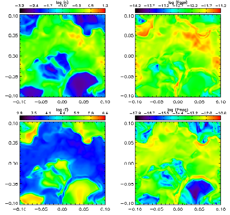
Figure 2: Two-dimensional slices through the three-dimensional model M8, parallel to the magnetic field at a time of 25 Myr, showing density (upper left), thermal pressure (upper right), temperature (lower left), and magnetic pressure (lower right). Color bars indicate the scale of each quantity, in units of cm^-3 for density $n$, K for temperature $T$, and dyne cm^-2 for both pressures. The axes are labeled in units of kpc.

We now examine the pressure distribution in our numerical simulations of a SN-driven, magnetized, interstellar medium. In Figure 2 we show density, pressure, and temperature, as well as magnetic pressure, on cuts through model M2 parallel to the magnetic field. (The perpendicular direction appears identical, because the flows are strongly super-Alfvénic, with rms Alfvén number exceeding four.) Examination of the pressure images immediately shows a broad variation in pressures among different regions in all the models, including in regions not closely associated with young SNRs. Regions with pressures markedly lower than ambient are apparent.

High temperature regions lie inside young SNRs, while low temperature regions have no uniform density and temperature correlation. The highest density regions have sizes of dozens of parsecs, and average densities approaching 100 cm^-3, typical of giant molecular clouds. This is consistent with the suggestion by Ballesteros-Paredes et al. (1999a) and Ballesteros-Paredes, Vázquez-Semadeni & Scalo (1999) that at least smaller molecular clouds are formed and destroyed by the action of the interstellar turbulence. Our models do not, however include self-gravity as do Li, Mac Low, & Klessen (2005) or Slyz et al. (2005), though neither includes magnetic fields (for recent reviews see Elmegreen 2002; Mac Low & Klessen 2004), isobaric thermal instabilities (Hennebelle & Pérault 1999, 2000; Burkert & Lin 2000; Vázquez-Semadeni, Gazol, & Scalo 2000; and Gazol et al. 2001), or thermal conduction (Koyama & Inutsuka 2004).

Even at SN rates four times those characteristic of the Milky Way, the hot medium in our models does not surround discrete clumps of cold and warm gas. Rather, discrete regions of hot gas are formed, occasionally intersect, and then seem to be dynamically mixed back into the warm gas that fills a substantial fraction of the space. This large-scale turbulent mixing appears to enhance the cooling rate, while sheets and filaments confined by nearby SNRs seem more effective at slowing down the expansion of SNRs than the isolated, discrete clumps of the same equivalent density suggested by MO77. These results are consistent with the results of Korpi et al. (1999), Avillez (2000), Avillez & Breitschwerdt (2004), and Slyz et al. (2005).

4.2 Thermodynamic Relations

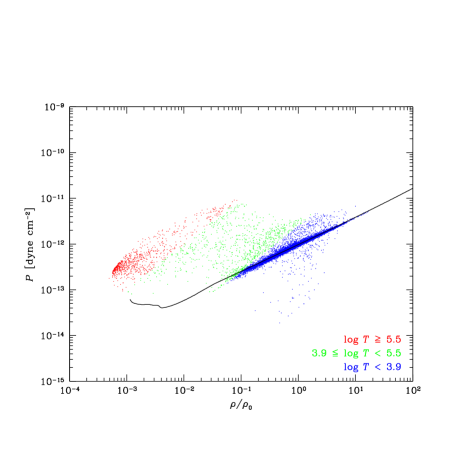
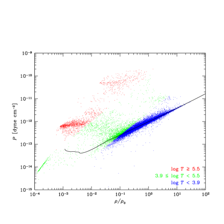
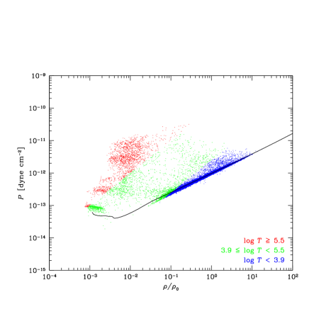
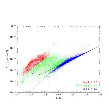
Figure 3: Scatter plot of pressure vs. density at $t=25$ Myr in models (a) M2, with low SN rate and high field, (b) M4, with high SN rate and field, (c) M6, with low SN rate and field, and (d) M8 with high SN rate and low field. We show a subset of $32^{3}$ points sampled at intervals of eight points in each direction, at 25 Myr for models M4 and M8, and 100 Myr for models M2 and M6. Cool gas with $\log T<3.9$ is shown in blue, warm gas with $3.9<\log T<5.5$ in green, and hot gas with $\log T>5.5$ in red. Temperature is given in K. The thermal equilibrium curve for the cooling and heating functions in this simulation is overlaid as a black line. Note that a wide variation of pressures is seen, and for each pressure, different densities occur.

The first theories of the multi-phase ISM, such as FGH, postulated an isobaric medium. Since then, multi-phase models have commonly been interpreted as being isobaric, although MO77 and Wolfire et al. (1995) actually assume only local pressure equilibrium, not global, and MO77 did consider the distribution of pressures, as described above in § 3.1. In multi-phase models, the heating and cooling rates of the gas have different dependences on the temperature and density, so that the balance between heating and cooling determines allowed temperatures and densities for any particular pressure. This balance can be shown graphically in a phase diagram, showing, for example, the allowed densities for any pressure (FGH; for a modern example, see Fig. 3(a) of Wolfire et al. 1995).

In Figure 3, the thermal-equilibrium curve for the heating and cooling mechanisms included in the models is shown as a black line. Only a single phase is predicted at high densities as our cooling curve did not include the physically-expected unstable region at temperatures of order $10^{3}$ K (Wolfire et al. 1995). Thus, if our model produced an isobaric medium, it would be expected to have a single low-temperature phase at uniform density given by the point at which the thermal-equilibrium curve crosses that pressure level. (Effectively, our cooling curve allows the hotter two of the three phases proposed by MO77.)

Figure 3 show the actual density and pressure of individual zones in the model. Many zones at temperatures in the range of $10^{3}$–$10^{4}$ K do lie on the thermal equilibrium curve, but scattered up and down it at many different pressures and densities, with no well-defined phase structure. Furthermore, a substantial fraction of the gas has not had time to reach thermal equilibrium at all after dynamical compression. It appears that pressures are determined dynamically, and the gas then tries to adjust its density and temperature to reach thermal equilibrium at that pressure. Most gas will land on the thermal equilibrium curve when dynamical times are long compared to heating and cooling times. This still leads to all points within the range of pressures available along the thermal equilibrium line being occupied, rather than the appearance of discrete phases. Unstable regions along the thermal equilibrium curve (Gazol et al. 2001) and off it will also be populated, as observed by Heiles (2001) for colder gas, but not as densely, as gas indeed attempts to heat or cool to a stable thermal equilibrium at its current pressure.

Comparison of the models shown in Figure 3(a)–(d) shows that the amount of gas that has not yet reached thermal equilibrium depends strongly on the SN rate, but that the basic conclusion that gas ends up in thermal equilibrium at a wide range of pressures does not. Magnetic fields play a secondary role, with higher field strength increasing the total pressure, but somewhat reducing the range of thermal pressures occupied. A stronger magnetic field does produce regions of low thermal pressure balanced by magnetic pressure that can be seen on and below the thermal equilibrium curve, as we further discuss below.

The range of pressures observed in our simulations is broader than the region shown by Wolfire et al. (1995) to be subject to thermal instability. Even models that included a proper cooling curve would produce some gas at pressures incapable of supporting a classical multi-phase structure. The mixture of different pressures will, however, produce gas at both high and low densities, as well as a smaller fraction of gas at intermediate densities that has not yet reached thermal equilibrium.

Under what conditions are the dynamical times indeed long compared to heating and cooling times? We can compare rough analytical estimates of each. The dynamical time is

$$t_{\rm dyn}=L/v_{\rm rms},$$ (8)

where $L$ is a characteristic length scale, while the cooling time

$$t_{\rm cool}=E/\dot{E}=kT/n\Lambda,$$ (9)

where $E$ is the thermal energy, and $\dot{E}=n^{2}\Lambda(T)$ is the cooling rate as a function of temperature $T$.

In model M2, for example, the rms velocity volume-averaged over gas of all temperatures is $v_{\rm rms}=55\mbox{ km s}^{-1}$. (This is the model with the smallest value of $v_{\rm rms}$.) If we take typical dynamical length scales of $L\sim 10$ pc, then $t_{\rm dyn}\simeq 0.2$ Myr. We tabulate $t_{\rm cool}$ from our cooling curve in Table 2, normalized to a density of $n=1$ cm^-3. (We note that model cooling times in gas at temperatures of $10^{3}\mbox{ K}\lesssim T\lesssim 10^{4}$ K are substantially less than physical values, as the MacDonald & Bailey cooling curve does not drop abruptly at $10^{4}$ K when Ly$\alpha$ cooling shuts off. However, the consequence of this is merely that our model overestimates the amount of gas that has reached thermal equilibrium: the scatter plot shown in Figure 3 should be even more uniformly filled.) At all temperatures $10^{3}$ K$<T<10^{7}$ K, we find that $t_{\rm cool}\ll t_{\rm dyn}$, especially at densities $n>1$ cm^-3. This agrees with our description of gas dynamics setting the local pressure and thermal equilibrium only then determining the density and temperature.

The separation between dynamical and thermal timescales also sheds light on the study by Vázquez-Semadeni et al. (2000) on the effects of turbulence on thermal instability. That study suggested that turbulence erases the effects of thermal instability on the interstellar medium. Our models show that turbulence probably didn’t erase the thermal instability entirely, but that the instability only acted locally, under the conditions set for it by the larger-scale turbulent flow. Also, thermal instability becomes less important in determining the overall distribution of pressures and temperatures when much of the gas has not even reached thermal equilibrium. More gas will lie in thermally stable regions than thermally unstable ones, but the wide range of available pressures and the lack of complete thermal equilibrium in many regions still results in a wide range of properties, despite the nominal action of the thermal instability.

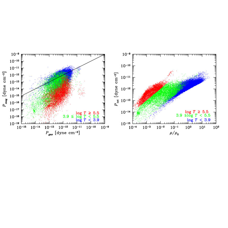
Figure 4: Scatter plot of (a) magnetic vs. thermal pressure and (b) total pressure vs. density at $t=25$ Myr in model M8. We again show a subset of $32^{3}$ points. In (a), many of the blue cold gas points have been covered by green warm and red hot gas points. The solid line shows equipartition between magnetic and thermal pressure. Much of the gas is far from equipartition in all temperature ranges.

The lower boundary of the heavily occupied region in the pressure-density plane appears to be determined by the polytropic behavior of the gas near this cutoff. Fitting to its slope yields values of the polytropic index $\gamma\sim$ 0.6–0.7. This can be understood as due to a cooling curve increasing as a power law (roughly $T^{2.9}$ can be fit) balanced by heating. Points lying below and to the right of this cutoff line at low pressures and high densities appear to be magnetically supported, dropping to very low thermal pressures at intermediate densities. This gas does not have low total pressure, only low thermal pressure, as shown in Figure 4(b).

In Figure 4(a), the relative strength of thermal and magnetic pressure is shown at one time for a magnetized simulation. Equipartition of thermal and magnetic pressure (plasma $\beta=P_{\rm gas}/P_{\rm mag}=1$) falls along the solid line. Gas at all temperatures often falls far from the equipartition line. In this model, both cold and warm gas have values of $\beta$ as low as 0.1, while at the high end, cold gas reaches $beta\sim 100$, and warm and hot gas have regions with $\beta$ as high as 10⁴. Magnetically supported regions occur in both cold and warm gas, as do thermally dominated regions. Hot gas can be seen, on the other hand, to be dominated by thermal pressure, with low magnetic pressures. In Figure 4(b), the total pressure is shown as a function of density for the same zones. Using total pressure, a clear cutoff at high densities and low pressures is now plain to see, showing that the previous scatter of points beyond it was due to small magnetically supported regions.

The wide range of magnetic pressures shown in Figure 4a calls into question the assumption of equipartition between magnetic and cosmic ray energy usually used to derive magnetic field strengths from radio synchrotron emission (Burn 1966, Sokoloff et al. 1998, Beck 2001). Large fluctuations in the magnetic field strength lead to overestimates of the strength of the regular magnetic field for given strength of polarized synchrotron emission. Beck (2001) estimates that fluctuations $\langle\delta B\rangle/\langle B\rangle\simeq 1$ lead to as much as a 40% overestimate in field strength or a factor of two overestimate in field energy. To measure the size of the fluctuations in our models, we take $\langle B\rangle=B_{\rm rms}$, and the fluctuating field $\langle\delta B\rangle$ to be the rms value of the field with the initial mean field $B_{0}$ subtracted off before taking the rms. The resulting values at the end of each of our runs, along with the ratio $\langle\delta B\rangle/\langle B\rangle$ are reported in Table 1. At lower field strengths, the fluctuations indeed approach order unity, and even with the high field strengths suggested by the synchrotron emission, $\langle\delta B\rangle/\langle B\rangle>0.5$. These results suggest that synchrotron emission observation may yield moderate to severe overestimates of the total field strength.

Finally, let us directly consider the distribution of pressures in gas at different temperatures. In Figure 5 we show scatter plots of thermal pressure against temperature. We note the concentration of points at temperatures below $10^{4}$ K, which once again reflects gas piling up in thermal equilibrium at a wide variety of pressures. The tilt to the left in Figure 5 occurs from the effective adiabatic index $\gamma<1$, with higher pressure gas typically having lower temperatures. Individual SNRs with roughly constant pressures are visible as stripes in the higher temperature region of the plot. As they cool, they also expand to lower pressures. Higher SN rate produces a broader distribution of temperatures in the low field case, where SN bubbles expand to fill more of the total volume.

4.3 Model Probability Distribution Functions

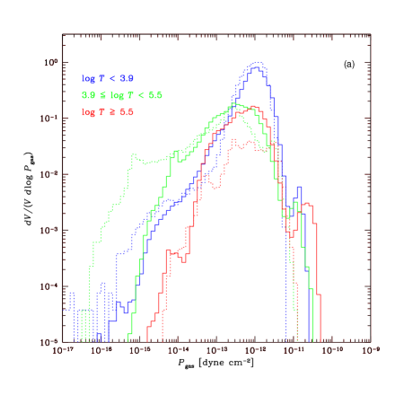
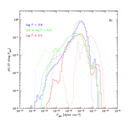
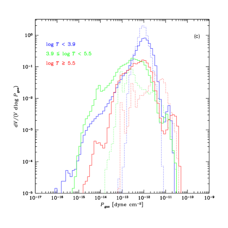
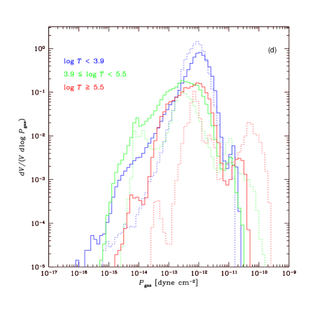
Figure 6: Volume-weighted PDFs of pressure for cool gas with $\log T<3.9$ (blue), warm gas with $3.9<\log T<5.5$ (green), and hot gas with $\log T>5.5$ (red) (a) at different resolutions of 1.56 pc (solid, model M8), and 3.13 pc (dotted, model M7), at 25 Myr, (b) at different times of 15 Myr (dashed) and 25 Myr (solid) in the 1.56 pc resolution model M8, (c) at different SN rates of Galactic (dotted, model M6) at 100 Myr, and four times Galactic (solid, model M8) at 25 Myr, and (d) at different initial magnetic field strengths of 2 $\mu$G (solid, model M8) and 5.8 $\mu$G (dotted, model M4) at 25 Myr.

We have shown that our models display a broad range of pressures. We can quantify this by examining the pressure PDFs, as shown in Figure 6. The first point to note, which we will return to below, is that all of our models show roughly log-normal pressure PDFs, unlike the power-law distributions predicted by the analytic theory derived by MO77 (see § 3.1). The observed distributions rather more resemble the pressure distributions suggested by PNJ97 and PV98 (see § 3.2). Not only is the total distribution broad, even at the Galactic SN rate (Fig. 6), but so is the distribution for different components of the interstellar medium individually. Furthermore, the typical or median pressure at the center of the PDF can vary with temperature, as demonstrated by the PDFs of gas at different temperature.

Our results do not appear to depend strongly on numerical resolution as demonstrated in Figure 6(a), although the details of the history of each SNR and the total amount of energy radiated away will certainly depend on the resolution, as well as on our neglect of the physics of the conductive interfaces between hot and warm gas. The pressure PDFs also appear to be stable over time, as shown by the comparison of multiple times in Figure 6(b), except for the hot gas, especially at the high-pressure end. Individual young SNRs produce discrete bumps that move left towards lower pressures as time passes, eventually merging with the overall distribution.

Figure 6(c) shows that increasing the SN rate produces a broader distribution of pressures, as generally predicted by both PNJ97 and PV98, and quantified below. Finally, Figure 6(d) shows that increasing the magnetic field strength reduces the amount of hot gas as SN remnants are better confined, and reduces the total amount of gas with low thermal pressure.

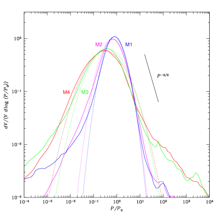
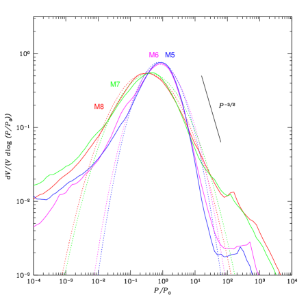
Figure 7: Volume-weighted PDFs (solid) and best fit Gaussians (dotted)of thermal pressure for magnetic field strengths of (a) $5.8\mu$G and (b) $2\mu$G for models with resolutions of 1.56 pc (red, purple), and 3.13 pc (green, blue), and SN rates of Galactic (blue, purple), averaged over 50 times from 75–100 Myr, and four times Galactic (red, green), averaged over 50 times from 18.75–25 Myr. Solid lines show the prediction of MO77 (taking $14/9\simeq 3/2$). Model names are noted on the figure.

Using the results for different SN rates illustrated in Figure 6(c), we can quantitatively test how well our results agree with the analytic descriptions of PV98 and PNJ97. We fit a simple log-Gaussian commensurate with the form of equation (7). These fits are shown in Figure 7 for all of our models. Although the Gaussians fit the peaks of our pressure PDFs reasonably well, exponential tails do appear in almost all cases.

We further include a line corresponding to the power law predicted by MO77, as given in our equation (2), noting that Figure 7 shows the log of the PDF, reducing the power law expected by a factor of unity from 23/9 to $14/9\simeq 3/2$. This prediction falls in between the values seen for the Galactic rate and the higher SN rate near the peak, and overpredicts the high-pressure tail at the Galactic rate, while underpredicting the tail at the higher rate. It does not appear to give a general description of our results. We further note that there is no hint of a gap in the differential pressure distribution corresponding to the lack of pressures just below the critical pressure for shell cooling in MO77 (see discussion above below eqn. (1).

We now compare the value of the dispersion of log pressure $\sigma$ that we find in our Gaussian fits to the predictions of PNJ97 and PV98 given in § 3.2. As an approximation to $x_{0}$, the log of the average pressure, we take the peaks of the PDFs (the modes). We then use the rms velocities of each model, to predict $\sigma_{x}$. In Table 1 we give these values, and in Figure 8 we compare the fits to the widths predicted by the rms Mach number for both descriptions. Our results agree reasonably well with the prediction for PNJ97, and disagree strongly with that for PV98.

Ostriker et al. (2001) and Li, Klessen, & Mac Low (2003) have noted the failure of PV98 to predict the PDFs for three-dimensional, uniformly-driven turbulence with both isothermal and non-isothermal equation of state, suggesting that the difference in results between PNJ97 and PV98 is due to the use of one-dimensional runs in PV98. The generally good agreement we find here with PNJ97 is perhaps somewhat surprising, given that their result was derived for uniformly-driven, isothermal, turbulence, while we include a non-isothermal equation of state, supernova explosions, and a magnetic field. All of these effects appear to play only a secondary role, however. Li et al. (2005) show that the assumption of an isothermal equation of state appears to be sufficient to explain the gross star-forming properties of galaxies, so perhaps our result is not entirely far-fetched.

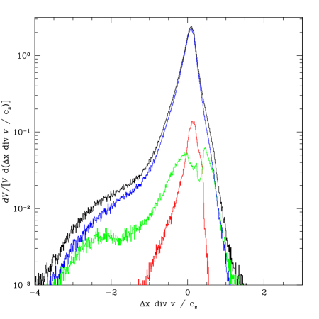
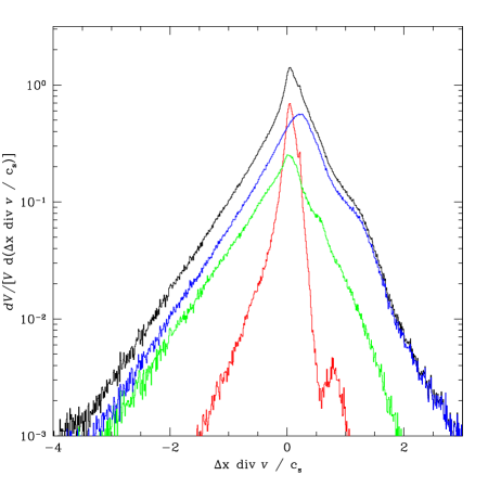
Figure 9: Volume-weighted PDF of the divergence of velocity normalized by sound speed $\nabla\cdot\vec{v}/c_{s}$ for low field models with supernova rates of (a) Galactic (model M6) and (b) four times Galactic (model M8). Negative values greater trace compressions and shocks, while positive values trace rarefaction waves and expanding flows. Note the general symmetry between positive and negative values at the peaks of the PDFs, supporting the theory that the density and pressure distribution is determined by a random series of shocks and rarefactions.

The Gaussian form of the PDF used by both PNJ97 and PV98 was inspired by the theory of Vázquez-Semadeni (1994) who argued that the density fluctuation spectrum in a strongly supersonic flow is built up by a random series of compressions and rarefactions. We can directly trace compressions and rarefactions by examining the distribution of $\nabla\cdot\vec{v}$ in our models (Fig. 9). This distribution is generally symmetric around the peak at zero, with compressions on the negative side and rarefactions on the positive side appearing nearly equally common. This supports the idea that the density and pressure fluctuation spectra are generated by repeated compressions and rarefactions occurring with equal probability.

The question of how mass is distributed among regions of different pressure becomes important when considering questions such as the potential ram-pressure confinement of molecular clouds. The mass distribution might be expected to markedly diverge from the volume distribution given by the PDFs shown previously, as most of the hot gas resides at very low densities. In Figure 10 we show mass-weighted distribution functions from each high-resolution model. The cold gas dominates the mass-weighted PDF, but it is found at the same wide range of pressures, with roughly the same peak pressure, as was suggested by the volume-weighted PDFs shown earlier. In particular, a substantial fraction of the mass in the cold gas lies at pressures five to ten times higher than the average pressure, even in the absence of self-gravity.

5 Comparison to Observations

5.1 Ionized and Atomic Gas

Evidence for a broad distribution of interstellar pressures had already been noted as early as the work on excited levels of Ci by Jenkins & Shaya (1979) and Jenkins et al. (1983). The point was sharpened with the direct comparison of nearby pressures by Bowyer et al. (1995), who compared the pressure of the interstellar medium impinging on the heliosphere with the pressure of the interstellar medium averaged over a 40 pc line of sight as measured with the Extreme Ultraviolet Explorer. Jenkins & Tripp (2001) have used the STIS to extend the work on Ci with better resolved data, concluding that the pressure varies by over an order of magnitude both above and below the average value in a small fraction of the gas. Our models naturally explain these variations in the context of a SN-driven interstellar medium.

Jenkins et al. (1983) compared their results to the analytic theory of MO77, described above in § 3. They found a substantially greater column density of low-pressure material than that predicted, and rather less high-pressure material. As the analytic theory could not predict pressures much less than average, while our models show a broad range of rarefaction waves producing a log-normal pressure distribution around the mean, the low-pressure results appear consistent. Jenkins et al. were observing emission from excited states of Ci in low-temperature gas. We find that much or most of the high-pressure gas resides in the hot medium, so, although we do predict a greater total volume of high-pressure gas than was predicted by MO77, we expect that most of it would have been ionized, and therefore not observable by Jenkins et al. (1983), explaining their low column densities of high-pressure material.

Bowyer et al. (1995) and Berghöfer et al. (1998) derived a lower limit to average pressure derived from extreme ultraviolet emission along lines of sight to H i clouds in the Local Bubble. The cloud distances were determined using photometry of stars superposed on the cloud boundaries. They found a pressure of $P/k>$13,500–16,500 K cm^-3 for the hot medium, with the error depending mostly on the choice of plasma code used to derive the emission. They compared this to the value for the pressure in the Local Cloud of 700–760 K cm^-3 derived by Frisch (1994) from scattering of solar He i 584Åradiation from helium flowing in from the cloud through the heliosphere. McKee (1996) argues that a more careful treatment of the unknown ionization fraction could lead to a local pressure a factor of three higher, reducing, but not eliminating, the discrepancy. We find greater than order of magnitude variations in our models, with pressures reaching values as low as a few hundred K cm^-3 in isolated regions in both sets of models. Interestingly, the lowest pressures in our models occur at moderately low densities of order 0.1 cm^-3, while the density derived for the Local Cloud by, for example, Quemerais et al. (1994) is 0.14 cm^-3.

An example of a region with high and low pressure regions intertwined in the manner suggested by the EUV observations is the superbubble seen in the corners of Figure 2, particularly the part in the upper left corner (note that we are using periodic boundary conditions). In this region, even local pressure equilibrium is lacking on scales of tens of parsecs, in contrast to all multi-phase models. Similar regions form regularly over time.

Jenkins & Tripp (2001) found that their results implied an effective polytropic index in the cold gas of $\gamma>0.9$, somewhat higher than the $\gamma=0.72$ derived by Wolfire et al. (1995) for this gas. The suggestion advanced to explain this is that the regions being compressed may be smaller than the cooling length scale, and so may begin to behave adiabatically. An alternative explanation may be drawn from the broad range of pressures at which gas cools in our model: the (relatively sudden) pressurization may happen prior to cooling, rather than to already cooled gas, as required by the derivation of $\gamma$ by Jenkins & Tripp.

5.2 Molecular Gas

Molecular clouds are observed to have broad linewidths suggesting that they are subject to pressures as high as $10^{5}$ K cm^-3. Larson (1981) was one of the first to suggest that the effective pressure was due to the self-gravity of the cloud. Since then, several authors have found that most of the individual clumps in molecular clouds are not in hydrostatic balance between turbulent pressure and self-gravity, but rather are confined by an external pressure (Carr 1987; Loren 1989; Bertoldi & McKee 1992). The explanation offered for this by Bertoldi & McKee (1992) was that the entire cloud was still subject to self-gravity, even though individual clumps were not, and so the effects of self-gravity on large scales produced pressures that confined the clumps.

In our models, we find pressures in high-density regions of order $10^{5}$ K cm^-3 in the absence of self-gravity, as shown in Figure 3. These pressures are sufficient to confine observed clumps without invoking self-gravity, suggesting that observed molecular clouds may be primarily pressurized by the ram pressure of the turbulent flows in which they are embedded rather than being self-gravitating objects. Simulated observations of turbulent flows suggest that mass-linewidth relations thought to indicate that they are in virial equilibrium may actually be due to a combination of the properties of the turbulence itself in the case of the size-linewidth relation, and the properties of the observations in the case of the size-mass relation (Vázquez-Semadeni, Ballesteros-Paredes, & Rodriguez 1997; Ballesteros-Paredes, & Mac Low 2002).

Ram pressure is a double-edged sword, however, that can destroy clouds as easily as creating them. This is consistent with the suggestion that they are transient objects with lifetimes of under $10^{7}$ yr first made by Larson (1981), and emphasized by Ballesteros-Paredes, et al. (1999a), Elmegreen (2000, 2002), and Hartmann et al. (2001). Relying on ram pressures rather than self-gravity to confine observed clumps in molecular clouds would also be consistent with the results of simulations of hydrodynamical and MHD driven, self-gravitating, isothermal turbulence that showed self-gravity only acting on small scales, with turbulent flows dominating the large scales (Klessen et al. 1999; Heitsch et al. 2001). The same flows that confine and destroy the clumps also drive the turbulence observed within them, as the background flow stretches, twists, forms, and destroys dense regions contained within it.

Our prescription of isochoric nonequilibrium cooling for $10^{4}\mbox{ K}<T<10^{6}$ K, and more especially the absence of the physically expected region of thermal instability at $T<10^{4}$ K prevents us from having any degree of confidence in the exact amounts of cold gas produced at any given pressure. However, our qualitative results appear quite robust, so we expect future work to refine the details rather than substantially change the picture of molecular clouds forming in transient, high-pressure, high-density regions produced by a supersonic, turbulent flow.

6 Discussion and Summary

We have examined the distribution of pressures predicted from three-dimensional simulations of a SN-driven, magnetized ISM, neglecting vertical stratification and self-gravity, but including a distributed heating function. In all the simulations we have run, we find pressures distributed over rather more than an order of magnitude around the mean. The pressure PDF can be fit well with a log-normal having width given by the analytic description of PNJ97 based on three-dimensional simulations of isothermal turbulence, and disagreeing with the one-dimensional results of PV98. The log-normal distribution is predicted by the theory of Vázquez-Semadeni (1994) that density fluctuations in a supersonic turbulent flow result from a sequence of random compressions and rarefactions. We find that compressions and rarefactions are indeed symmetrically distributed, lending further support to this idea. The log normal form differs from the power-law distribution predicted by MO77. The only isobaric regions found in our models are the interiors of young SNRs; these are also the only laminar flow regions in an otherwise turbulent environment.

Most of the mass is in the turbulent gas, however, as is most of the volume, even in models driven with four times the Galactic supernova rate. This result is consistent with the results of Korpi et al. (1999), Avillez (2000), and Avillez & Breitschwerdt (2004). The last group performed a resolution study to establish that numerical diffusion was not causing hot gas to cool unphysically. We will study the filling factors of our models in more detail in future work.

We find a broad range of pressures, and a substantial fraction of associated densities, far from the thermal equilibrium values. This limits the predictive usefulness of phase diagrams based on thermal equilibrium, although thermal equilibrium at the local pressure is still the mildly favored state. Gas pressures appear to be determined dynamically. Each individual parcel of gas seeks local thermal equilibrium at the pressure imposed on it by the turbulent flow. As suggested by previous authors, the phase diagram is only locally valid. Isobaric thermal instability in such an environment will lead to regions of the phase diagram being mildly disfavored, but no more. Vázquez-Semadeni et al. (2000) and Gazol et al. (2001) used two-dimensional simulations with more physically-motivated cooling curves at lower temperatures to conclude that the effects of the thermal instability will be barely visible in the overall probability distribution functions (but note that these simulations did not resolve cooling regions well, so the results should be taken with caution).

Our results appear consistent with observations that have repeatedly shown the ISM not to be isobaric, including those by Jenkins & Shaya (1979), Jenkins, Jura & Loewenstein (1983), Bowyer et al. (1995), Berghöfer et al. (1998), and Jenkins & Tripp (2001). Although heating and cooling rates remain important for determining the local density and temperature, they do not produce a global multi-phase medium with well-separated regions of different temperature gas because of the wide range of pressures present and the dynamical processing of the gas. Rather, a more continuous distribution of temperatures and densities is always present.

The inference that most molecular clouds must be gravitationally bound because of their high observed confinement pressures are called into question by our results. Regions with densities approaching the overall densities of GMCs, and pressures an order of magnitude above the average interstellar pressure appear in our simulations even in the absence of self-gravity. This supports suggestions that star-forming molecular clouds may be transient, turbulently-driven, objects (Ballesteros-Paredes et al. 1999ab, Elmegreen 2000, 2002, Hartmann et al. 2001). Objects that do gravitationally collapse from large scales as described, for example by Kim & Ostriker (2001), Elmegreen (2002), or Li et al. (2005) will also form molecular gas, but will quickly form starburst knots in a burst of violent, unimpeded star formation.

Magnetic pressures are also broadly distributed, and do not correlate well with thermal pressures. The ratio of thermal to magnetic pressure $\beta$ takes on values ranging from 0.1 to as much as 100 in gas with temperatures under $10^{4}$ K, and much higher values in hot gas. The ratio of fluctuating to mean field in our models $\langle\delta B\rangle/\langle B\rangle=0.5$–1, high enough to suggest that field strengths derived from observations of polarized synchrotron emission may be overestimated (Beck 2001).

Figures

Figure 1: Convergence study of shell radius for a single SN remnant in a cold, unmagnetized medium. The analytic expression from Cioffi et al. (1988) (line) is compared to simulations in a 200 pc box using grids of $64^{3}$ (circles), $128^{3}$ (triangles), and $256^{3}$ (squares) zones. Good agreement is obtained at $128^{3}$ resolution. Stair steps in the numerical curves come from only being able to measure the size of the shell to the nearest integral zone.

Figure 5: Scatter plot of pressure vs. temperature at $t=25$ Myr in models (a) M2, with low SN rate and high field, (b) M4, with high SN rate and field, (c) M6, with low SN rate and field, and (d) M8 with high SN rate and low field. We again show a subset of $32^{3}$ points, and give temperature in K.

Figure 8: Comparison of predictions of PDF width as a function of volume-weighted rms Mach numbers from analytic descriptions of supersonic, uniformly-driven, hydrodynamic, isothermal turbulence by PNJ97 (solid) and PV98 (dotted) to our low-resolution (crosses) and high-resolution (triangles) results. The description of PNJ97 agrees far better with our results. Low-resolution models have widths very similar to their corresponding high-resolution models, although their Mach numbers differ more significantly in the high SN rate cases.

Figure 10: Mass-weighted PDF of pressure in low field models with SN rates of Galactic (dotted, model M6) at a time of 100 Myr, and four times Galactic (solid, model M8) at 25 Myr, for all the gas (upper left), cool gas with $\log T<3.9$ (upper right), warm gas with $3.9<\log T<5.5$ (lower left), and hot gas with $\log T>5.5$ (lower right). Most of the mass is found in cold gas, with a broad distribution around the peak pressure.

Table 1: Model Properties.

model	$\tau_{\rm SN}$	$\Delta x_{\rm min}$	$B_{0}$	$\langle B\rangle$	$\langle\delta B\rangle$	$\langle\delta B\rangle$	$M_{\rm rms}$	$\sigma$
		(pc)	($\mu$G)	($\mu$G)	($\mu$G)	$\langle B\rangle$
M1	1	3.13	5.8	6.258	3.063	0.489	0.947	0.3666
M2	1	1.56	5.8	6.443	3.470	0.539	1.039	0.4100
M3	4	3.13	5.8	6.685	4.430	0.663	1.442	0.6266
M4	4	1.56	5.8	7.049	4.778	0.678	1.545	0.6859
M5	1	3.13	2.0	2.436	1.854	0.761	0.947	0.5222
M6	1	1.56	2.0	2.589	2.071	0.800	0.941	0.5575
M7	4	3.13	2.0	2.587	2.610	1.009	1.353	0.7423
M8	4	1.56	2.0	3.071	3.067	0.999	1.580	0.7378

Table 2: Cooling Times

$\log_{10}T$	$t_{\rm cool}(n/1\mbox{ cm}^{-3})^{-2}$
(K)	(yr)
3	1.7(5)
4	6.0(3)
5	1.6(3)
6	4.4(4)
7	1.2(6)

References

- (1) Avillez, M. A. 2000, MNRAS, 315, 479
- (2) Avillez, M. A., & Breitschwerdt, D. 2004, A&A, 425, 899
- (3) Ballesteros-Paredes, J., Hartmann, L., & Vázquez-Semadeni, E. 1999a, ApJ, 527, 285
- (4) Ballesteros-Paredes, J., & Mac Low, M.-M. 2002, 570, 734
- (5) Ballesteros-Paredes, J., Vázquez-Semadeni, E., & Scalo, J. 1999b, ApJ, 515, 286
- (6) Balsara, D. S. 1998a, ApJS, 116, 119
- (7) Balsara, D. S. 1998b, ApJS, 116, 133
- (8) Balsara, D. S. 2000, Rev. Mex. Astron. Astrof. Ser. Conf., 9, 92
- (9) Balsara, D. S. 2001, J. Comput. Phys., 174, 614
- (10) Balsara, D. S. 2004, ApJS, 151, 149
- (11) Balsara, D. S., & Kim, J. 2004, ApJ, 602, 1079
- (12) Balsara, D. S., Kim, J., & Mac Low, M.-M. 2001, J. Kor. Astron. Soc., 34, 333
- (13) Balsara, D. S., Kim, J., Mac Low, M.-M., & Mathews, G. 2004, ApJ, in press
- (14) Balsara, D. S., & Norton, C. 2001, Parallel Comput., 27, 37
- (15) Balsara, D. S., & Spicer, D. S. 1999, J. Comput. Phys., 148, 133
- (16) Beck, R. 2001, Sp. Sci. Rev., 99, 243
- (17) Bell, J., Berger, M. Saltzman, J., & Welcome, M. 1994, SIAM J. Sci. Stat. Comput., 15, 127
- (18) Berger, M. J., & Colella, P. 1989, J. Comput. Phys., 82, 64
- (19) Berghöfer, T. W., Bowyer, S., Lieu, R., & Knude, J. 1998, ApJ, 500, 838
- (20) Bertoldi, F., & McKee, C. F. 1992, ApJ, 395, 140
- (21) Bowyer, S., Lieu, R., Sidher, S. D., Lampton, M., & Knude, J. 1995, Nature, 375, 212
- (22) Blitz, L., Shu, F. H. 1980, ApJ, 238, 148
- (23) Burkert, A., & Lin, D. N. C. 2000, ApJ, 537, 270
- (24) Burn, B. J. 1966, MNRAS, 133, 67
- (25) Cappellaro, E., Turatto, M., Tsvetkov, D. Y., Bartunov, O. S., Pollas, C., Evans, R., & Hamuy, M. 1997, A&A, 322, 431
- (26) Carr, J. S. 1987, ApJ, 323, 170
- (27) Cioffi, D. F., McKee, C. F., & Bertschinger, E. 1988, ApJ, 334, 252
- (28) Colella, P., & Woodward, P. 1984, J. Comput. Phys., 54, 174
- (29) Cox, D. P., & Smith, B. W. 1974, ApJ, 189, L105
- (30) Dalgarno, A., & McCray, R. A. 1972, ARA&A, 10, 375
- (31) Dickey, J. M., & Lockman, F. J. 1990, ARA&A, 28, 215
- (32) Elmegreen, B. G. 2000, ApJ, 530, 277
- (33) Elmegreen, B. G. 2002, ApJ, 577, 206
- (34) Ferrière, K. 1998, ApJ, 503, 700
- (35) Field, G. B., Goldsmith, D. W., & Habing, H. J. 1969, ApJ, 155, L149 (FGH)
- (36) Frisch, P. 1994, Science, 265, 1423
- (37) Fukui, Y., et al. 1999, PASJ, 51, 745
- (38) Gazol, A., Vázquez-Semadeni, E., Sánchez-Salcedo, F. J., & Scalo, J. 2001, ApJ(Letters), 557, L121
- (39) Hartmann, L., Ballesteros-Paredes, J., & Bergin, E. A. 2001, ApJ, 562, 852
- (40) Heiles, C. 2001, ApJ, 551, L105
- (41) Heitsch, F., Mac Low, M.-M., & Klessen, R. S. 2001, ApJ, 547, 280
- (42) Hennebelle, P., & Pérault, M. 1999, A&A, 351, 309
- (43) Hennebelle, P., & Pérault, M. 2000, A&A, 359, 1124
- (44) Jenkins, E. B., Jura, M., & Loewenstein, M. 1983, ApJ, 270, 88
- (45) Jenkins, E. B., & Shaya, E. J. 1979, ApJ, 231, 55
- (46) Jenkins, E. B., & Tripp, T. M. 2001, ApJS, 137, 297
- (47) Kim, W.-T. & Ostriker, E. C. 2001, ApJ, 559, 70
- (48) Klessen, R.S., Heitsch, F., Mac Low, M.-M. 1999, ApJ, 535, 887
- (49) Korpi, M. J., Brandenburg, A., Shukurov, A., Tuominen, I., Nordlund, Å. 1999, ApJ, 514, L99
- (50) Koyama, H., & Inutsuka, S.-I. 2004, ApJ, 602, L25
- (51) Larson, R. B. 1981, MNRAS, 194, 809
- (52) Li, Y., Klessen, R. S., Mac Low, M.-M. 2003, ApJ, 592, 975
- (53) Li, Y., Mac Low, M.-M., & Klessen, R. S. 2005, ApJ, in press (astro-ph/0407247)
- (54) Lockman, F. J., Hobbs, L. M., Shull, J. M. 1986, ApJ, 301, 380
- (55) Loren, R. B. 1989, ApJ, 338, 925
- (56) Mac Low, M.-M. 2000, in Stars, Gas, and Dust in Galaxies: Exploring the Links, eds. D. Alloin, K. Olsen, & G. Galaz (San Francisco: ASP), 55
- (57) Mac Low, M.-M., Balsara, D. S., Avillez, M. A., & Kim, J. 2001, unpub. (astro-ph/0106509)
- (58) MacDonald, J., & Bailey, M. E. 1981, MNRAS, 197, 995
- (59) McCray, R., & Kafatos, M. 1987, ApJ, 317, 190
- (60) McKee, C. F. 1996, in The Interplay Between Massive Star Formation, the ISM, and Galaxy Evolution, eds. D. Kunth, B. Guiderdoni, M. Heydari-Malayeri, & T. X. Thuan (Ed. Frontieres: Gif-sur-Yvette, France), 223
- (61) McKee, C. F., & Ostriker, J. P. 1977, ApJ, 218, 148 (MO77)
- (62) Nordlund, Å, & Padoan, P. 1999, in Interstellar Turbulence, eds. J. Franco, & A. Carramiñana (Cambridge U. Press, Cambridge, UK), 218
- (63) Ostriker, E. C., Stone, J. M., & Gammie, C. F. 2001, ApJ, 546, 980.
- (64) Padoan, P. Nordlund, Å, & Jones, B. J. T. 1997, MNRAS, 288, 145 (PNJ97)
- (65) Passot, T., & Vázquez-Semadeni, E. 1998, Phys. Rev. E, 58, 4501 (PV98)
- (66) Quémerais, E., Bertaux, J.-L., Sandel, B. R., & Lallement, R. 1994, A&A, 290, 941
- (67) Rand, R. J., & Kulkarni, S. R. 1989, ApJ, 343, 760
- (68) Raymond, J. C., Cox, D. P., & Smith, B. W. 1976, ApJ, 204, 290
- (69) Reynolds, R. J. 1987, ApJ, 323, 118
- (70) Roe, P. L., & Balsara, D. S. 1996, SIAM J. Appl. Math., 56, 57
- (71) Rosen, A. & Bregman, J. N. 1995, ApJ, 440, 634
- (72) Shapiro, P. R., & Moore, R. T. 1976, ApJ, 207, 460
- (73) Slavin, J. D., & Cox, D. P. 1993, ApJ, 417, 187
- (74) Slyz, A. D., Devriendt, J. E. G., Bryan, G., & Silk, J. 2005, MNRAS, 356, 737
- (75) Sokoloff, D. D., Bykov, A. A., Shukurov, A., Berkhuijsen, E. M., Beck, R., & Poezd, A. D. 1998, MNRAS, 299, 189.
- (76) Spitzer, L. 1956, ApJ, 124, 20
- (77) Strange W. G., 1968, SIAM J. Numer. Anal., 5, 506
- (78) Tammann, G. A., Löffler, W., & Schröder, A. 1994, ApJS, 92, 487
- (79) Vázquez-Semadeni, E. 1994, ApJ, 423, 681
- (80) Vázquez-Semadeni, E., Ballesteros-Paredes, J., & Rodriguez, L. F. 1997, ApJ, 474, 292
- (81) Vázquez-Semadeni, E., Gazol, A., & Scalo, J. 2000, ApJ, 540, 271
- (82) Vázquez-Semadeni, E., Passot, T., Pouquet, A. 1995, ApJ, 473, 881
- (83) Wolfire, M. G., McKee, C. F., Hollenbach, D., & Tielens, A. G. G. M., & Bakes, E. L. O. 1995, ApJ, 443, 152