The DEEP2 Galaxy Redshift Survey: First results on galaxy groups

Abstract

We use the first 25% of the DEEP2 Galaxy Redshift Survey spectroscopic data to identify groups and clusters of galaxies in redshift space. The data set contains 8370 galaxies with confirmed redshifts in the range $0.7\leq z\leq 1.4$, over one square degree on the sky. Groups are identified using an algorithm (the Voronoi-Delaunay Method) that has been shown to accurately reproduce the statistics of groups in simulated DEEP2-like samples. We optimize this algorithm for the DEEP2 survey by applying it to realistic mock galaxy catalogs and assessing the results using a stringent set of criteria for measuring group-finding success, which we develop and describe in detail here. We find in particular that the group-finder can successfully identify $\sim 78\%$ of real groups and that $\sim 79\%$ of the galaxies that are true members of groups can be identified as such. Conversely, we estimate that $\sim 55\%$ of the groups we find can be definitively identified with real groups and that $\sim 46\%$ of the galaxies we place into groups are interloper field galaxies. Most importantly, we find that it is possible to measure the distribution of groups in redshift and velocity dispersion, $n(\sigma,z)$, to an accuracy limited by cosmic variance, for dispersions greater than $350\mathrm{\;km\;s^{-1}}$. We anticipate that such measurements will allow strong constraints to be placed on the equation of state of the dark energy in the future. Finally, we present the first DEEP2 group catalog, which assigns 32% of the galaxies to 899 distinct groups with two or more members, 153 of which have velocity dispersions above $350\mathrm{\;km\;s^{-1}}$. We provide locations, redshifts and properties for this high-dispersion subsample. This catalog represents the largest sample to date of spectroscopically detected groups at $z\sim 1$.

1. Introduction

Groups and clusters of galaxies are the most massive dynamically relaxed objects in the universe; as such, they have long been the subject of intense and fruitful study. More than seventy years ago observations of the Coma cluster gave the first evidence for the existence of dark matter (Zwicky 1933). More recently, studies of gravitational lensing by clusters have yielded intriguing new information about the profiles of dark matter halos (Sand et al. 2004). Identifying and studying galaxies in groups and clusters is essential to understanding the effects of local environment on galaxy formation and evolution (for a review see Bower & Balogh 2004). X-ray measurements of the gas mass fraction in clusters have been used to constrain the mass density parameter $\Omega_{M}$ and more recently the equation of state of the dark energy, $w$ (e.g., Allen et al. 2004, and references therein). Finally, if we can accurately measure the abundance of groups and its evolution with redshift, we can constrain the growth of large-scale structure, thereby placing significant further constraints on cosmological parameters (Lilje 1992; Eke et al. 1996; Borgani et al. 1999; Haiman et al. 2001; Holder et al. 2001; Newman et al. 2002).

A wide array of methods has been used to identify groups and clusters at moderate redshifts: X-ray emission from hot intracluster gas (reviewed by Rosati, Borgani & Norman 2002), cosmic shear due to weak gravitational lensing (reviewed by Refregier 2003), searches in optical photometric data (e.g., Gonzalez et al. 2001; Yee & Gladders 2002), the Sunyaev-Zel’dovich (SZ) effect in the Cosmic Microwave Background (e.g., LaRoque et al. 2003), and direct reconstruction of three-dimensional objects in galaxy redshift surveys (e.g., Eke et al. 2004). To study the evolution of the group abundance it is necessary to extend observations to more distant objects. However, most of the methods used for local studies have only limited effectiveness at high redshift. The apparent surface brightness of X-ray clusters dims as $(1+z)^{-4}$, making only the richest clusters visible at high redshift. The cross-section for gravitational lensing falls rapidly at high redshifts, making weak-lensing detection of distant clusters difficult for all but the most massive objects. In photometric surveys, the increased depth necessary for high-redshift studies increases the overall number density of objects, thereby increasing the problems of foreground and background contamination and projection effects (though photometric techniques for estimating redshifts can mitigate these difficulties). The SZ effect is very promising, since it is entirely independent of redshift, but it also suffers from confusion limits and projection effects, and in any case a large survey of SZ clusters is yet to be undertaken. For the time being, then, one of the few methods that can be applied to large numbers of groups and clusters on similar mass scales at $z\sim 0$ and $z\sim 1$ is the direct detection of these structures in the redshift-space distribution of galaxies.

The first sizeable sample of groups detected in redshift space was presented by Geller & Huchra (1982), who found 176 groups of three or more galaxies in the CfA galaxy redshift survey at redshifts $z\lesssim 0.03$. Recently, Eke et al. (2004) identified groups within the final data release of the Two-degree Field Galaxy Redshift Survey (2dFGRS). Their catalog extends to $z\approx 0.25$ and constitutes the largest currently available catalog of galaxy groups, containing $\sim 3\times 10^{4}$ groups with two or more members. A comprehensive listing of previous studies of local optically selected group samples is also given by these authors. Work is currently underway to detect groups of galaxies in the spectroscopic data of the Sloan Digital Sky Survey (Nichol 2004). Studies of groups detected in redshift space were extended to intermediate redshifts by Carlberg et al. (2001), who found more than 200 groups in the CNOC2 redshift survey, with redshifts in the range $0.1\leq z\leq 0.55$. Additionally, Cohen et al. (2000) studied a sample of 23 density peaks in redshift space, over the redshift range $0\leq z\leq 1.25$. Until now, however, no spectroscopic sample has existed with sufficient size, sampling density and redshift accuracy to extend redshift-space studies of large numbers of groups to redshifts $z\gtrsim 0.5$.

The DEEP2 Galaxy Redshift survey (Davis et al. 2003; Faber et al. in prep.) is the first large spectroscopic galaxy catalog at high redshift, with observations planned for $\sim 5\times 10^{4}$ galaxies, most of which will fall in the range $0.7\leq z\leq 1.4$. The survey is thus a unique dataset for studying high-redshift galaxy groups. With such a broad range in redshift, we expect to observe evolution in the properties of galaxies, groups, and clusters within the DEEP2 sample itself; also, by comparing to local samples from 2dFGRS and the Sloan Digital Sky Survey (SDSS), we expect to observe evolution between $z\sim 1$ and the present epoch. DEEP2 is especially well-suited to studies of groups, since its high redshift accuracy allows detailed studies of their internal kinematics. Repeated observations of some DEEP2 galaxies indicate a velocity accuracy $\delta v\approx 25\mathrm{\;km\;s^{-1}}$, considerably better than the 2dFGRS value $\delta v\approx 85\mathrm{\;km\;s^{-1}}$ (Colless et al. 2001) and similar to the $\delta v\approx 30\mathrm{\;km\;s^{-1}}$ attained in the SDSS (Stoughton et al. 2002). In particular, it will be possible to estimate the masses of DEEP2 groups from their velocity dispersions. We anticipate that, by measuring the evolution of the group velocity function with redshift, it will be possible to constrain cosmological parameters such as the dark energy density parameter $\Omega_{\Lambda}$ and equation of state parameter $w$, as outlined in Newman et al. (2002). Before carrying out such studies, however, it will be essential to develop robust methods for detecting groups and clusters within DEEP2.

Identifying groups and clusters in redshift space is well known to be a difficult task. Most notably, clustering information is smeared out by redshift space distortions like the so-called fingers-of-God effect, in which galaxies in groups and clusters appear highly elongated along the line of sight because of intracluster peculiar motions. This intermingles group members with other nearby galaxies and causes neighboring groups to overlap in redshift space. A group-finding algorithm that attempts to find all group members will thus necessarily be contaminated by interloper field galaxies and will necessarily merge some distinct groups together into spurious larger structures. Conversely, a group finder that aims to minimize contamination and over-merging will fragment some larger clusters into smaller groups. This trade-off in group-finding errors is well known (e.g., Nolthenius & White 1987) and fundamentally unavoidable. It will therefore be essential, before we begin any program of group finding, to construct a suitable definition of group-finding success, identifying in advance which errors we seek to minimize and what sort of errors we are willing to tolerate. Ultimately, the chosen definition of success will depend on the intended scientific purpose of the group catalog. A major portion of this paper will be devoted to defining appropriate measures of group-finding success for the DEEP2 survey and optimizing our methods using these criteria.

This paper is organized as follows. In Section 2 we introduce the DEEP2 sample and discuss the unique opportunities and difficulties it presents for group finding. In the same section we describe the DEEP2 mock galaxy catalogs, which we will use to calibrate our group-finding methods. Then, in Section 3, we describe our criteria for group-finding success. In Section 4, we give an overview of various group-finding methods that have been used in the literature, and we describe the Voronoi-Delaunay Method (VDM) of  Marinoni et al. (2002), which we will use in this study. We then proceed to optimize this method for the DEEP2 sample. Finally, in Section 5, we apply the VDM algorithm to the current DEEP2 observations and present the first DEEP2 group catalog.

2. Group finding in the DEEP2 survey

2.1. The DEEP2 sample

As mentioned, the DEEP2 Galaxy Redshift Survey is the first large (tens of thousands of galaxies) spectroscopic survey of galaxies at high redshifts, $z\sim 1$. The goal of the survey is to obtain spectra of $\sim 5\times 10^{4}$ objects over $3.5\;\mathrm{deg}^{2}$ on the sky to a limiting magnitude of $R_{AB}=24.1$ using the DEIMOS spectrograph on the Keck II telescope. Typical redshifts in the survey fall in the range $0.7\leq z\leq 1.4$. Details of the survey will be described comprehensively in an upcoming paper by Faber et al. (in prep.); we summarize the salient information for this study here.

The survey consists of four fields on the sky, chosen to lie in zones of low Galactic dust extinction. Three-band ($BRI$) photometry has been obtained for each of these fields using the CFH12K camera on the Canada-France-Hawaii Telescope (CFHT), as described by Coil et al. (2004b). In three of the fields, which each consist of three contiguous CFHT pointings covering a strip of 120 arcmin by 30 arcmin, galaxies are selected for spectroscopy if they pass a simple cut in color-color space. This cut reduces the fraction of galaxies at redshifts $z<0.7$ to below $10\%$, while eliminating only $\sim 3\%$ of higher-redshift galaxies (Faber et al. in prep.). A fourth field, the extended Groth Survey strip, covers $120$ arcmin $\times 15$ arcmin, and because of a wide variety of complementary observations underway there, galaxies in this field are targeted for spectroscopy regardless of color. For the sake of uniformity we neglect the Groth field in the current study, though it will be quite useful in future work. Within each CFHT pointing, galaxies are selected for spectroscopic observation if they can be placed on one of the $\sim 40$ DEIMOS slitmasks covering that pointing. Within each pointing, slitmasks are tiled in an overlapping pattern, using an adaptive tiling scheme to increase the sampling rate in regions of high density on the sky, so that the vast majority of galaxies have two opportunities to be selected for spectroscopy. Further details of the observing scheme can be found in Davis et al. (2004). Overall, roughly $60\%$ of galaxies that meet our selection criteria are targeted for DEIMOS observation.

Spectroscopic data from DEIMOS are reduced using an automated data-reduction pipeline (Newman et al in prep.), and redshift identifications are confirmed visually. In this paper, we focus on galaxies in the three CFHT pointings in which all spectroscopy has been completed as of this writing. The locations of these pointings are given in table 1. Each pointing has a width of 48 arcmin in right ascension and 28 arcmin in declination. These fields have each been fully covered, or very nearly so, by DEIMOS spectroscopy, with a redshift success rate greater than $60\%$ for each slitmask and an overall redshift success rate of $\sim 70\%$. These three fields, taken together, comprise a sample of 8785 galaxies with confirmed redshifts (8370 with $0.7\leq z\leq 1.4$), with a median redshift of $z=0.912$. This sample represents the largest sample ever used for group-finding in redshift surveys of distant ($z\gtrsim 0.25$) galaxies, being more than twice as large as the CNOC2 sample of Carlberg et al. (2001), and the first such sample at $z\sim 1$.

Table 1Locations and observational status of the DEEP2 pointings considered in this paper.

Pointing			Redshift
name	RA	dec	success
22	16 51 30	+34 55 02	0.72
32	23 33 03	+00 08 00	0.71
42	02 30 00	+00 35 00	0.70

2.2. The DEEP2 mock catalogs

Both to assess the impact of selection effects and to test and calibrate our group-finding, it will be necessary to study the properties of groups in realistic mock galaxy catalogs. For this purpose we will use the mock catalogs developed by Yan et al. (2003). These catalogs are produced by assigning “galaxies” to N-body simulations according to the prescriptions of the popular “halo model” for large-scale structure formation (e.g., Seljak 2000; Peacock & Smith 2000). This model assumes that all galaxies form within virialized dark matter halos. The mean number of galaxies above some luminosity $L_{\mathrm{cut}}$ in a halo of mass $M$ is then given by the Halo Occupation Distribution $N(M)$ (Berlind et al. 2003; Marinoni & Hudson 2002), while the luminosities of galaxies in the halo obey a Conditional Luminosity Function, $\Phi(L|M)$ (Yang et al. 2003), which is allowed to evolve with redshift in keeping with observations. These functions can be varied to produce mock galaxy catalogs that match the observed DEEP2 redshift distribution and clustering statistics, as measured by Coil et al. (2004a). In the DEEP2 mock catalogs used here, the “galaxies” populating a given host halo are assigned positions and velocities as follows: the brightest galaxy in a halo is placed at the halo’s center of mass, and all other galaxies are assigned to random dark matter particles within the halo.

For the purposes of this work, we will use the most recent version of the mock catalogs produced using simulation 4 from Table 1 of Yan et al. (2003); for further details about the creation of the DEEP2 mock galaxy catalogs, the reader is referred to that paper. Here we merely note in summary that the catalogs comprise twelve nearly independent mock DEEP2 fields with the same geometry as the three high-redshift DEEP2 fields, extending over a redshift range $0.6\lesssim z\lesssim 1.6$. They have been constructed by populating N-body simulations computed in a flat $\Lambda$CDM cosmology with density parameter $\Omega_{M}$=0.3, fluctuation amplitude $\sigma_{8}$=0.9, spectral index $n$=0.95, and dimensionless Hubble parameter $h=H_{0}/100\mathrm{\;km\;s^{-1}}=0.7$. The evolution of large-scale structure with redshift is included in the mocks by stacking different time slices from the N-body simulations along the line of sight. The simulations resolve dark matter halos down to masses around $8\times 10^{10}M_{\odot}h^{-1}$, sufficiently low to encompass all galaxies above $L_{\mathrm{cut}}=0.1L_{*}$. This luminosity cut, in turn, is sufficently low to be below the DEEP2 magnitude cut for the redshift range of interest here, $z\geq 0.7$. We have tested our group-finding methods on mock catalogs created using different halo model parameters, and we find that the results presented in this paper are acceptably robust to such changes (i.e., their effects on the reconstructed group catalog are generally smaller than the cosmic variance).

In order to study the impact of galaxy selection effects on our group sample, we produce four distinct subsamples from the mock catalogs. The volume-limited sample contains all galaxies down to a limiting magnitude $L_{min}=0.1L_{*}$ (it is important to note that this catalog is not “volume-limited” in the traditional sense, since $L_{*}$—and hence $L_{min}$—varies with redshift in the mock catalogs). The magnitude-limited sample has had the DEEP2 magnitude limit of $R_{AB}<24.1$ applied, cutting out the faint galaxies in the volume-limited sample in a distance-dependent way (the mock catalogs do not contain color information, so no color cut is applied; we simply take the DEEP2 color criteria to be equivalent to the redshift limit $z>0.7$). The masked sample is the result of applying the DEEP2 “mask-making” algorithm (see Davis et al. (2004) and Faber et al. (in prep.) for details), which schedules galaxies for slitmask spectroscopy, to the magnitude-limited sample. Because the amount of space on DEIMOS slitmasks is finite, and because neighboring slits’ spectra may not overlap, only $\sim 60\%$ of suitable target galaxies can be scheduled for observation.

Finally, the mock DEEP2 sample simulates the effects of redshift failures within the observed DEEP2 sample. Currently, approximately $30\%$ of observed DEEP2 galaxies cannot be assigned a firm redshift, in large part because of the presence of galaxies at $z\gtrsim 1.5$, for which no strong spectral features fall in the DEEP2 wavelength range, but also because of poor observing conditions, low signal-to-noise ratio, or instrumental effects. The redshift success rate also has some magnitude dependence for faint galaxies, dropping by $\sim 15\%$ between $R=22.6$ and $R=24.1$. These effects are fully taken into account in the mock DEEP2 sample. Since this sample is the most similar to the actual DEEP2 redshift catalog, we will use it to test and calibrate our group-finding algorithm; we will use the other three samples to study various selection effects.

2.3. Difficulties for group finding in deep redshift surveys

Identifying an unbiased sample of groups and clusters of galaxies in redshift space is notoriously difficult. As mentioned in Section 1, the most obvious and well-known complication is redshift-space distortions: the orbital motions of galaxies in virialized groups cause the observed group members to appear spread out along the line of sight (the fingers-of-God effect), while coherent infall of outside galaxies into existing groups and clusters reduces their separation from group centers in the redshift direction (the Kaiser effect). Both of these effects confuse group membership by intermingling group members with other nearby galaxies. Since it is impossible to separate the peculiar velocity field from the Hubble flow without an absolute distance measure, this confusion can never be fully overcome, and it will be a significant source of error in any group-finding program in redshift space. A second complication arises from incomplete sampling of the galaxy population. No modern galaxy redshift survey can succeed in measuring a redshift for every target galaxy, and it has been shown (Szapudi & Szalay 1996) that an incomplete galaxy sampling rate always leads to errors in the reconstructed catalog of groups and clusters—even without redshift-space distortions.

In addition, surveys conducted at high redshift and over a broad redshift range present their own impediments to group finding. The first is simple: distant galaxies appear fainter than nearby galaxies. For example, the DEEP2 $R_{AB}=24.1$ magnitude limit means that the faintest DEEP2 galaxies at $z\sim 1$ have luminosities near $L_{*}$ (Willmer, et al. in prep.). We are thus probing only relatively rare, luminous galaxies, so only a small fraction of a given group’s members will meet our selection criteria. Moreover, galaxies selected with the same criteria will correspond to different samples at different redshifts. Selection in the $R$ band (as is done for DEEP2) corresponds to a rest-frame $B$ band selection at $z=0.7$ and a rest-frame $U$ band selection at $z\gtrsim 1.1$, meaning that red, early-type galaxies will drop below the limiting magnitude at lower redshifts than blue, star-forming galaxies. Since blue galaxies are observed to be less strongly clustered than red galaxies in DEEP2 (Coil et al. 2004a) and locally (e.g., Madgwick et al. 2003a), we expect that the density contrast between group members and isolated galaxies will be weaker for the DEEP2 sample than it would be for a sample selected in rest-frame $I$, for example. Finally, the very evolution of large-scale structure with redshift that one wishes to probe will pose a problem, since the mass function of dark matter halos will be shifted to lower masses at high redshift, leading to smaller groups and clusters.

Figure 1.— Rates of spectroscopic observation and redshift success as a function of local density of DEEP2 target galaxies on the sky, as measured by the distance $D_{3}$ of a galaxy from its third-nearest neighbor. The dashed line shows the probability that a galaxy meeting the DEEP2 targeting criteria is scheduled for spectroscopic observation, as a function of $D_{3}$. The solid line shows the probability that an observed galaxy yields a successful redshift, multiplied by the dashed line, to give the total probability that a potential DEEP2 target has its redshift measured, as a function of $D_{3}$. The top axis shows the percentage of DEEP2 galaxies that have $D_{3}$ less than the indicated value, and the dotted line shows the scale of a typical cluster core ($300$ kpc) at $z=1$. Clearly, the probability of observation is reduced in regions of high local density, although local density appears to have little further effect on redshift success. The sharp increase in the ratios at very low $D_{3}$ arises because extremely close pairs of galaxies may be observed together on a single slit.

A further, more complicated problem is posed by the realities of multi-object spectroscopy. Because of the physical limitations of slitmask or fiber-optic spectrographs, it is difficult to observe all galaxies in densely clustered regions. In DEEP2, for example, the minimum DEIMOS slit length is three arcseconds (approximately $20$ kpc at $z\sim 1$); objects closer than this on the sky cannot be observed on the same slitmask (except in the special case of very close and appropriately aligned neighbors, which can both be observed on a single slit). This problem is mitigated somewhat by the adaptive scheme for tiling the DEEP2 CFHT imaging with slitmasks, which gives nearly every target at least two chances to be observed; nevertheless, slit collisions cause us to be biased against observing objects that are strongly clustered on the sky. Moreover, the quality of DEIMOS spectra is degraded somewhat for short slit lengths, due to the difficulty of subtracting night-sky emission for such slits, so we might expect a lower redshift success rate for clustered objects.

Figure 1 shows the probabilities of observation and redshift success as functions of the distance to an object’s third-nearest neighbor on the sky. (We have chosen the third-nearest neighbor distance because this is a less noisy measure of local density than the simple nearest-neighbor distance.) Clearly we are less likely to observe galaxies in dense regions on the sky, though this effect is relatively weak, and local density appears to have little effect on the redshift success rate. Moreover, as shown in the figure, the vast majority of DEEP2 targets have neighbors on the sky at distance scales smaller than a typical cluster core radius ($\sim 300$ kpc). Since we expect a much smaller percentage of galaxies to actually reside in cluster cores, we conclude that a given galaxy’s close neighbors are frequently in the foreground or background. Hence, although we clearly undersample galaxies in dense regions on the sky, we are not necessarily undersampling galaxies in dense regions in three-space. Nevertheless, all of the effects discussed in this section, taken together, mean that nearly all DEEP2 groups will have fewer than ten members (see Table 3).

Figure 2.— Distribution of group redshifts in a mock DEEP2 field ($120\times 30$ arcmin). Left: The upper panel shows redshift distributions for all groups that enter a given catalog with richness $N\geq 2$. The solid line shows the distribution for the volume-limited catalog, the dotted line shows the distribution for the magnitude-limited catalog, and the dashed line shows the distribution for the masked catalog (see Section 2.2 for the definitions of these mock samples). The apparent decrease in group abundances at low redshifts arises is intended to mimic the DEEP2 photometric selection criteria. The middle panel shows the distributions for groups entering each catalog with richness $N>2$, and the bottom panel shows the distributions for groups with $N>4$. Right: Redshift distributions for the same three catalogs, for groups with velocity dispersion above some threshold $\sigma_{c}$. From top to bottom, the panels represent $\sigma_{c}=200$, $400$ and $600\;\mathrm{\;km\;s^{-1}}$. Note that, when groups are selected by velocity dispersion, the discrepancy between the three catalogs decreases as $\sigma_{c}$ increases, whereas the discrepancy increases with richness.

The galaxies in each group will thus represent a very sparse, discrete sampling of the membership of each group. It is well known that large errors can result when the moments of a distribution are estimated from a sparse sample. In particular, computing velocity dispersions with the usual formula for standard deviation, $\sigma^{2}=\langle v^{2}\rangle-\langle v\rangle^{2}$, will be an unreliable method for such small groups. Beers et al. (1990) have studied this issue in the context of galaxy clusters. They assess a number of alternative dispersion estimators and determine the most accurate ones for different ranges in group richness. For the richness range of interest here, $N\sim 5$, they find the most robust method to be the so called “gapper” estimator, which measures velocity dispersion using the velocity gaps in a sample according to the formula

$$\sigma_{G}=\frac{\sqrt{\pi}}{N(N-1)}\sum_{i=1}^{N-1}i(N-i)(v_{i+1}-v_{i}),$$ (1)

where the line-of-sight velocities $v_{i}$ have been sorted into ascending order. Since we expect this estimator to be more accurate than the standard deviation for our purposes, we will measure velocity dispersions as $\sigma=\sigma_{G}$ throughout this paper. Furthermore, in this paper we shall always compute velocity dispersions using the galaxies in a given sample. Correcting these values to reflect the velocity dispersions of dark matter halos will ultimately be necessary for comparison with predictions, but we focus here on measureable quantities and defer this (theoretical) issue to future work.

The effects of the DEEP2 target selection criteria can be seen in Figure  2. The upper left-hand panel shows the redshift distribution of groups in a single mock DEEP2 pointing, drawn at random from the mock catalogs, for the volume-limited, magnitude-limited, and masked samples. Here a group is defined to be the set of all galaxies in a given sample that occupy a common dark matter halo, and a group’s redshift is given by the median redshift of its member galaxies. The remaining panels show subsets of these three group catalogs, containing groups above a given threshold in richness $N$ or line-of-sight velocity dispersion $\sigma$. It is worth noting briefly that, in some redshift bins, the masked sample has more groups than the magnitude-limited sample from which it is drawn. This effect is easy to understand: it occurs when group members are discarded, moving the median redshifts of some groups from one bin to another. The important point, however, is that when the $\sigma$ threshold is increased, the discrepancies become smaller between the volume-limited, magnitude-limited and masked samples. On the other hand, these discrepancies increase when the richness threshold is increased: we note in particular the sharp drop-off in groups with $N>4$ between the magnitude-limited and masked sample. Evidently groups selected according to observed richness constitute a significantly biased sample, whereas groups selected by observed velocity dispersion can provide a more accurate representation of the full underlying sample.

Figure 3.— Effects of DEEP2 selection on group velocity dispersion $\sigma$. The upper panel shows the $n(\sigma)$ distribution for groups in each of the volume-limited, magnitude-limited and masked samples in a single mock DEEP2 field. Note that, as suggested by figure 2, the three distributions are similar at high velocity dispersions. The lower panel shows how individual groups’ velocity dispersions change when the DEEP2 slitmask-making algorithm is applied. Crosses show the dispersions of individual groups computed from the galaxies present before and after mask-making; open squares and error bars show the mean and standard deviation of the masked $\sigma$ value in bins of $100\mathrm{\;km\;s^{-1}}$ in magnitude-limited $\sigma$ value. The dashed line is the line of equality for the pre- and post-maskmaking velocity dispersions. A majority ($57\%$) of the groups plotted fall exactly on this line.

This result is not surprising. Velocity dispersion is known to scale with halo mass roughly as $\sigma\propto M^{1/3}$ (Bryan & Norman 1998), and richness should also scale with $M$. In a magnitude-limited sample, measured group richnesses will be affected by the flux limit so that more distant groups will have fewer observed members: for example, a group observed to have three members at $z=1.3$ will actually contain significantly more galaxies than a three-member group observed at $z=0.7$. However, sufficiently massive (i.e., high-dispersion and -richness) groups are nearly certain to enter the observed catalog with more than one member at all redshifts—and hence to be identifiable as groups. Selection effects that reduce the number of galaxies observed in each group will introduce a scatter in the measured velocity dispersions of individual groups. But above some appropriate critical dispersion, $\sigma_{c}$ we expect the observed distribution of group velocity dispersions, $n(\sigma)$, to resemble the true one. In Figure 3, we see that this expectation is borne out in the DEEP2 mock catalogs. Although a significant scatter exists in measured group velocity dispersions, the agreement between the $n(\sigma)$ distributions for the three mock catalogs improves with increasing $\sigma$. For these reasons, we expect that it will be possible to identify a robust sample of DEEP2 groups whose $n(\sigma)$ distribution is not strongly biased by observational effects.

3. Defining the optimal group catalog

Because we expect any group-finding algorithm to be prone to many different types of error, it is crucial that we define carefully our tolerance for various errors and craft a specific definition of group-finding “success.” To begin with, we must establish what we mean when we speak of a galaxy group. As already noted briefly in Section 2.2, in the spirit of the halo model, we define galaxy groups in terms of dark matter halos. We define a parent halo to be a single, virialized halo that contributes one or more galaxies to our sample; the contributed galaxies we call the halo’s daughter galaxies. A group is then defined to be a set of (two or more) galaxies that comprises the daughter galaxies of a single parent halo. Field galaxies are those galaxies that constitute the lone daughters of their respective parent halos. These definitions are convenient because cosmological tests based on cluster abundance are in reality concerned with the abundance of virialized dark matter halos; we wish to infer the presence of such objects from the clustering of galaxies. In applying this definition we consider to be separate groups those halos that are not virialized with respect to each other in a common potential well, but we make no distinction between subhalos within a larger, common virialized halo. It will also be necessary in what follows to differentiate between real groups—those sets of galaxies that actually share the same underlying dark matter halo—and reconstructed groups—the sets of galaxies identified as groups by the group finder.

The ideal reconstructed group catalog would be one in which (i) all galaxies that belong to real groups are identified as group members, (ii) no field galaxies are misidentified as group members, (iii) all reconstructed groups are associated with real, virialized dark-matter halos, (iv) all real groups are identified as distinct objects, and (v) these objects contain all of their daughter galaxies and no others. As discussed in Section 2.3, however, such a catalog is impossible to achieve because of redshift-space distortions and incomplete sampling of the galaxy population. Nevertheless, this ideal will be useful as a means of assessing the veracity of our group catalog. It is thus important to define a vocabulary with which to compare our group catalog to the ideal one. We shall make frequent use of the following definitions: a group catalog’s galaxy-success rate $S_{Gal}$ is the fraction of galaxies belonging to real groups that are identified as members of reconstructed groups. Interlopers are field galaxies that are misidentified as group members in the reconstructed catalog, and the interloper fraction $f_{I}$ of a group catalog is the fraction of reconstructed group members that are interlopers. The completeness $C$ of a group catalog is the fraction of real groups that are successfully identified in the reconstructed catalog (we shall define what it means to be “successfully identified” shortly); conversely, the purity $P$ is the fraction of reconstructed groups that correspond to real groups. Fragmentation occurs when a real group is identified as several smaller groups in the reconstructed catalog, and over-merging occurs when two or more real groups are identified as a single reconstructed object.

Since a perfect group catalog is impossible to achieve, we shall focus our efforts on reproducing certain selected group properties as accurately as possible. There are many properties we could choose to reproduce for different scientific purposes; each choice has advantages and drawbacks. We could, for example, choose to maximize $S_{Gal}$, thus ensuring that our group catalog contains all galaxies that belong to real groups. Such a sample would likely have a high interloper fraction and much over-merging, however (for example, the easiest way to ensure $S_{Gal}=1$ would be simply to place all galaxies in the sample into a single group). Conversely, a group catalog that minimizes the interloper fraction would likely be highly incomplete, sucessfully finding only the cores of the largest groups. Such catalogs might be useful for studies of the properties of galaxies in groups, but they are unlikely to be of much use for studying cosmology or large-scale structure.

A different approach is to gauge success on a group-by-group basis and attempt to maximize completeness, purity, or both. To do this, we must develop a quantitative measure of our success at reconstructing individual groups; we will use the concept of the Largest Group Fraction (LGF) (cf. Marinoni et al. 2002, and references therein). To compute the LGF for a given real group $G$, we first find the reconstructed group $G^{\prime}$ that contains a plurality of the galaxies in $G$ (the fact that this is not necessarily unique does not concern us, since we will eventually require a majority for a successful reconstruction). The group $G^{\prime}$ we call the Largest Associated Group (LAG) of $G$. The LGF $\mathcal{L}_{G}$ of group $G$ is then defined as

$$\mathcal{L}_{G}=\frac{N(G\cap G^{\prime})}{N(G)},$$ (2)

where the notation $N(A)$ denotes the number of galaxies in the set $A$. That is, the LGF is the fraction of group $G$ that is contained in its LAG $G^{\prime}$. The LGF of a reconstructed group is defined similarly, but with $G$ being drawn from the reconstructed catalog and its LAG $G^{\prime}$ being drawn from the real catalog. It should be mentioned here that $\mathcal{L}_{G}$ can only be measured for groups in mock catalogs, where we know the real group memberships. In all further discussion of tests involving the LGF, it should be assumed that these tests take place in mock catalogs.

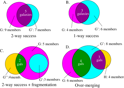
Figure 4.— Schematic depiction of various success and failure modes for group-finding under the criteria discussed in the text. Diagrams show hypothetical comparisons between real groups (unprimed) and the groups found by a group finder (primed). (A) A fully two-way successful reconstruction, in which both the real and found group have $\mathcal{L}_{G}>0.5$. (B) A one-way success, in which the real group has $\mathcal{L}_{G}>0.5$, but half of the found group is made up of interlopers. (C) Both a two-way success ($G$ and $G^{\prime}$) and a failure due to fragmentation ($G^{\prime\prime}$). (D) An example of overmerging, in which $G$ and $H$ are both one-way successful real groups, but $G^{\prime}$ combines their members into a single group.

The LGF statistic allows us to define an unambiguous set of group-finding success measures. In essence, we declare a successful detection if a group’s $\mathcal{L}_{G}$ is greater than some fraction $f$. For this definition to be unique, we must have $f\geq 0.5$, with higher values of $f$ implying a more stringent definition of success. For the remainder of this work, we will set $f$ to the minimal value of $0.5$, since, as we shall see, this definition of success is already quite strict. However, simply requiring a group to have $\mathcal{L}_{G}>f$ is insufficient: a real group could meet this criterion but still been merged into a larger object by the group-finder, and a reconstructed group $G^{\prime}$ could have $\mathcal{L}_{G^{\prime}}>f$ if it is a fragment of a larger real group. For this reason, it will be important to differentiate between one-way matches, in which a group simply has LGF above $f$, and two-way matches, in which a group $G$ and its LAG $G^{\prime}$ satisfy $\mathcal{L}_{G},\mathcal{L}_{G^{\prime}}>f$, and $G$ is also the LAG of $G^{\prime}$ (See Figure 4 for a schematic depiction of these success measures). Hence we shall differentiate between one-way purity $P_{1}$, the fraction of reconstructed groups with $\mathcal{L}_{G}>f$, and two-way purity $P_{2}$, the fraction of reconstructed groups which are two-way matches with some real group. Similarly, for real groups, we define one-way completeness $C_{1}$ and two-way completeness $C_{2}$. Comparing these statistics can give some indication of systematic errors in the group catalog. A real group that is a one-way success but not a two-way success has likely been overmerged by the group finder; therefore if $C_{1}$ is much larger than $C_{2}$ we expect that our catalog has been highly over-merged. Similarly, if $P_{1}$ is significantly greater than $P_{2}$, we expect that our catalog is highly fragmented.

Our definition of success has another potential problem, however: it requires, minimally, only that we reconstruct half of each group. Thus, a “successful” search strategy could seek only the most tightly clustered sets of galaxies and detect only the cores of groups and clusters. Such a group catalog would likely be of high purity, with few interlopers; it could be useful for identifying groups for follow-up observation in X-ray or Sunyaev-Zeldovich surveys. But it would likely have low completeness, and it probably would not accurately reproduce group properties like richness, physical size, or velocity dispersion, making estimates of cluster mass impossible with spectroscopic data alone.

In order to mitigate such difficulties, we must also monitor our success in reproducing group properties. In part, this means we should attempt to accurately measure properties like the velocity dispersion of successfully reconstructed groups on a group-by-group basis. However, since errors in individual group detections are inevitable with any group finder, we must also determine whether these errors bias the overall distribution of group properties in our catalog. Ultimately it is these statistical distributions we will want to reproduce as accurately as possible. For example, if we wish to study the abundance of groups as a function of redshift, $n(z)$, we must take care to ensure that spurious group detections and undetected real groups do not skew this distribution.

Clearly, then, there are many different possible means by which we could gauge our success at group finding. As we have said, our chosen measure of success will depend strongly on the ultimate scientific purposes of our group catalog. In our case, among other uses, we envision using the DEEP2 group catalog to constrain cosmological parameters. Newman et al. (2002) have shown that DEEP2 groups can be used for this purpose if their abundance is measured accurately as a bivariate distribution in velocity dispersion and redshift, $n(\sigma,z)$. It has also been shown (Marinoni et al. 2002) that the Voronoi-Delaunay group-finding algorithm can successfully reconstruct this distribution (down to some limiting velocity dispersion $\sigma_{c}$); hence we will seek in this study to maximize the accuracy of our reconstructed $n(\sigma,z)$ above some $\sigma_{c}$. Of course, it would be possible in principle to reproduce this distribution by chance with a low-purity, low completeness catalog. Therefore, we will simultaneously strive to maximize the completeness and purity parameters, while also taking care to keep $C_{1}\approx C_{2}$ and $P_{1}\approx P_{2}$ to guard against fragmentation and over-merging. Indeed, it is always important to monitor these statistics in order to ensure that our reconstructed group catalog corresponds reasonably well with reality. We do not actively monitor the $S_{Gal}$ or $f_{I}$ parameters when optimizing our group finder, but we anticipate that a catalog that meets our success criteria will also be of reasonably high quality by these measures as well (this is borne out in Section 4.3).

In concluding this section, it is important to note that when we speak of group velocity dispersions or redshifts in this paper, we are talking only about the properties as computed from the observed group members. Although we will ultimately be interested in the properties of dark matter halos (which can be predicted theoretically and used to constrain cosmology), these cannot be measured directly, even in principle. Even with a completely error-free group catalog, a theoretical correction would have to be applied to account for the effects of discreteness. Thus we will be interested in reconstructing $n(\sigma,z)$ as computed using observed galaxies only. We make no attempt to reconstruct the distribution as computed for the dark matter or using unobserved galaxies, and we leave computation of theoretical correction factors to future work.

4. Choosing and optimizing the group-finder

Several different techniques have been developed to find groups in spectroscopic redshift samples. We review them briefly here, as a means of introducing the main issues that will concern us in selecting a group-finding algorithm.

4.1. A brief history of group finding

Huchra & Geller (1982) presented a simple early method for identifying groups and clusters in the Center for Astrophysics (CfA) redshift survey by looking for nearby neighbor galaxies around each galaxy. Commonly known as the friends of friends or percolation method, this technique, in its simplest form, defines a linking length $b$ and links every galaxy to those neighboring galaxies a distance $b$ or less away (“friends”). This procedure produces complexes of galaxies linked together via their neigbors (“friends of friends”); these complexes are identified as groups and clusters. Versions of this algorithm have been widely used to identify groups in local redshift surveys—most recently by Eke et al. (2004) in 2dFGRS—and percolation techniques have also long been used to identify virialized dark-matter halos within N-body simulations. The percolation algorithm is intuitively attractive because it identifies those regions with an overdensity $\delta\geq(2\pi b^{3}/3)^{-1}$ compared to the background density. The overdensity $\delta_{v}$ of virialized objects can be readily computed using the well-known spherical collapse model, yielding an appropriate linking length of $b=0.2\langle\nu\rangle^{-1/3}$ for identifying virialized objects in an Einstein-de Sitter universe (Davis et al. 1985), where $\langle\nu\rangle$ is the mean spatial number density of galaxies (this linking length is somewhat smaller for a $\Lambda$CDM model, a point which has frequently been ignored in the literature). Hence, the percolation algorithm is a natural method for identifying virialized structures in the absence of redshift-space distortions.

Unfortunately, working in redshift space can cause serious problems for this algorithm. The fingers-of-God effect requires that we stretch the linking volume into an ellipsoid or cylinder along the line of sight, which increases the possibility of spurious links. Because the percolation method considers each galaxy equally while creating links, then places all linked galaxies into a given group or cluster, such false links can lead to catastrophic failures, in which the group finder “hops” between several nearby groups, merging them together into a single, falsely detected massive cluster. On the other hand, shrinking the linking volume to avoid this problem increases the chances that a given structure will be fragmented into several smaller structures by the group finder or missed entirely. These problems have been studied in detail by Nolthenius & White (1987) and more recently by Frederic (1995).

To combat such difficulties, various other group-finding methods have been developed. Tully (1980, 1987) used the so-called “hierarchical” group-finding scheme, originally introduced by Materne (1978), to find nearby groups. The hierarchical grouping procedure used is computationally interesting, but in the context of the current model of structure formation it seems to lack theoretical motivation. More recently, the SDSS team has introduced a group-finding algorithm called C4 (Nichol 2004), which searches for clustered galaxies in a seven-dimensional space, including the usual three redshift-space dimensions and four photometric colors, on the principle that galaxy clusters should contain a population of galaxies with similar observed colors. Kepner et al. (1999) introduced a three-dimensional “adaptive matched filter” algorithm which identifies clusters by adding “halos” to a synthesized background mass density and computing the maximum-likelihood mass density. White & Kochanek (2002) found that this algorithm is extremely successful at identifying clusters in spectroscopic redshift surveys, and recently, Yang et al. (2004) have introduced a group-finder that combines elements of the matched filter and percolation algorithms. Finally, Marinoni et al. (2002) developed a group-finding algorithm—the Voronoi-Delaunay Method (VDM)—that makes use of the Voronoi partition and Delaunay triangulation of a galaxy redshift survey to identify high-density regions. By performing a targeted, adaptive search in these regions, the VDM avoids many of the pitfalls of simple percolation methods; we will use a version of it in this study. We note in passing, however, that the matched-filter algorithm is also attractive for DEEP2, and we plan to explore its usefulness in future studies.

4.2. The Voronoi-Delaunay method

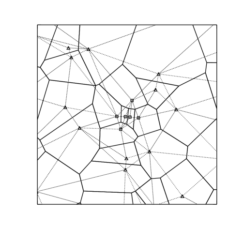
Figure 5.— The two-dimensional Voronoi partition (Dirichlet tesselation) and Delaunay mesh for an array of points. The points consist of a randomly generated uniform background (triangles) and a small, tightly clustered group of points (squares) that roughly approximate a galaxy group. Dotted lines show the Delaunay mesh, which connects each point to its nearest neighbors. The solid lines delineate the edges of the Voronoi polygons—the perpendicular bisectors of the Delaunay links. Note that each polygon contains only one point, and that the typical Voronoi cell is smaller for the grouped points than for the background points.

Marinoni et al. (2002) showed that the VDM successfully reproduces the distribution of groups in velocity dispersion in a DEEP2-like sample down to some minimum dispersion $\sigma_{c}$. The algorithm makes use of the three-dimensional Voronoi partition of the galaxy redshift catalog, which tiles space with a set of unique polyhedral sub-volumes, each of which contains exactly one galaxy and all points closer to that galaxy than to any other. The Voronoi partition naturally provides information about the clustering properties of galaxies, since galaxies with many neighbors will have small Voronoi volumes, while relatively isolated galaxies will have large Voronoi volumes. The algorithm also makes use of the clustering information encoded in the Delaunay mesh, which is a complex of line segments linking neighboring galaxies. Mathematically speaking, the Delaunay mesh is the geometrical dual of the Voronoi partition; the faces of the Voronoi cells are the perpendicular bisectors of the lines in the Delaunay mesh. A two-dimensional visual representation of the Voronoi partition and Delaunay mesh is shown in Figure 5.

The VDM group-finding algorithm proceeds iteratively through the galaxy catalog in three phases as follows. In Phase I, all galaxies that have not yet been assigned to groups are sorted in ascending order of Voronoi volume. This is mainly a time-saving step, because it allows us to begin our group search with those galaxies in dense regions. Then, for the first galaxy in this sorted list (the seed galaxy), we define a relatively small cylinder of radius $\mathcal{R}_{\mathrm{min}}$ and length $2\mathcal{L}_{\mathrm{min}}$, oriented with its axis along the redshift direction. The dimensions of this and other search cylinders are computed using comoving coordinates. Within this cylinder, we find all galaxies that are connected to the seed galaxy by the Delaunay mesh (the first-order Delaunay neighbors). If there are no such galaxies, the seed galaxy is said to be isolated, and the algorithm moves on to the next seed galaxy in the list. By initially searching in a small cylinder, we are able to limit the probability of chance associations being misidentified as groups.

If, however, there are one or more first-order Delaunay neighbors, we move on to Phase II. We define a second, larger cylinder, concentric with the first one, with radius $\mathcal{R}_{II}$ and length $2\mathcal{L}_{II}$. Within this cylinder, we identify all galaxies that are connected to the seed galaxy or to its first-order Delaunay neighbors by the Delaunay mesh. These are the second-order Delaunay neighbors. The seed galaxy and its first- and second-order Delaunay neighbors constitute a set of $N_{II}$ galaxies; we take $N_{II}$ to be an estimate of the central richness of the group. Scaling relations are known to exist between group mass and radius and velocity dispersion (Bryan & Norman 1998), and between velocity dipsersion and central richness (Bahcall 1981). Thus we may estimate the final size of the group from $N_{II}$. In particular, we expect that $N_{II}\propto M\propto\sigma^{3}\propto R^{3}$.

Therefore in Phase III we define a third cylinder, centered on the center of mass of the $N_{II}$ galaxies from Phase II, with radius and half-length given by

$$\mathcal{R}_{III} = r(N_{II}^{corr})^{\frac{1}{3}}$$ (3)

$$\mathcal{L}_{III} = \ell(N_{II}^{corr})^{\frac{1}{3}},$$

where $r$ and $\ell$ are free parameters that must be optimized. Here, the corrected central richness $N_{II}^{corr}$ is scaled to account for the redshift-dependent number density $\nu(z)$ of galaxies in a magnitude-limited survey:

$$N_{II}^{corr}=\left(\frac{\langle\nu(z)\rangle}{\langle\nu(0.7)\rangle}\right)^{-1}N_{II}.$$ (4)

We compute $\langle\nu(z)\rangle$ by smoothing the redshift distribution of the entire galaxy sample and dividing it by the differential comoving volume element $dV/dz$ to yield the comoving number density. All galaxies within the Phase III cylinder (and any of the $N_{II}$ galaxies from Phase II that happen to fall outside of it) are taken to be members of the group. After a group has been identified, this three-phase process repeated on all remaining galaxies that have not yet been assigned to groups until all galaxies have either been placed into groups or explicitly identified as isolated galaxies.

The astute reader may object here that we have used the central richness $N_{II}$ to scale our search window, even though we found earlier that richness is a relatively unstable group property within the DEEP2 sample. This is true. However, the groups in our mock catalogs do show some correlation between actual and observed richness, even though the scatter is very large. Furthermore, we have mitigated one major source of error, Malmquist bias, with the correction in equation 4. Since the dependence of our scaling on $N_{II}$ is relatively weak, we anticipate that errors in estimating this quantity will not introduce insurmountably large errors into our group sample. This expectation is borne out by tests on mock catalogs, as will be seen in Section 4.3.

Finally, it is important to note some minor differences between our group-finder and the one described in Marinoni et al. (2002). In that paper, the scaling factors $r$ and $v$ in Equation 3 were derived iteratively by running the group-finder first with a best-guess parameter set and then automatically adjusting parameters according to the largest groups found. In tests on mock catalogs, we found this method to be unstable, so we instead choose to optimize our parameters empirically with mock catalogs and then leave them fixed. Also, when we search for groups in cylinders, it is important to note that the “length” of our cylinders is supposed to correspond to an expected maximum velocity of the galaxies in the group. Since the mapping between redshift interval and peculiar velocity changes with redshift, we must rescale the length of our search cylinders as $\mathcal{L}(z)=[s(z)/s(z_{0})]\mathcal{L}_{0}$, where the scaling factor $s(z)$ is given by

$$s(z)=\frac{1+z}{\sqrt{\Omega_{M}(1+z)^{3}+\Omega_{\Lambda}}}$$ (5)

for the standard $\Lambda$CDM cosmology. This scaling amounts to a $\sim 10\%$ effect over the redshift range of the DEEP2 survey. We apply it to the cylinder in each phase, taking a reference redshift of $z_{0}=0.7$.

4.3. Optimizing with mock catalogs

To gauge the success of our group-finding algorithm, we will make use of the mock DEEP2 sample described in Section 2.2. Each galaxy in these catalogs is tagged with the name of its parent halo, making the identification of real groups a simple matching exercise. Thus, we have a catalog of real groups, identified from N-body models in real space, against which we can compare the results of applying the VDM algorithm to the mock galaxy catalog projected in redshift space. To compute completeness and purity, we simply apply equation (2) to the real and reconstructed group catalogs.

As a rough measure of the accuracy of our reconstructed distribution, $n_{\mathrm{found}}(\sigma,z)$, we apply a two-dimensional Kolmogorov-Smirnov (K-S) test to this distribution and the real distribution, $n_{\mathrm{real}}(\sigma,z)$, to determine whether they are statistically distinguishable. Marinoni et al. (2002) found that the VDM group-finder should accurately reproduce this distribution above $\sigma_{c}\approx 400\mathrm{\;km\;s^{-1}}$, so we apply the K-S test only above this velocity dispersion. The test is insensitive to the total number of groups in each sample, so we must independently ensure that the two distributions have the same normalization. To do this, we simply count the total number of groups with $\sigma\geq 400\mathrm{\;km\;s^{-1}}$. We want to ensure that the real and reconstructed normalizations match to better than the expected cosmic variance for our sample (about $12\%$ for the abundance of groups with $\sigma\geq 400\mathrm{\;km\;s^{-1}}$), so that our final errors are dominated by cosmic variance. Guided by simple physical considerations (e.g., the expected velocity dispersion range of groups and clusters), we explore the space of VDM parameters $\mathcal{R}_{\mathrm{min}},\mathcal{L}_{\mathrm{min}},\mathcal{R}_{\mathrm{II}},\mathcal{L}_{\mathrm{II}},r$ and $\ell$, using trial and error to narrow our parameter range down to a range that produces an $n_{\mathrm{found}}(\sigma,z)$ that is statistically indistinguishable from $n_{\mathrm{real}}(\sigma,z)$ (less than 1% confidence that the two distributions are different) and properly normalized. At the same time, we monitor the completeness and purity of the reconstructed group catalog requiring, minimally, that $C_{2}$ and $P_{2}$ remain above $50\%$ and attempting to increase them as much as possible.

The procedure described above is simple to implement and perform; however, it is ultimately an insufficient test of our success. It asks only whether or not $n_{\mathrm{found}}(\sigma,z)$ and $n_{\mathrm{real}}(\sigma,z)$ appear, in a statistical sense, to have been drawn from the same distribution. But we want to know whether or not $n_{\mathrm{found}}(\sigma,z)$ is an accurate reconstruction of $n_{\mathrm{real}}(\sigma,z)$; for the two distributions to pass a K-S test is a necessary but not a sufficient condition. In order to fully optimize our parameters, we must aim to reduce any systematic error in $n_{\mathrm{found}}-n_{\mathrm{real}}$ to a level below the cosmic variance.

Thus, we will want to assess our error in reconstructing the acutal velocity function $n_{\mathrm{real}}(\sigma,z)$ in a given field, irrespective of cosmic variance, and then compare our reconstruction error to the expected cosmic variance in that field. As long as the systematic error is smaller than the cosmic variance, it will not be a significant source of error in our measurement of the velocity function. To estimate our systematic error, we apply the VDM group finder to twelve independent DEEP2 fields and compute the mean fractional residuals $\langle\delta_{n}\rangle\equiv\langle(n_{\mathrm{found}}-n_{\mathrm{real}})/n_{\mathrm{found}}\rangle$, which constitute a measurment of the fractional systematic reconstruction error. The uncertainty in determining $\langle\delta_{n}\rangle$ is then given by the standard error in this quantity, $\sigma_{\langle\delta\rangle}$. We have used fractional errors here, rather than absolute errors, to distinguish errors in reconstruction from the intrinsic scatter (cosmic variance) in $n_{\mathrm{real}}$ and $n_{\mathrm{found}}$. We can then measure the fractional cosmic variance (plus Poisson noise) $\sigma_{cos}\equiv(\langle n_{\mathrm{real}}^{2}\rangle/\langle n_{\mathrm{real}}\rangle^{2}-1)^{1/2}$ from the mock catalogs and compare it to the systematic error $\langle\delta_{n}\rangle$.

Table 2Parameters used for group finding with the VDM algorithm in this study.

Parameter	Optimal	High-purity
$\mathcal{R}_{min}$	0.3	0.1
$\mathcal{L}_{min}$	7.8	5.0
$\mathcal{R}_{II}$	0.5	0.3
$\mathcal{L}_{II}$	6.0	5.0
$r$	0.35	0.25
$\ell$	14	14

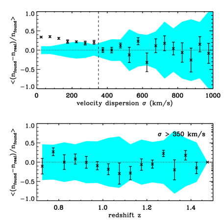
Figure 6.— Fractional errors in measuring $n(\sigma)$ and $n(z)$. Upper panel: the data points show the fractional systematic error $\langle\delta_{n}\rangle$ as a function of velocity dispersion, estimated by running the VDM algorithm on twelve independent mock DEEP2 pointings. Error bars show the standard deviation of the mean $\sigma_{\langle\delta\rangle}$, while the shaded region (light blue in the electronic edition) shows the fractional cosmic variance (plus Poisson noise) $\sigma_{cos}$ for a single ($120\times 30$ arcmin) DEEP2 field, in bins of $50\mathrm{\;km\;s^{-1}}$. For $\sigma\gtrsim 350\mathrm{\;km\;s^{-1}}$, the systematic errors are dominated by cosmic variance. Bottom panel: Fractional errors in $n_{\mathrm{found}}$ and fractional cosmic variance, as a function of redshift in bins of 0.05 in $z$, after groups with $\sigma<350\mathrm{\;km\;s^{-1}}$ have been discarded. Any systematic offsets are smaller than the cosmic variance.

For simplicity of presentation, we first consider the integrated one-dimensional distributions $n(\sigma)$ and $n(z)$. Figure 6 shows the fractional systematic errors $\langle\delta_{n}\rangle$ in these distributions, and error bars show the uncertainty $\sigma_{\langle\delta\rangle}$ in determining this quantity. These two quantities are measured by applying the VDM group-finder to the DEEP2 mock catalogs using the “optimal” VDM parameter set shown in Table 2. Also shown is the fractional cosmic variance (plus Poisson noise) $\sigma_{cos}$ expected in a single ($120\times 30$ arcmin) DEEP2 field. As shown in the upper panel of the figure, systematic reconstruction errors in $n_{\mathrm{found}}(\sigma)$ are dominated by cosmic variance for $\sigma>350\;\mathrm{\;km\;s^{-1}}$, while we significantly overestimate the abundance of lower-dispersion groups. If we discard the reconstructed groups with $\sigma<350\;\mathrm{\;km\;s^{-1}}$, systematic errors in the $n_{\mathrm{found}}(z)$ distribution are also smaller than the cosmic variance, as shown in the bottom panel of the figure. We note that we have been able to do somewhat better than expected, reconstructing the velocity function accurately down to $\sigma=350\mathrm{\;km\;s^{-1}}$, slightly lower than the cutoff of $400\mathrm{\;km\;s^{-1}}$ expected from Marinoni et al. (2002).

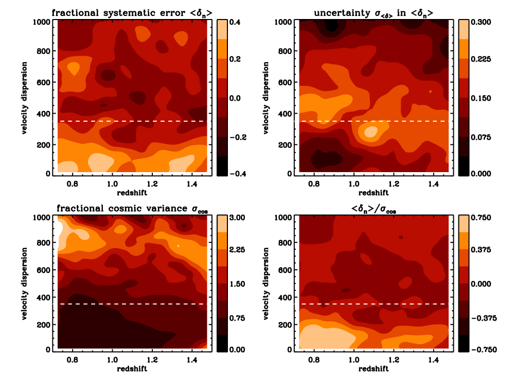
Figure 7.— Contour plots of the error statistics for the two-dimensional distribution $n(\sigma,z)$, where the binning in each dimension is the same as in figure 6 and the error distributions have been smoothed by one bin in each direction for cleaner presentation. Upper left: The mean fractional systematic error $\langle\delta_{n}\rangle$ in each bin, computed by applying the VDM group finder to twelve independent mock DEEP2 pointings. Upper right: The standard deviation of the mean $\sigma_{\langle\delta\rangle}$ amongst the 12 mock catalogs for the quantity shown in the upper left panel. Lower left: The fractional cosmic variance (plus Poisson noise) $\sigma_{cos}$ in each bin, estimated from the same twelve mock pointings. Lower right: The ratio of mean fractional systematic error error to fractional cosmic variance. In each panel, contour values are indicated by color bars. Significant systematic errors in the measured distribution are confined to small velocity dispersions, while for $\sigma\gtrsim 350\mathrm{\;km\;s^{-1}}$ the errors are dominated by cosmic variance, with no large-scale bin-to-bin correlations. In each panel, the dashed line indicates $\sigma=350\mathrm{\;km\;s^{-1}}$ for reference.

The fact that these one-dimensional distributions are accurately measured to within the cosmic variance is heartening, but to fully optimize our group-finder we must ensure that the full two-dimensional distribution $n(\sigma,z)$ is accurately measured. Figure 7 shows smoothed contour plots of the mean fractional systematic errors $\langle\delta_{n}(\sigma,z)\rangle$ in this distribution, the uncertainty $\sigma_{\langle\delta\rangle})$ in this quantity, the fractional cosmic variance $\sigma_{cos}$, and the ratio of the systematic error to the cosmic variance. The panel at the lower right shows that significant, correlated overestimates of the distribution are confined to low velocity dispersion. For $\sigma\gtrsim 350\mathrm{\;km\;s^{-1}}$, on the other hand, the errors are smaller than the cosmic variance and exhibit no systematic, large-scale bin-to-bin correlations.

To be somewhat more quantitative, we note that for $\sigma\geq 350\mathrm{\;km\;s^{-1}}$, the average value of the ratio $(\langle\delta_{n}\rangle/\sigma_{cos})^{2}$ shown in the lower right panel of Figure 7 (before smoothing) is 0.1, and the maximum value is 0.9. Thus we may proceed with confidence that $n(\sigma,z)$ for DEEP2 is reconstructed with sufficient accuracy by the VDM group-finder for velocity dispersions above $350\mathrm{\;km\;s^{-1}}$. Therefore, having achieved our optimization goals, we may apply the VDM algorithm to the DEEP2 redshift catalog with confidence that our reconstructed catalog will produce an accurate and unbiased measurement of $n(\sigma,z)$ for $\sigma>350\mathrm{\;km\;s^{-1}}$ (as long as our mock catalogs are a reasonable representation of the real universe). We note that this minimum velocity dispersion is not a limitation of the VDM group-finder—a more densely sampled survey would permit $n(\sigma,z)$ to be reconstructed down to even lower dispersions (Marinoni et al. 2002). More generally, it is important to recognize that the conclusions reached here apply only to the DEEP2 survey: a survey probing significantly greater volume, for example, would have smaller cosmic variance, perhaps necessitating a more accurate reconstruction of $n(\sigma,z)$ than has been presented here.

Figure 8.— Completeness and purity statistics as a function of velocity dispersion for the optimized VDM group-finder. Crosses show the mean one-way statistics $C_{1}$ and $P_{1}$ (see Section 3 for definitions), in bins of $50\;\mathrm{\;km\;s^{-1}}$, as obtained from running the group-finder on the twelve independent mock catalogs. Squares show the mean two-way statistics $C_{2}$ and $P_{2}$. Error bars indicate the standard deviation of the mean for each statistic in each bin.

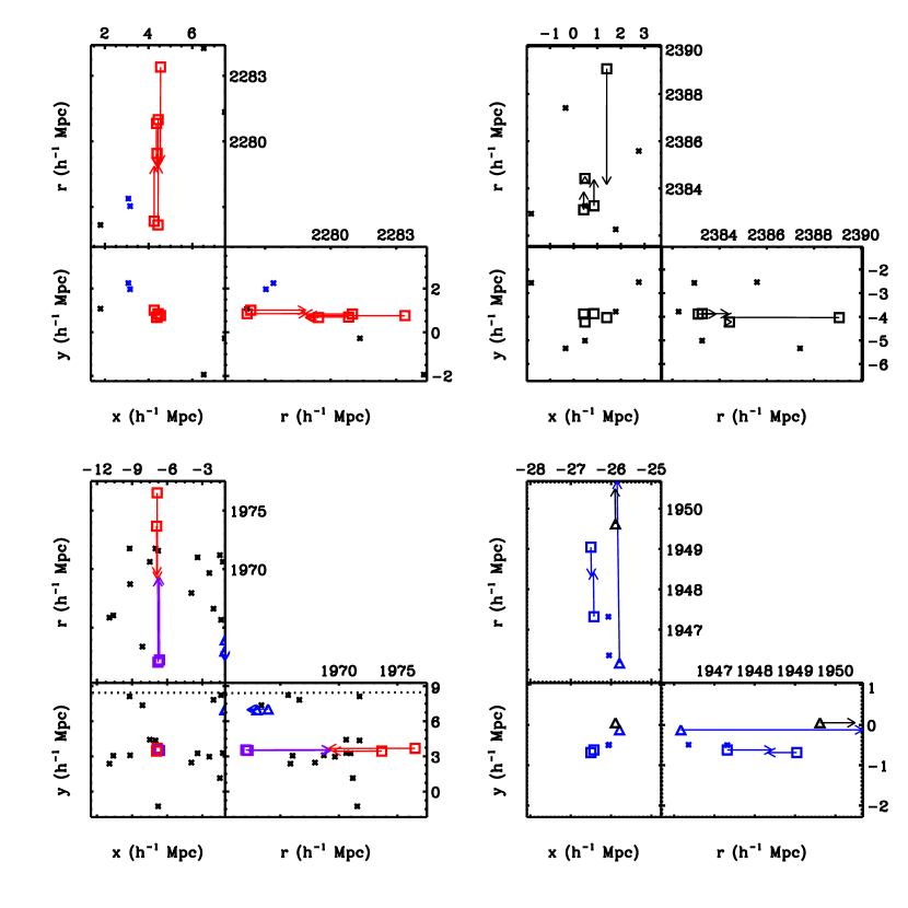
Figure 9.— Examples of group-finding success and failure in the DEEP2 mock catalogs. In each panel, squares indicate galaxies in the real group being plotted, triangles indicate galaxies in nearby real groups, and crosses indicate nearby field galaxies. Galaxies are plotted both as seen on the sky and in twod line-of-sight projections in redshift space. Arrows point to the galaxies’ real space positions, to show the effects of redshift-space distortions (to reduce visual clutter, no arrows are plotted for field galaxies). Dotted lines indicate field edges. Each reconstructed group is indicated by a different shade (color in the electronic edition), with reconstructed field galaxies shown in black. The upper left panel shows a perfect reconstruction with a nearby false detection; the upper right panel shows a completely undetected group (all black squares); the lower left panel shows a fragmented real group; and the lower right panel shows an example of overmerging.

After running the VDM on the 12 mock samples using the optimal parameter set in Table 2, we obtain mean completeness parameters of $C_{1}=0.782\pm 0.006$ and $C_{2}=0.719\pm 0.005$ and mean purity parameters of $P_{1}=0.545\pm 0.005$ and $P_{2}=0.538\pm 0.005$, with the quoted uncertainties indicating the standard deviations of the means. As shown in Figure 8, these statistics are nearly independent of the velocity dispersion of the groups being considered. The fact that $C_{1}-C_{2}$ and $P_{1}-P_{2}$ are small suggests that our catalogs are largely free of fragmentation or over-merging. We also find that most galaxies that belong to real groups are identified as group members: the mocks yield a mean galaxy-success rate of $S_{Gal}=0.786\pm 0.006$. Conversely, the mean interloper fraction is $f_{I}=0.458\pm 0.004$, indicating that the galaxies in our reconstructed group catalogs are dominantly real group members.

Since the purity is relatively low, it will be difficult to know whether to believe in the reality of any individual group in our optimal group sample, although the properties of the catalog as a whole are accurately measured. To give some sense of the errors encountered in reconstructing individual groups, we show several examples of group-finding success and failure in Figure 9. In order to produce a catalog that may be believed with more confidence on a group-by-group basis, we can optimize the VDM parameters to maximize the purity (contingent on the requirement that we still find an appreciable number of groups). The high-purity parameter set shown in Table 2 gives mean purity measures in the mock catalogs of $P_{1}=0.825\pm 0.007$ and $P_{2}=0.815\pm 0.006$. The completeness measures are necessarily much lower for this parameter set, however: $C_{1}=0.284\pm 0.008$ and $C_{2}=0.277\pm 0.008$.

5. The first DEEP2 group catalog

We have applied the VDM group finding algorithm to galaxies in the three most completely observed DEEP2 pointings using the optimal parameters from Table 2. Figures 10 and 11 show groups found in pointing 32 (see Table 1), both as seen on the sky, and as seen along the line of sight, projecting through the shortest dimension of the field. Especially notable in these diagrams is the clear visual confirmation that groups are strongly biased tracers of the underlying dark matter distribution. The groups we find clearly populate dense regions and filaments preferentially in these figures. Close-up views of a few of the larger groups from this pointing can be seen in Figure 12.

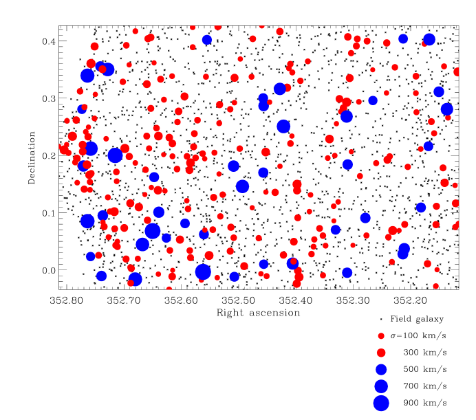
Figure 10.— Groups as seen on the sky in DEEP2 pointing 32 (see Table 1). In this figure, group-member galaxies have been removed, and the median positions of groups are indicated by colored circles with diameter proportional to measured velocity dispersion, as shown in the legend. Groups with $\sigma<350\mathrm{\;km\;s^{-1}}$ are indicated in light gray (red in the electronic edition), while groups with $\sigma\geq 350\mathrm{\;km\;s^{-1}}$ are shown in dark gray (blue). The positions of field galaxies are indicated by black dots.

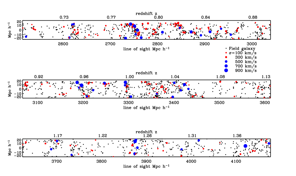
Figure 11.— Groups of galaxies in DEEP2 pointing 32 as seen along the line of sight from the observer, projecting through the shortest dimension of the field. Symbols are as in Figure 10. Line-of-sight distances have been computed using a flat flat $\Lambda$CDM cosmology with $\Omega_{M}=0.3$ and equation of state $w=-1$. Note that these groups are strongly biased: they trace out the densest large-scale structures in the survey.

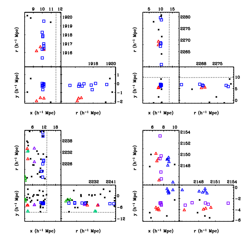
Figure 12.— Close-up views of four DEEP2 groups. Shaded squares (colored in the electronic edition) indicate galaxies in the group being considered, shaded (colored) triangles indicate galaxies in nearby groups, and black crosses indicate nearby field galaxies. Each group is shown in three projections: one as seen on the sky and two along the line of sight.

Our optimal VDM group-finder identifies a total of 899 groups with $N\geq 2$ in the three fields considered here, with $32\%$ of all galaxies in the sample being placed into groups. We note that this percentage is much lower than that found in the 2dFGRS by Eke et al. (2004) ($55\%$); however, our observational selection criteria and group-finding methods are sufficiently different from theirs that detailed comparisons will be quite difficult. By comparing the volume of the initial search cylinder used in Phase I of the VDM group-finder to the number density of DEEP2 galaxies in the range $0.7\leq z<0.8$, we estimate that our groups have a minimum central overdensity (in redshift space) of $\delta\nu/\nu\gtrsim 100$.

In Table 3 we present the locations and properties of the subset of groups with $\sigma\geq 350\mathrm{\;km\;s^{-1}}$ (153 groups). We also have found groups in the same data using the high-purity parameter set in Table 2. We can match our two group catalogs by identifying those groups in the optimal catalog that are the Largest Associated Groups of the groups in the high-purity catalog. Such groups are noted as “strong” detections in Table 3; they are highly likely ($>80\%$ chance) to be associated with real virialized structures. Such strong detections constitute $17\%$ of the total group sample and $13\%$ of the sample with $\sigma\geq 350\mathrm{\;km\;s^{-1}}$.

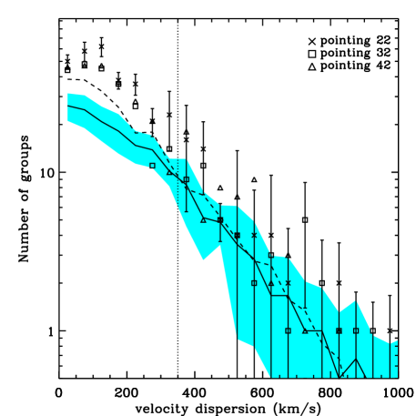
Figure 13.— Comparison of the velocity function $n(\sigma)$ measured in a three DEEP2 pointings (see Table 1) to that predicted by mock catalogs. The data points are the measured velocity function, in bins of $50\mathrm{\;km\;s^{-1}}$, of groups found in the three pointings. Error bars are estimated by applying the VDM group finder to twelve independent mock DEEP2 pointings, measuring $n(\sigma)$, and taking the standard deviation of the fractional residuals $\delta_{n}$ to estimate a fractional error in each bin. For clarity, error bars are only shown for one data point in each bin. The solid line is the average “true” velocity function from the mock DEEP2 catalogs (see Section 2.2), $\langle n_{\mathrm{true}}(\sigma)\rangle$, in bins of $50\mathrm{\;km\;s^{-1}}$, and the shaded region (light blue in the electronic edition) indicates the combined cosmic variance and Poisson noise in each bin, for a single DEEP2 pointing. The dashed line shows the average reconstructed velocity function, $\langle n_{\mathrm{found}}(\sigma)\rangle$. The measured velocity function is consistent with the mock catalogs in the regime $\sigma>350\mathrm{\;km\;s^{-1}}$ (demarcated by the dotted line), where an accurate measurement is expected.

Throughout this study, we have focused on reconstructing a group catalog that provides an accurate measure of the velocity function $n(\sigma)$. The ultimate goal of measuring cosmological parameters must wait for more data, but it is interesting at this stage to compare the DEEP2 data to the predictions from mock catalogs. Figure 13 compares the measured velocity function $n(\sigma)$ (data points) to the true velocity function $n_{\mathrm{true}}(\sigma)$ (solid line) predicted by the mock DEEP2 sample described in Section 2.2. The measured velocity functions are qualitatively consistent with the prediction from the mock catalogs for $\sigma\gtrsim 350\mathrm{\;km\;s^{-1}}$, while the measurements are significantly higher than the prediction for lower velocity dispersions. In Section 4.3, we showed that an accurate reconstruction of the velocity function is expected in the higher-dispersion regime, while an overestimate of $n(\sigma)$ is expected at lower velocity dispersions. We intend to exclude low-dispersion groups from future analyses, so we do not consider the high measured values for $n(\sigma)$ a particular cause for concern.

However, it is important to note that this comparison—of the measured velocity function to the “true” velocity function in the mock catalogs—is not, strictly speaking, the appropriate comparison to make to assess the similarity of the mocks and the data. A real “apples-to-apples” comparison would compare the measured $n(\sigma)$ to the mean reconstructed velocity function $\langle n_{\mathrm{found}}(\sigma)\rangle$ derived by applying the VDM group-finder to all twelve mocks. This quantity is indicated by the dashed line in Figure 13; the data appear to be consistent with it at velocity dispersions $\sigma\gtrsim 300\mathrm{\;km\;s^{-1}}$.

Below this threshold a slight discrepancy remains: the data points lie significantly above the dashed line at low dispersions. However, one would naively expect the velocity function reconstructed from the data to be everywhere consistent with the one reconstructed in the mock catalogs, if the mocks are a good simulation of the data. It is difficult to assess the significance of the discrepancy shown here, since we have not optimized our group-finder to measure the abundance of such low-dispersion groups, but it appears that the the mock catalogs may be inconsistent with the DEEP2 data on small velocity scales. Nevertheless, it is clear that the mocks are consistent with the data in the high-dispersion regime, so this comparison confirms that the mock catalogs are an accurate simulation of DEEP2 data for our purposes. The more scientifically interesting “data-to-prediction” comparison shown by the solid line in Figure 13 then stands as evidence that an accurate reconstruction of the velocity function for $\sigma>350\mathrm{\;km\;s^{-1}}$ is possible in DEEP2, providing the first step necessary to placing constraints on cosmological parameters.

6. Discussion and Conclusions

We have optimized the VDM group-finding algorithm using mock catalogs designed to replicate the DEEP2 survey, and we have applied it to spectroscopic data from three DEEP2 photometric pointings. In the process of optimization, we have defined a measure of group finding success that focuses on accurately reproducing the overall properties of the group catalog—in particular the distribution of groups in redshift and velocity dispersion, $n(\sigma,z)$—while paying some attention also to the accurate reconstruction of individual groups. Tests on DEEP2 mock catalogs show that we are able to accurately reproduce $n(\sigma,z)$ for $\sigma\geq 350\mathrm{\;km\;s^{-1}}$ and that errors in measuring this quantity in DEEP2 should be smaller than its expected intrinsic cosmic variance. It should thus be possible to use the test described by Newman et al. (2002) to constrain cosmological parameters, including the dark energy equation of state parameter, $w$.

We find 899 groups with two or more members within the DEEP2 data considered in this study, roughly $25\%$ of the expected final sample. Of these, 153 have velocity dispersions $\sigma\geq 350\mathrm{\;km\;s^{-1}}$. The distribution of these reconstructed groups with velocity dispersion $n(\sigma)$ is in good agreement with the distribution for real groups in DEEP2 mock catalogs. This result provides a useful consistency check for the mock catalogs: assuming our reconstructed $n(\sigma)$ is accurate (as our tests show that it is for $\sigma\geq 350\mathrm{\;km\;s^{-1}}$), we may be confident that the properties of groups in the mock catalogs are an accurate simulation of real DEEP2 data. This is especially important in the context of the so-called velocity bias, which is the ratio of the velocity dispersion of galaxies to that of the underlying dark matter halo, $b_{v}=\sigma_{\mathrm{gal}}/\sigma_{\mathrm{DM}}$. Various studies of N-body simulations (e.g., Diemand et al. 2004, and references therein) have suggested that $b_{v}\neq 1$ at the 15–30% level, but no such effects have been included in the DEEP2 mock catalogs. Our results on $n(\sigma)$ thus indicate that our data are consistent with $b_{v}=1$ within the measurement errors shown in Figure 13. This is no surprise, since our current error bars are considerably larger than the expected effect; nevertheless, this result may be viewed as confirmation that no stronger biases exist.

Successful detection of groups and clusters within the DEEP2 redshift survey is an essential first step for a wide variety of planned studies. By comparing the properties of galaxies in groups to the properties of isolated galaxies at high redshift, we can learn much about galaxy formation and evolution. This will be discussed further in an upcoming paper (Gerke et al., in prep. ). Also, with the catalog of groups we now have in hand, it is possible to pursue targeted follow-up observations in X-rays or using the Sunyaev-Zeldovich effect to better constrain the gas physics of groups at high redshift; such programs are now being developed, including an upcoming X-ray survey of the extended Groth Strip field with the Chandra space telescope. Finally, using the groups we find in our current and future spectroscopic data, we expect to put strong new constraints on the formation and evolution of galaxies, groups, and clusters, and to investigate the makeup of the universe, including the nature of the dark energy.

Table 3Locations and properties of groups with $\sigma\geq 350\mathrm{\;km\;s^{-1}}$.

RA	dec	$z$	$\sigma$	$N$	Strong
16 51 15	+34 53 15	0.824	530	7
16 51 54	+34 52 34	0.800	390	6
16 52 27	+34 49 59	0.792	540	7
16 50 59	+34 50 28	0.963	410	8
16 53 09	+35 00 21	0.865	620	7	Y
16 50 36	+34 49 10	0.864	610	8
16 52 53	+34 55 35	0.866	420	4
16 51 49	+34 51 14	0.799	350	7	Y
16 52 10	+35 03 41	0.821	360	9
16 52 49	+34 59 54	0.860	560	4
16 52 26	+34 46 06	0.790	390	3
16 53 10	+34 59 12	0.855	400	5
16 50 02	+35 05 37	0.856	480	5
16 52 13	+34 57 59	0.864	350	3	Y
16 49 53	+35 06 45	0.849	810	6
16 50 04	+35 08 23	0.869	360	4
16 49 59	+34 50 14	0.962	380	2
16 50 56	+34 58 48	0.797	400	3
16 52 08	+35 02 22	0.781	360	4
16 51 31	+34 55 27	0.772	510	3
16 49 53	+35 08 43	0.854	440	2
16 49 51	+34 50 16	0.861	420	2
16 52 50	+34 52 24	1.267	660	3	Y
16 52 25	+34 57 14	0.974	850	3
16 51 26	+34 57 26	1.271	380	2
16 50 21	+35 01 36	1.019	480	2
16 52 48	+35 04 30	1.173	420	3
16 52 28	+34 51 33	0.970	510	3	Y
16 50 26	+35 08 28	1.306	450	4
16 51 02	+34 59 31	0.940	400	2
16 51 35	+34 49 02	0.970	390	3
16 50 38	+34 45 57	1.195	450	2
16 51 15	+34 51 02	0.834	450	3
16 50 29	+34 43 47	0.861	420	3
16 52 04	+34 52 09	1.168	370	2
16 52 12	+35 05 27	0.729	430	3
16 52 22	+34 49 54	1.239	580	2
16 52 20	+35 07 53	0.790	410	2
16 49 58	+35 00 49	0.790	360	4
16 50 34	+35 05 02	0.982	580	2
16 50 18	+34 48 06	1.216	380	2
16 51 35	+34 56 35	0.929	570	3	Y
16 52 16	+35 09 20	0.972	600	2
16 50 02	+34 47 37	1.274	420	2
16 51 58	+35 08 09	0.764	660	3
16 49 52	+35 05 53	1.119	970	3
16 52 58	+35 02 24	0.800	400	3
16 52 25	+35 10 37	0.781	420	2
16 49 48	+35 09 23	0.748	600	4
16 49 54	+35 09 43	1.275	460	2
16 49 48	+34 51 36	0.829	370	3
16 53 08	+35 00 03	0.985	360	2
23 30 30	+00 03 21	0.786	360	7
23 29 14	+00 11 03	0.787	450	6
23 30 40	+00 02 40	1.049	700	6
23 30 35	+00 09 43	0.994	410	6	Y
23 29 19	+00 04 12	1.023	390	4	Y
23 28 36	+00 18 40	0.737	470	6
23 31 02	+00 12 43	0.995	770	5
23 29 49	+00 17 11	1.045	470	4
23 29 58	+00 08 45	0.788	690	5
23 30 56	+00 05 42	1.039	460	2
23 29 06	+00 05 27	0.838	440	4
23 31 05	+00 16 50	0.740	360	5	Y
23 31 03	+00 05 07	0.952	760	8	Y
23 30 57	+00 21 19	1.319	430	6
23 31 03	+00 20 21	0.783	750	3
23 29 41	+00 15 02	0.830	710	3
23 30 22	+00 04 52	0.821	380	2
23 30 51	+00 12 00	1.251	840	3
23 28 40	+00 12 57	1.229	400	2
23 30 02	+00 10 53	1.253	530	4
23 30 14	+00 03 44	0.953	420	2
23 29 14	-00 00 17	0.862	440	3
23 28 51	+00 24 13	0.960	380	3	Y
23 30 54	+00 21 00	0.976	700	6
23 31 05	+00 10 53	1.252	520	3
23 29 49	+00 18 00	0.966	400	3
23 30 36	+00 04 05	0.955	890	3
23 29 03	+00 17 45	1.185	350	3
23 30 33	+00 06 03	1.398	510	2
23 28 50	+00 02 13	1.038	530	2
23 29 14	+00 16 04	1.250	610	2
23 29 42	+00 18 58	0.845	600	2
23 29 49	+00 10 12	1.164	430	2
23 29 49	+00 00 36	1.301	360	2
23 31 00	+00 17 50	1.414	500	3
23 28 43	+00 06 32	0.705	410	2
23 30 13	+00 24 06	0.854	400	3
23 30 43	-00 00 58	0.786	730	4
23 28 51	+00 01 40	1.000	490	3
23 29 37	+00 00 40	0.808	590	2
23 30 14	-00 00 11	1.371	910	4
23 28 32	+00 16 50	0.779	620	3
23 30 01	-00 00 42	1.052	400	3
23 31 02	+00 01 24	0.739	350	2
23 28 40	+00 24 09	0.791	590	2
23 30 57	-00 00 37	1.170	450	2
02 31 21	+00 35 15	0.922	580	7
02 31 13	+00 34 25	0.873	620	13	Y
02 28 58	+00 40 43	0.805	550	3
02 30 33	+00 27 20	0.750	520	7
02 30 25	+00 37 40	0.867	480	5
02 29 26	+00 47 49	0.774	690	5
02 30 15	+00 41 35	0.862	490	3
02 30 44	+00 44 48	0.862	360	5
02 28 42	+00 26 56	0.842	820	7	Y
02 29 57	+00 32 32	0.752	500	4
02 30 15	+00 46 12	0.866	480	5	Y
02 30 21	+00 26 43	0.842	560	5
02 29 37	+00 30 12	0.900	390	4
02 29 27	+00 28 57	0.852	530	5
02 29 06	+00 34 45	0.810	380	2
02 28 58	+00 27 32	0.842	410	5	Y
02 30 29	+00 34 55	0.863	350	5
02 29 13	+00 29 02	0.853	440	4
02 29 56	+00 36 29	0.871	720	4
02 29 53	+00 34 04	0.867	390	4
02 31 02	+00 36 29	0.826	640	3
02 30 06	+00 34 04	0.749	420	4
02 29 31	+00 30 47	0.905	370	2
02 31 12	+00 42 37	0.828	580	6
02 28 58	+00 44 17	1.223	600	3
02 30 05	+00 45 48	0.724	360	4	Y
02 30 59	+00 37 11	0.777	380	6	Y
02 30 41	+00 28 12	0.893	570	3
02 29 18	+00 25 36	0.981	380	3
02 29 36	+00 32 36	0.755	670	3
02 28 51	+00 33 36	1.345	360	4
02 30 06	+00 36 24	0.742	580	3
02 29 31	+00 36 54	1.249	350	4
02 31 20	+00 32 20	0.880	680	4	Y
02 29 24	+00 42 17	1.306	490	2
02 31 03	+00 43 33	1.003	580	4
02 29 04	+00 30 08	1.125	460	2
02 30 37	+00 41 48	0.906	350	2
02 29 46	+00 31 02	1.040	360	2
02 30 37	+00 45 14	0.876	360	3	Y
02 28 47	+00 36 51	1.206	510	2
02 31 00	+00 34 05	1.121	400	2
02 30 39	+00 43 22	1.309	350	2
02 29 16	+00 31 08	0.711	570	2
02 29 49	+00 30 14	1.427	360	3
02 28 50	+00 38 55	0.720	450	2
02 28 41	+00 38 26	0.984	400	2
02 29 20	+00 24 51	0.849	520	2
02 29 53	+00 43 24	0.962	530	3	Y
02 31 12	+00 29 42	0.892	400	7
02 30 16	+00 48 52	1.236	530	3
02 28 38	+00 30 21	0.790	470	2
02 31 23	+00 34 16	0.799	540	2
02 29 59	+00 21 45	1.023	370	3
02 28 44	+00 47 01	0.770	440	2

References

- Allen et al. (2004) Allen, S. W., et al. 2004, MNRAS, 353, 457.
- Bahcall (1981) Bahcall, N. A. 1981, ApJ, 247, 787.
- Beers et al. (1990) Beers, B. C., Flynn, K. and Gebhardt, K. 1990, AJ, 100(1), 32.
- Berlind et al. (2003) Berlind, A. A., et al. 2003, ApJ, 593, 1.
- Borgani et al. (1999) Borgani, S., et al. 1999, ApJ, 527, 561.
- Bower & Balogh (2004) Bower, R. G. and Balogh, M. L. 2003, in Clusters of Galaxies: Probes of Cosmological Structure and Galaxy Formation (Carnegie Observatories Astrophysics Series, Vol 3), ed. J. S. Mulchaey, A. Dressler and A. Oemler (Cambridge: Cambridge Univ. Press), 326.
- Bryan & Norman (1998) Bryan, G. L. and Norman, M. L. 1998, ApJ, 495, 80.
- Carlberg et al. (2001) Carlberg, R. G., et al. 2001, ApJ, 552, 427.
- Cohen et al. (2000) Cohen, J. G. et al. 2000, AJ, 538, 29.
- Coil et al. (2004a) Coil, A. L. et al. 2004a, ApJ 609, 525.
- Coil et al. (2004b) Coil, A. L. et al. 2004b, ApJ, 617, 765.
- Colless et al. (2001) Colless, M. et al. 2001, MNRAS, 328, 1039.
- Davis et al. (1985) Davis, M., Efstathiou, G., Frenk, C. S. and White, S. D. M. 1985, ApJ, 292, 371.
- Davis et al. (2003) Davis, M. et al. 2003, Proc. SPIE, 4834, 161.
- Davis et al. (2004) Davis, M., Gerke, B. F. and Newman, J. A., astro-ph/0408344.
- Diemand et al. (2004) Diemand, J., Moore, B. and Stadel, J. 2004, MNRAS, 352, 535. (astro-ph/0402160).
- Eke et al. (1996) Eke, V. R., Cole, S. and Frenk, C. S. 1996, MNRAS, 282, 263.
- Eke et al. (2004) Eke, V. R. et al. 2004, MNRAS, 348, 866.
- Faber et al. (in prep.) Faber et al. 2005, in prep.
- Frederic (1995) Frederic, J. J. 1995, ApJS, 97, 259.
- Geller & Huchra (1982) Geller, M. J. and Huchra, J. P., 1982, ApJS, 52, 61.
- (22) Gerke, B. F. et al. 2005, in prep.
- Gonzalez et al. (2001) Gonzalez, A. H. et al., 2001, ApJS, 137, 117.
- Haiman et al. (2001) Haiman, Z., Mohr, J. J., and Holder, G. P., 2001, ApJ, 553, 545.
- Holder et al. (2001) Holder, G. P., Haiman, Z. and Mohr, J. J., 2001, ApJ, 560, L111.
- Huchra & Geller (1982) Huchra, J. P. and Geller, M. J. 1982, ApJ, 257, 423.
- Kepner et al. (1999) Kepner, J. et al. 1999, ApJ, 517, 78.
- LaRoque et al. (2003) LaRoque, S. J. et al., 2003, ApJ, 583, 559.
- Lilje (1992) Lilje, P. B., 1992, ApJ 386, L33.
- Madgwick et al. (2003a) Madgwick, D. S. et al. 2003, MNRAS, 344, 847.
- Madgwick et al. (2003b) Madgwick, D. S. et al., 2003, ApJ, 599, 997.
- Marinoni et al. (2002) Marinoni, C., Davis, M., Newman, J. A., Coil, A. L. 2002, ApJ, 580, 122.
- Marinoni & Hudson (2002) Marinoni, C. and Hudson, M. J., 2002, ApJ, 569, 101.
- Materne (1978) Materne, J. 1978, A&A, 63, 401.
- Newman et al. (2002) Newman, J. A., Marinoni, C., Coil, A. L., Davis, M. 2002, PASP, 114, 29.
- Newman et al (in prep.) Newman et al. 2005, in prep.
- Nichol (2004) Nichol, R. C. 2004, in Clusters of Galaxies: Probes of Cosmological Structure and Galaxy Formation (Carnegie Observatories Astrophysics Series, Vol 3), ed. J. S. Mulchaey, A. Dressler and A. Oemler (Cambridge: Cambridge Univ. Press), 24.
- Nolthenius & White (1987) Nolthenius, R. and White, S. D. M. 1987, MNRAS, 235, 505.
- Peacock & Smith (2000) Peacock, J. A., and Smith, R. E. 2000, MNRAS, 318, 1144.
- Ramella et al. (2002) Ramella et al., 2002, AJ, 123, 2976.
- Refregier (2003) Refregier, A. 2003, Ann. Rev. Astron. Astrophys., 41, 645.
- Rosati, Borgani & Norman (2002) Rosati, P., Borgani, S. and Norman, C., Ann. Rev. Astron. Astrophys., 40, 539.
- Sand et al. (2004) Sand, D. J., et al. 2004, ApJ, 604, 88.
- Seljak (2000) Seljak, U. 2000, MNRAS, 318, 203.
- Stoughton et al. (2002) Stoughton et al. 2002, AJ, 123, 485.
- Szapudi & Szalay (1996) Szapudi, I. and Szalay, A. S. 1996, ApJ, 459, 504.
- Tully (1980) Tully, R. B. 1980, ApJ, 237, 390.
- Tully (1987) Tully, R. B. 1987, ApJ, 321, 280.
- White & Kochanek (2002) White, M. and Kochanek, C. S. 2002, ApJ, 574, 24.
- Willmer, et al. (in prep.) Willmer, C. N. A., et al., in prep.
- Yan et al. (2003) Yan, R., White, M. and Coil, A. C. 2003, ApJ, 607, 739.
- Yang et al. (2003) Yang, X., Mo, H. J. and van den Bosch, F. C. 2003, MNRAS, 339, 1057.
- Yang et al. (2004) Yang, X. et al. 2004, MNRAS, in press (astro-ph/0405234).
- Yee & Gladders (2002) Yee, H. K. C. and Gladders, M. D. 2002, ASP Conf. Proc., 257, 109.
- Zwicky (1933) Zwicky, F. 1933, Helvetica Physica Acta., 6, 110.