The Structure of Magnetocentrifugal Winds: I. Steady Mass Loading

Abstract

We present the results of a series of time-dependent numerical simulations of cold, magnetocentrifugally launched winds from accretion disks. The goal of this study is to determine how the mass loading from the disk affects the structure and dynamics of the wind for a given distribution of magnetic field. Our simulations span four and half decades of mass loading; in the context of a disk with a launching region from $0.1{\,\textnormal{AU}}$ to $1.0{\,\textnormal{AU}}$ around a $1{\,{\textnormal{M}}_{\sun}}$ star and a field strength of about $20\,{\textnormal{G}}$ at the inner disk edge, this amounts to mass loss rates of $1\times 10^{-9}$ – $3\times 10^{-5}{{\,{\textnormal{M}}_{\sun}}{\,\textnormal{yr}}^{-1}}$ from each side of the disk. We find that, as expected intuitively, the degree of collimation of the wind increases with mass loading; however even the “lightest” wind simulated is significantly collimated compared with the force-free magnetic configuration of the same magnetic flux distribution at the launching surface, which becomes radial at large distances. The implication is that for flows from young stellar objects a radial field approximation is inappropriate. Surprisingly, the terminal velocity of the wind and the magnetic lever arm are still well-described by the analytical solutions for a radial field geometry. We also find that the isodensity contours and Alfvén surface are approximately self-similar in mass loading. The wind becomes unsteady above some critical mass loading rate. The exact value of the critical rate depends on the (small) velocity with which we inject the material into the wind. For a small enough injection speed, we are able to obtain the first examples of a class of heavily-loaded magnetocentrifugal winds with magnetic fields completely dominated by the toroidal component all the way to the launching surface. The stability of such toroidally dominated winds in 3D will be the subject of a future investigation.

1 INTRODUCTION

1.1 Magnetocentrifugal Wind Solutions

Astrophysical jets are seen in a variety of systems ranging from young stellar objects to active galactic nuclei. All these systems with jets are also observed to have accretion disks, and it is likely that the two phenomena are related. Jets provide accretion disks with an efficient means to remove angular momentum, and disks provide jets with a source of material and magnetic fields. The magnetocentrifugal model has been proposed (Blandford & Payne, 1982) as a way to generate a fast, collimated jet from an accretion disk. In this model, gas flows away from the accretion disk along open magnetic field lines that thread the disk. The magnetic field accelerates the gas to super-fast magnetosonic speeds, and the rotation of the gas winds the field up into a predominantly toroidal configuration which is thought to be able to collimate the gas through “hoop” stress (see, however, Okamoto 1999).

A full analytical treatment of the steady flow is difficult because the equation describing the cross-field force balance, the Grad-Shafranov equation, changes its character from elliptic to hyperbolic upon crossing the fast magnetosonic surface, the location of which is not known a priori. In order to attack the problem, authors have had to make simplifying assumptions. Blandford & Payne (1982) presented an analytical solution for this flow under the assumption of self-similarity in the original paper on magnetocentrifugal jets, and self-similarity has also been employed by others, e.g. Contopoulos & Lovelace (1994), Ostriker (1997), Trussoni, Tsinganos, & Sauty (1997) and Ferreira & Casse (2004). Another approach has been to make an assumption about the magnetic field configuration and then solve for the hydrodynamic quantities, e.g., Pudritz & Norman (1986) and Kudoh & Shibata (1997). An asymptotic analysis of the Grad-Shafranov equation can yield the structure of the flow at large distances from the source, as in Heyvaerts & Norman (1989, 2003) and Shu et al. (1995).

Because of the difficulties in finding analytical solutions to the flow structure, it has become common in recent years to attack the problem with time-dependent numerical simulations. Two different approaches have been taken in developing numerical models of jet launching from accretion disks — including the accretion disk as part of the simulation, or treating the disk as a fixed boundary condition. We have chosen the latter approach for our study and will focus on it. We refer the reader to Shibata & Uchida (1986), Stone & Norman (1994), Matsumoto et al. (1996), and von Rekowski & Brandenburg (2004) for examples of models which include the disk.

For cases where the disk is treated as a fixed rotating boundary for the simulation, it is important that the hydromagnetic quantities are specified on the disk in a self-consistent manner. Several different approaches have been taken for specifying both the initial and boundary conditions for numerical simulations of magnetocentrifugal jet launching. Ustyugova et al. (1995) performed simulations demonstrating the acceleration and collimation of a jet from a disk with a hot (plasma $\beta$ parameter $\gg 1$) corona. Their simulations did not reach steady-state, although it is unclear whether this is a feature of their model or the result of terminating the simulation before it became stationary. A similar study (Romanova et al., 1997) using a stronger magnetic field and a cold ($\beta<1$) corona resulted in stationary wind solutions; however the wind was at best poorly collimated. Ouyed & Pudritz (1997a, b) also use a corona that can be described as cold, and two different initial magnetic configurations: a potential (current-free) field (Ouyed & Pudritz, 1997a), and a uniform, vertical (parallel to rotation axis) field (Ouyed & Pudritz, 1997b). Both cases exhibit acceleration and collimation, but the former comes to a steady-state, while the latter is characterized by episodic behavior. However, in a follow-up paper (Ouyed & Pudritz, 1999), they argue that it is not the initial magnetic configuration but rather the mass loading at the base of the wind that determines whether a given model will reach steady-state or display episodic behavior. Their conclusions are based on simulations they performed for different values of mass load, for both the potential and uniform field configurations. Krasnopolsky, Li, & Blandford (1999), hereafter referred to as KLB99, also performed cold simulations in an initially potential field, with an important modification. They pinned the foot points of the wind-launching field lines on the disk, but left the field lines free to vary in the radial and azimuthal directions both on the disk and away from the disk in the wind zone. These degrees of freedom are needed to prevent sharp discontinuities from developing between the disk boundary and the magnetocentrigual wind (cf. Bogovalov & Tsinganos 1999 for the case of a spherical boundary).

All the works mentioned in the preceding paragraph use a magnetic field threading the entirety of the disk (i.e. the entire $z=0$ plane). However, a launching region that extends to the edge of the simulation box results in a portion of the flow reaching the boundary before having been accelerated to super-fast magnetosonic speeds. As pointed out in KLB99, this has the effect of making the results of the simulation sensitive to the size and shape of the simulation box, which is undesirable. Therefore we have chosen to present simulations with a limited launching region in this paper, as was done in Krasnopolsky, Li, & Blandford (2003) (KLB03 hereafter). The size of the launching region is left as a free parameter, which has the benefit of allowing us potentially to model another proposed candidate for jet production, the X-wind model (Shu et al., 1994). This model also uses the magnetocentrifugal effect to accelerate and collimate a wind, but the required magnetic field, rather than coming from a wide area on the accretion disk (the so-called disk wind, see Königl & Pudritz 2000), instead comes from a narrow region around $\varpi=R_{X}$, where $R_{X}$ is the point where the accretion disk is in co-rotation with the stellar magnetosphere.

1.2 Effects of Mass Loading

The focus of our investigation will be on the effects of mass loading on the structure of magnetocentrifugal winds. It is motivated in part by the observations of the outflows from young stellar objects (YSOs). Bontemps et al. (1996) established that deeply embedded Class 0 objects typically drive CO molecular outflows with momentum fluxes more than an order of magnitude higher than those of older Class I sources. If the molecular outflow is driven by a magnetocentrifugal wind from a region close to the central object in a momentum conserving fashion, as currently believed, then the wind should have a higher mass flux in the Class 0 phase, since its wind speed can hardly be more than an order of magnitude faster; if anything, the fact that Class 0 sources are yet to accrete most of their final masses points to a smaller Keplerian speed in the wind-launching region, which would argue for a lower wind speed. The decrease in mass flux as the wind ages is probably correlated with the decrease in disk accretion rate. The same trend appears to continue into the optically revealed, classical T Tauri phase, where the primary wind can be probed directly in a number of ways (Edwards, Ray, & Mundt, 1993). From the early embedded to late revealed phase, the mass loss rate in a typical YSO wind may span a large range, from $\sim 10^{-6}{{\,{\textnormal{M}}_{\sun}}{\,\textnormal{yr}}^{-1}}$ (Bontemps et al., 1996) to $\sim 10^{-9}{{\,{\textnormal{M}}_{\sun}}{\,\textnormal{yr}}^{-1}}$ or less (Edwards et al., 1993). The question is then: how does the mass loading affect the structure of the wind?

Part of the answer can be obtained analytically, by considering the wind properties along a flux tube of prescribed opening. Spruit (1996) examined the special case of a cold wind in a radial field geometry. He introduced a dimensionless parameter which, for a non-radial geometry, is equivalent to

$$\mu\equiv{4\pi\rho v_{p}\varpi\Omega\over B_{p}^{2}},$$ (1)

where the mass density $\rho$, poloidal flow velocity $v_{p}$, cylindrical radius $\varpi$, angular speed $\Omega$, and poloidal field strength $B_{p}$ are evaluated at the base of the wind. The parameter measures the ability of the rotating magnetic field $B_{p}$ to accelerate the mass load, which is proportional to $\rho v_{p}$. We will refer to $\mu$ as the mass loading parameter. In the “light” wind limit $\mu\ll 1$, Spruit (1996) found that the flow is accelerated centrifugally along the more or less rigid field line, up to the Alfvén radius $\varpi_{A}$, which is located about $(3/2)^{1/2}\mu^{-1/3}$ times the foot point radius. In the opposite, “heavy” wind limit $\mu\gg 1$, the Alfvén radius moves to $(3/2)^{1/2}$ times the foot point radius. The field lines become tightly wound, and the flow is accelerated mainly by magnetic pressure gradients. In both parameter regimes, the terminal wind speed is given by

$$v_{\infty}=\mu^{-1/3}v_{0},$$ (2)

where $v_{0}=\Omega\varpi$ is the rotational speed at the launching surface. The above relation results from the fast magnetosonic point being at infinity for a radially diverging flux tube, as in Michel’s (1969) minimum energy solution for cold relativistic MHD winds (Goldreich & Julian, 1970). Kudoh & Shibata (1997) showed that the above relation holds approximately, at least for light winds, even when the prescribed field geometry is non-radial, as long as the fast point (which is now at a finite radius) is not too close to the foot point. We therefore expect no major surprises for the wind acceleration, which is mainly determined “locally” along a field line by the conserved quantities (see equations [7]–[10] below).

The effects of mass loading on the wind collimation are more difficult to determine. Collimation is a global wind property controlled by the cross-field force balance. One must solve the Grad-Shafranov equation, which has not been possible in general until recently. In this paper, we will use the MHD code developed in KLB03 to solve for the steady-state wind structure through time-dependent simulations. The goal is to study the effects of mass loading on both wind collimation and acceleration. We find that, as expected, a heavier loading leads to a better collimation and a slower wind, and that the slowdown can be described to a good approximation by equation (2). We also show that there exists a maximum mass load for a given wind-launching magnetic field, beyond which the magnetocentrifugal mechanism shuts off, and that the maximum corresponds to the dimensionless parameter $\mu\raise 1.29167pt\hbox{$>$}\kern-7.5pt{\lower 2.79857pt\hbox{$\sim$}}1$, with the exact value depending on the injection velocity at the launching surface. We show that, despite significant collimation in the wind, some of its most important properties can still be well-described by the analytic results originally derived for a wind in a radial field geometry.

The remainder of the paper is organized as follows. In § 2 we describe our formulation of the magnetocentrifugal wind problem and the setup of numerical simulation. Our reference simulation is presented in detail in § 3.1. We compare models with different mass loads and distributions of mass loading in § 3.2 and § 3.3 respectively. A discussion of these results, along with our conclussions, are given in § 4.

2 FORMULATION OF THE PROBLEM

2.1 Governing Equations

We consider a system consisting of a central gravitating mass surrounded by an accretion disk threaded with a magnetic field. The system’s axisymmetry suggests a cylindrical coordinate system ($z$, $\varpi$, $\phi$) with the central mass situated at the origin, the accretion disk lying in the $z=0$ plane, and the axis of rotation along the $\varpi=0$ axis.

Our interest is in finding steady-state wind solutions for this model through time-dependent numerical simulations. The standard MHD wind equations are

$${\partial\rho\over\partial t}+\nabla\cdot(\rho\mathbf{v}) = 0,$$ (3)

$$\rho{\partial\mathbf{v}\over\partial t}+\rho(\mathbf{v}\cdot\nabla)\mathbf{v} = -\nabla p-\rho\nabla\Phi_{g}+\frac{1}{4\pi}\,(\nabla\times\mathbf{B})\times\mathbf{B},$$ (4)

$${\partial\mathbf{B}\over\partial t} = \nabla\times(\mathbf{v}\times\mathbf{B}),$$ (5)

$$\nabla\cdot\mathbf{B} = 0,$$ (6)

where $\mathbf{B}$ is the magnetic field, $\mathbf{v}$ is the velocity field, $\rho$ is the mass density, $p$ is the thermal pressure, and $\Phi_{g}$ is the gravitational potential.

It is well known that, in steady state, there are four conserved quantities along each magnetic field line (Mestel, 1968):

$$\kappa = \frac{\rho v_{p}}{B_{p}},$$ (7)

$$\Omega = \frac{1}{\varpi}\Big{(}v_{\phi}-\frac{B_{\phi}}{B_{p}}v_{p}\Big{)},$$ (8)

$$L = \varpi\,\Big{(}v_{\phi}-\frac{B_{\phi}}{4\pi\kappa}\Big{)},$$ (9)

$$E = \frac{v^{2}}{2}+h+\Phi_{g}-\frac{B_{\phi}B_{p}\Omega\varpi}{4\pi\rho v_{p}}.$$ (10)

These can be interpreted respectively as the conservation along magnetic field lines of mass to magnetic flux ratio, angular velocity, specific angular momentum, and specific energy. Here $h$ is the specific enthalpy and the subscript $p$ indicates a quantity in the poloidal ($z$, $\varpi$) plane. In our simulations, $\kappa$ and $\Omega$ are prescribed, while $L$ and $E$ are to be determined numerically.

2.2 Boundary and Initial Conditions

All of our simulations have been performed using the ZEUS3D MHD code (Clarke, Norman, & Fiedler, 1994), with modifications as described in KLB99 and KLB03. Most of the modifications are related to boundary and initial conditions, which we describe briefly below.

The outer boundaries of the simulation box at $z=z_{\rm{max}}$ and $\varpi=\varpi_{\rm{max}}$ use the standard outflow boundary conditions present in the ZEUS3D code. Specifically the values of all the variables in the ghost zones are set equal to the the values at $z=z_{\rm{max}}$ or $\varpi=\varpi_{\rm{max}}$. The axial boundary $\varpi=0$ is handled with standard reflection boundary conditions, i.e. the ghost zone values of the variables are reflections of the simulation zone quantities with a sign change in the $\varpi$ and $\phi$ (but not $z$) components of vector quantities. The $z=0$ boundary is the most problematic of the boundaries to implement. We have divided the $z=0$ surface into two regions: an inner launching surface and an outer surface along which the plasma loaded onto the last field line slides. For the region interior to the maximum launching radius $\varpi_{0}$, we pin the field lines at their foot points, but allow them to bend freely in the radial and azimuthal directions. This is accomplished through imposing conditions on the electromotive force field $\mathbf{\cal E}$ in the ghost zones (KLB99). Exterior to $\varpi_{0}$, we demand that the last field line to lie exactly on the equator (so that $v_{z}=B_{z}=0$). The requirement is enforced through ${\cal E}_{\phi}(-z)=-{\cal E}_{\phi}(z)$, ${\cal E}_{\varpi}(-z)=-{\cal E}_{\varpi}(z)$, and ${\cal E}_{z}(-z)={\cal E}_{z}(z)$. For the initial distribution of magnetic field in the active zones of the simulation box, we adopt a potential configuration computed using the prescribed magnetic flux distribution on the launching surface as a boundary condition. The computation method is given in KLB03. The potential field is extended into the ghost zones by solving the Laplace equation for the magnetic flux function. We fill the computational domain with a low-density ambient medium, which is completely replaced by the wind material coming off the launching surface well before the end of the simulation.

2.3 Simulation Setup

As a lower boundary to our wind simulation, we consider an infinitely thin disk around a central star, idealized as a point mass $M_{*}$ at the origin. To avoid singularity, we soften the stellar gravitational potential $\Phi_{g}$ within a spherical radius $r=\varpi_{g}$, according to

$$\Phi_{g}(r)=\left\{\begin{array}[]{ll}-\frac{GM_{*}}{\varpi_{g}}\Big{(}1.2-0.2(\frac{r}{\varpi_{g}})^{5}\Big{)}&,r\leq\varpi_{g}\\ -\frac{GM_{*}}{r}&,r>\varpi_{g}\mbox{.}\end{array}\right.$$ (11)

To be in a mechanical equilibrium, the disk must rotate at a speed

$$v_{d}(\varpi)=\sqrt{\varpi{d\Phi_{g}(\varpi)\over d\varpi}}=\left\{\begin{array}[]{ll}\left({GM_{*}\over\varpi_{g}}\right)^{1/2}\left({\varpi\over\varpi_{g}}\right)^{5/2}&,\varpi\leq\varpi_{g}\\ \left({GM_{*}\over\varpi}\right)^{1/2}&,\varpi_{g}<\varpi<\varpi_{0}\mbox{.}\end{array}\right.$$ (12)

¿From the disk surface, we inject cold material of negligible thermal pressure into the wind supersonically, with an initial vertical speed given by

$$v_{z}(\varpi)=\left\{\begin{array}[]{ll}V_{i}\sqrt{-\Phi_{g}(\varpi)}&,\varpi\leq\varpi_{g}\\ V_{o}v_{d}(\varpi)\,{\cal S}(\varpi)&,\varpi_{g}<\varpi<\varpi_{0}\mbox{.}\end{array}\right.$$ (13)

The dimensionless parameter $V_{i}$ ($\geq 1$) controls the injection speed inside the softening radius where the magnetocentrifugal mechanism is ineffective, and $V_{o}$ ($\ll 1$) is for the wind material to be accelerated magnetocentrifugally from the Keplerian disk between $\varpi_{g}$ and $\varpi_{0}$. The spline function

$${\cal S}(\varpi)=\sqrt{1-\Big{(}\frac{\varpi-\varpi_{g}}{\varpi_{0}-\varpi_{g}}\Big{)}^{2}}$$ (14)

is chosen to bring $v_{z}$ continuously to zero at the edge of the launching region, as required by our boundary conditions.

We adopt a softened power-law form for the distribution of the vertical component of magnetic field $B_{z}(\varpi)$ on the launching surface

$$B_{z}(\varpi)=\left\{\begin{array}[]{ll}B_{0}\Big{(}1.2-0.2(\frac{\varpi}{\varpi_{g}})^{5}\Big{)}^{\alpha_{B}}&,\varpi\leq\varpi_{g}\\ B_{0}\Big{(}\frac{\varpi}{\varpi_{g}}\Big{)}^{-\alpha_{B}}{\cal S}(\varpi)&,\varpi_{g}<\varpi<\varpi_{0}\mbox{,}\end{array}\right.$$ (15)

where the parameter $B_{0}$ controls the strength of the magnetic field, and $\alpha_{B}$ the spatial distribution. It is also smoothed by the spline function ${\cal S}(\varpi)$. To complete the specification of the launching conditions, we adopt the following form for the mass density distribution

$$\rho(\varpi)=\left\{\begin{array}[]{ll}{D_{0}\over 2v_{z}(\varpi)}&,\varpi\leq\varpi_{g}\\ {D_{0}\over V_{o}v_{d}(\varpi)}\left({\varpi\over\varpi_{g}}\right)^{-\alpha_{m}}&,\varpi_{g}<\varpi<\varpi_{0}\mbox{,}\end{array}\right.$$ (16)

where the parameter $D_{0}$ controls the rate of mass loading and $\alpha_{m}$ the spatial distribution.

All of our calculations within ZEUS3D are carried out in dimensionless units for convenience, but it is instructive to redimensionalize the hydromagnetic quantities at the end of the simulation for comparison with observational results. For our application to YSOs, we set the stellar mass $M_{*}=1{\,{\textnormal{M}}_{\sun}}$ and the softening radius $\varpi_{g}=0.1{\,\textnormal{AU}}$, which yield a characteristic velocity scale, the Keplerian velocity at $\varpi_{g}$, $\sqrt{GM_{*}/\varpi_{g}}=94\,{\,{\textnormal{km}}\,{\textnormal{s}}^{-1}}$. The scales for other quantities can be determined once the magnetic field strength at the gravitational softening radius, $B_{0}$, is specified.

3 RESULTS

We begin with a detailed description of our reference run in §  3.1, to which the rest of our simulations are compared. In § 3.2 we present a series of simulations in which only the total mass loading of the wind, $\dot{M}_{w}$, is varied from the reference run. Finally in § 3.3 we present a smaller group of simulations where the total mass load is fixed, but its distribution over the launching surface varies.

3.1 Reference Wind Solution

For our reference simulation, we have chosen a size for the launching region of ten times the gravitational softening radius: $\varpi_{0}=10\varpi_{g}=1{\,\textnormal{AU}}$. Inside $\varpi_{g}$, the dimensionless injection parameter is set to $V_{i}=2$, so that the injected material can escape without the help from the magnetocentrifugal effect. For the launching region that rotates in a Keplerian fashion (between $\varpi_{g}$ and $\varpi_{0}$), we let $V_{o}=0.01$, so that the injection speed is much less than the local Keplerian speed (but still greater than the sound speed, which is set to an arbitrarily small value). For the density distribution at the base of the wind, we set $\alpha_{m}=2$, which is the same as that adopted by Blandford & Payne (1982) for their self-similar solutions, and we choose $D_{0}=0.1$. To specify the wind-launching magnetic field, we adopt a vertical field strength at $\varpi_{g}$ of $B_{0}=19.2\,{\textnormal{G}}$ and an exponent for field distribution, $\alpha_{B}=5/4$. The latter is again the Blandford-Payne scaling. The adopted field strength leads to a wind mass loss rate of $\dot{M}_{w}=10^{-8}{{\,{\textnormal{M}}_{\sun}}{\,\textnormal{yr}}^{-1}}$ from each side of the disk. The corresponding scale for mass density at $\varpi_{g}$ is $2.07\times 10^{-14}{\,{\textnormal{g}}\,{\textnormal{cm}}^{-3}}$, or, assuming pure hydrogen gas, a number density scale of $1.23\times 10^{10}{\,{\textnormal{cm}}^{-3}}$. For other choices of $B_{0}$, the mass flux and density scale vary as $B_{0}^{2}$.

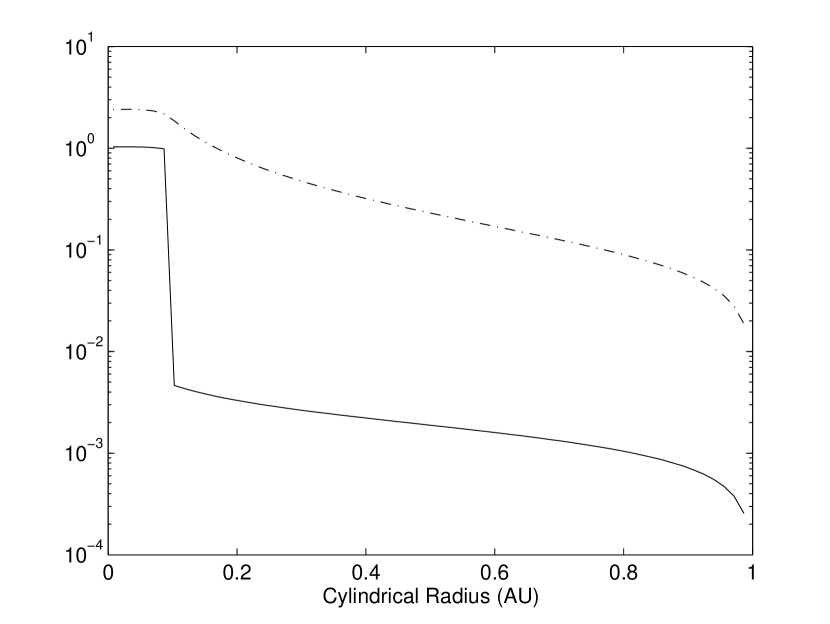
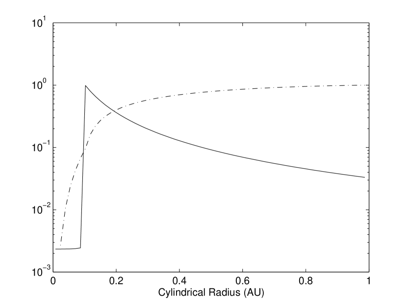
Figure 1: Launching conditions of the reference simulation. Plotted are the vertical component of the injection velocity in units of $200{\,{\textnormal{km}}\,{\textnormal{s}}^{-1}}$ (solid) and the vertical field strength in units of $20\,{\textnormal{G}}$ (dash-dot) in the upper panel, and the mass density at the base of the wind in units of $2\times 10^{-13}{\,{\textnormal{g}}\,{\textnormal{cm}}^{-3}}$ (solid) and the cumulative mass flux from each side of the disk in units of $10^{-8}{{\,{\textnormal{M}}_{\sun}}{\,\textnormal{yr}}^{-1}}$ (dash-dot) in the lower panel.

Figure 1 shows the prescribed launching conditions for our reference simulation. Note that the axial injection region within $\varpi_{g}=0.1{\,\textnormal{AU}}$ contains about 10% of the cumulative mass flux from the disk in our simulation. This fraction can be made smaller by reducing the injection density, but it would take longer for the wind to reach a steady state because of a more stringent Courant condition. KLB03 investigated the effects of the axial injection and concluded that the structure and dynamics of the magnetocentrifugal part of the wind remained largely unchanged for differing mass fluxes in the axial region. We confirmed this result with a new set of simulations.

Computationally, we have used a grid with 256 active zones in both the $\varpi$ and $z$ directions. On both axes the grid spacing is linear for $0\leq\varpi,z\leq 1.2{\,\textnormal{AU}}$ with 76 zones, and logarithmic for $1.2\leq\varpi,z\leq 100{\,\textnormal{AU}}$ with 180 zones. This arrangement allows us to extend our simulation to large distances from the origin while still retaining good resolution of the launching region.

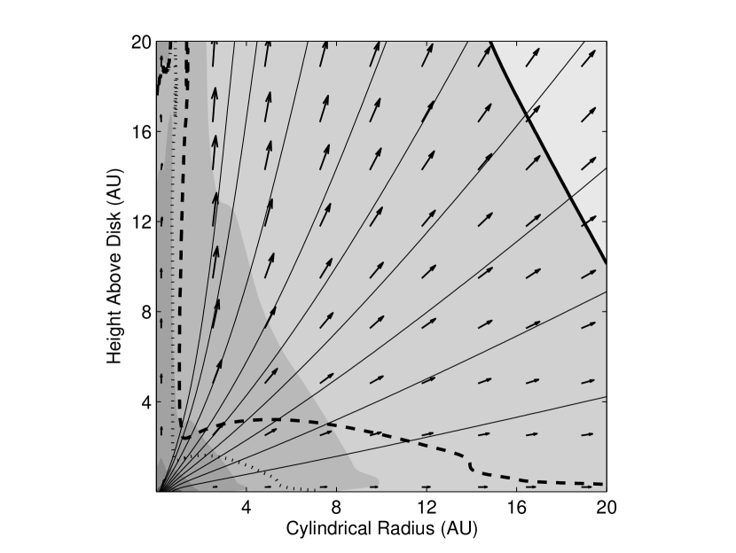
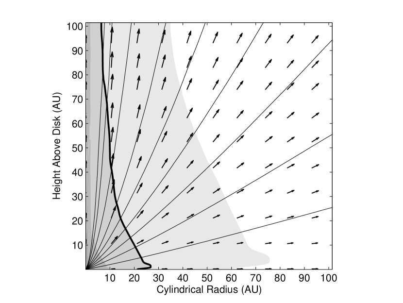
Figure 2: Steady-state wind solution in the reference simulation. Plotted as thin solid lines are the nine magnetic field lines that divide the wind into ten zones of equal mass flux. The velocity vectors are denoted by arrows, with the length of the arrow proportional to the poloidal flow speed. Density contours are shown in shades (one decade per shade), with the thick solid line marking $n_{H}=10^{4}{\,{\textnormal{cm}}^{-3}}$. The Alfvén and fast magnetosonic surfaces are shown in the top panel as a thick dotted line and thick dashed line respectively. The top panel shows the inner region of the simulation, while the lower one shows the full simulation box.

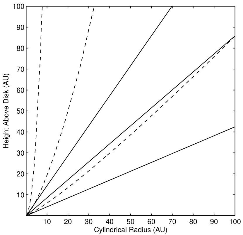
Figure 3: Comparison of initial to final magnetic field configuration for field lines enclosing 25%, 50%, and 75% of the total mass flux from the launching surface. The initial potential field is shown in solid lines, while the final, steady-state, field is shown in dashed lines.

The results of our reference simulation are shown in Figures 2–4. In Fig. 2, we plot the steady-state solution on two scales. On the smaller, $10{\,\textnormal{AU}}$ scale, we find that most of the space is filled with magnetocentrifugally accelerated wind material from the Keplerian part of the launching surface between $0.1$ and $1{\,\textnormal{AU}}$. The fast injection part of the wind, enclosed within the streamline closest to the axis, occupies a relatively small fraction of the space. The fraction decreases on the larger scale, as shown in the bottom panel. There is some residual nonsteadiness in the fast injection region, which has little effect on the magnetocentrifugal part of the wind. In both panels, gradual collimation is evident in both field line and density contour. The collimation appears more prominent in the axial region than in the equatorial region. Note the presence of bulging in density contours at low altitudes above the disk. The degree of bulging is related to the slope of the mass loading $\alpha_{m}$, as we show in § 3.3 (see also KLB03). It may affect the appearance of the axial jet.

Before discussing more quantitatively the acceleration and collimation of the reference wind solution, we note that its dimensionless mass loading parameter at the Keplerian part of the launching surface is given by

$$\mu(\varpi_{g}\leq\varpi\leq\varpi_{0})=\mu_{g}\left({\varpi\over\varpi_{g}}\right)^{2\alpha_{B}-\alpha_{m}-1/2}\left[{B_{z}(\varpi)\over B_{p}(\varpi){\cal S}(\varpi)}\right],$$ (17)

where the scaling constant

$$\mu_{g}\equiv{4\pi D_{0}\over B_{0}^{2}}\left({GM_{*}\over\varpi_{g}}\right)^{1/2}=6.25\times 10^{-3}$$ (18)

(where the density and field strength constants $B_{0}$ and $D_{0}$ are defined in equations [15] and [16]) and the exponent $2\alpha_{B}-\alpha_{m}-1/2=0$ for the reference run. The combination in the square bracket is not predetermined, since $B_{z}/B_{p}=\cos(\theta)$ and the angle $\theta$ between the poloidal field line and the disk normal is allowed to vary in response to the stresses in the wind. We find that in steady state the combination has values of order unity or less. Therefore, the reference wind has $\mu(\varpi)\ll 1$ on the launching surface. It is a “light” wind.

Even though the mass loading is relatively light, it causes significant flow collimation. This is shown in Fig. 3, where three representative field lines enclosing respectively 25, 50 and $75\%$ of the total mass flux are drawn. Also shown for comparison are the initial positions of these field lines, which correspond to the potential (current-free) field outside the launching surface; they mark where the field lines would be in the absence of the wind. Evidently, there is enough cross-field electric current flowing in the wind to substantially modify the initial potential field configuration, particularly at large distances, where the magnetic field is dominated by the toroidal component.

The flow collimation enables flux tubes to diverge faster than radial, causing the fast magnetosonic point to move from infinity to a finite radius (see the location of the fast surface in Fig. 2). Beyond the fast surface, flow acceleration continues, until most of the magnetic energy is converted into the kinetic form. The efficient conversion can be seen in the upper panel of Fig. 4, where the fast magnetosonic Mach number $M_{f}=\sqrt{4\pi\rho v_{p}^{2}/(B_{p}^{2}+B_{\phi}^{2})}$ is plotted as a function of spherical radius for the three selected field lines. The wiggles on the curve for the $25\%$ mass flux enclosing field line are caused by the nonsteady flow near the axis. At large distances away from the launching region, the ratio of kinetic to magnetic energy is approximately $M_{f}^{2}/2$ (Spruit, 1996). This ratio ranges from 2 to 3.1 at a radius of $100{\,\textnormal{AU}}$. They are much larger than the ratio of $\sim 0.5$ at $M_{f}=1$, pointing to significant acceleration of the wind plasma beyond the fast surface.

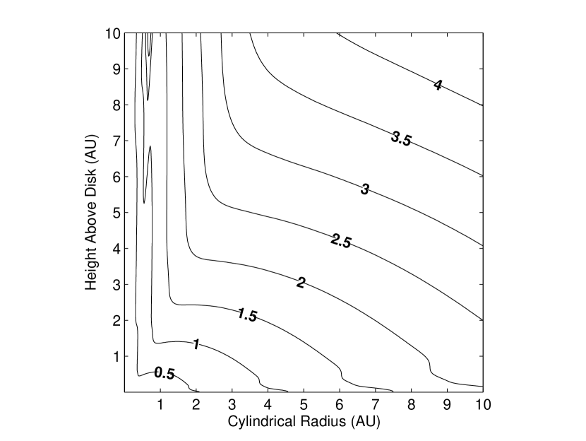
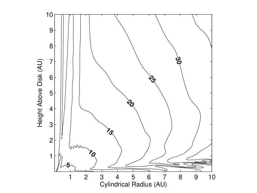
Figure 13: Contours of the ratio $|B_{\phi}|/B_{p}$ for the inner regions of the reference simulation with $\dot{m}_{0}=1$ (top panel) and the heavily loaded, $\dot{m}_{0}=1000$, simulation (bottom panel). Whereas the reference wind is initially dominated by the poloidal magnetic field, the heavily loaded wind is clearly dominated by the toroidal field all the way to the launching surface.

The lower panel of Fig. 4 displays the pitch angle $\theta_{B}=\tan^{-1}(|B_{\phi}|/B_{p})$ of the magnetic field along the three representative field lines. It shows clearly that the wind-launching field lines start out more or less straight (i.e., having small pitch angle), in accordance with the wind being relatively light. They become increasingly toroidal at large distances, especially beyond the Alfveń surface. The toroidal magnetic pressure gradient dominates the wind acceleration beyond the fast point (see also Fig. 13 below). Inside the fast point the centrifugal effect dominates. We now show that this basic behavior persists as long as the mass loading is lower than some critical amount.

3.2 Variation in Total Mass Loading

To explore the effects of mass loading on the wind structure, we have performed a series of simulations in which the only parameter that was varied from the reference run was the total amount of mass loading ${\dot{M}}_{w}$. We were able to obtain reliable solutions over a wide range of ${\dot{M}}_{w}$, from $0.1$ to $3000$ times the value for the reference solution, corresponding to $1\times 10^{-9}$ – $3\times 10^{-5}$ in units of $(B_{0}/19.2\,{\textnormal{G}})^{2}{{\,{\textnormal{M}}_{\sun}}{\,\textnormal{yr}}^{-1}}$. The mass loading used for each simulation (assuming the fiducial choice $B_{0}=19.2\,{\textnormal{G}}$), as well as some important data from the results, are summarized in Table 1. The second column shows the value of the characteristic mass loading parameter $\mu_{g}$ on the launching surface that is defined in equation (18). The quantities in the last three columns, $v_{\infty}$, $M_{f,\infty}$, and $\varpi_{j}$, are measured at a spherical radius of $100{\,\textnormal{AU}}$ along the 50% mass flux enclosing field line, which comes from the same location on the launching surface for all cases. As expected, the wind becomes slower and more collimated as the mass loading increases. Half of the mass flux is enclosed within $14{\,\textnormal{AU}}$ of the axis for the $3\times 10^{-5}{{\,{\textnormal{M}}_{\sun}}{\,\textnormal{yr}}^{-1}}$ wind, whereas the same fraction is enclosed within $48{\,\textnormal{AU}}$ in the $1\times 10^{-9}{{\,{\textnormal{M}}_{\sun}}{\,\textnormal{yr}}^{-1}}$ case.

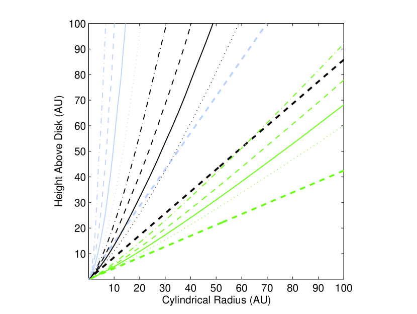
Figure 5: The 25% (blue), 50% (black), and 75% (green) mass flux enclosed field lines plotted for the simulations with $\dot{m}_{0}=0.1$ (dotted lines), $\dot{m}_{0}=1$ (reference solution, solid), $\dot{m}_{0}=10$ (dashed), and $\dot{m}_{0}=100$ (dash-dotted). The degree of magnetic field collimation clearly increases with mass load. Also plotted in thick dashed lines is the initial potential field.

To illustrate the wind collimation in more detail, we plot in Fig. 5 three field lines enclosing respectively $25$, $50$ and $75\%$ of the total mass flux for each of the four representative cases ${\dot{m}}_{0}=0.1$, $1$, $10$, and $100$, where ${\dot{m}}_{0}$ is the wind mass flux ${\dot{M}}_{w}$ scaled by $10^{-8}\times(B_{0}/19.2\,{\textnormal{G}})^{2}{{\,{\textnormal{M}}_{\sun}}{\,\textnormal{yr}}^{-1}}$; the ${\dot{m}}_{0}=1$ case thus corresponds to the reference run. The scaled mass flux is related to the characteristic mass loading parameter defined earlier by

$$\mu_{g}=6.25\times 10^{-3}{\dot{m}}_{0}.$$ (19)

Note that the lightest (${\dot{m}}_{0}=0.1$) wind is also the least collimated, as expected. Nevertheless, its field lines are still much better collimated than the initial potential configuration, despite the small dimensionless mass loading parameter at the launching surface: $\mu\sim 5\times 10^{-4}$. As ${\dot{m}}_{0}$ is lowered even further, the fast surface starts to extend beyond the computation box, making the simulation unreliable. Furthermore, the Courant condition becomes more stringent for the lower values of mass loading, setting a practical lower bound on ${\dot{m}}_{0}$ because of computer time constraints. In any case, judging from the spacing between the field lines of different mass loading in Fig. 5, it appears that a further reduction of ${\dot{m}}_{0}$ by at least several orders of magnitude would be needed for the field lines to approach the potential configuration. An implication is that the potential configuration can rarely, if ever, be a good approximation to the magnetic field struture of the (non-relativistic) magnetocentrifugal winds relevant for star formation, particularly at large distances; the structure must be determined numerically by solving the cross-field force balance equation.

3.2.1 Steady “Light” Winds

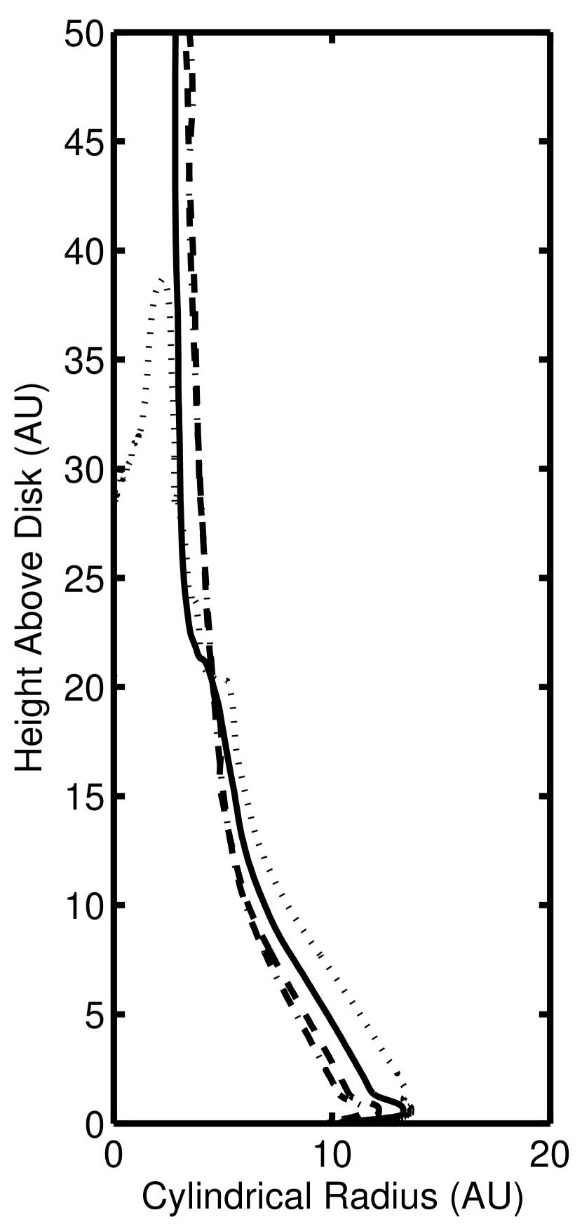
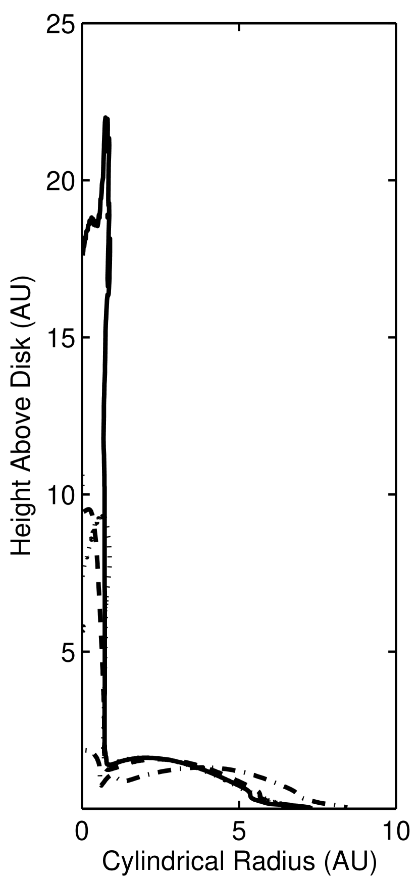
Figure 6: Plotted are the rescaled density contours (left panel) and the Alfvén surface (right panel) for solutions of different mass loading – the dotted line corresponds to $\dot{m}_{0}=0.1$, solid $\dot{m}_{0}=1$ (reference solution), dashed $\dot{m}_{0}=10$, and dash-dotted $\dot{m}_{0}=100$. The rough alignment in both panels demonstrates that the winds are approximately self-similar in some aspects.

Our wind solutions of different mass loading are approximately self-similar in several aspects. These include the isodensity contours and the Alfvén surface, which can be made to line up rather well through simple rescaling, as shown in Fig. 6. The left panel plots the contour of constant number density $5\times 10^{4}{\dot{m}}_{0}^{4/3}{\,{\textnormal{cm}}^{-3}}$. The contours of scaled density roughly align. In the right panel, we plot the Alfvén surface with both $z$ and $\varpi$ multiplied by ${\dot{m}}_{0}^{1/3}$. Again, most of the surfaces line up well, except for the heaviest wind shown. The deviation is an indication that the wind may behave differently at the high mass loading end. Interestingly, the position of the Alfvén surface in the simulations closely follows that predicted for purely radial winds (Spruit, 1996)

$$\frac{\varpi_{A}}{\varpi_{0}}=\left[\frac{3}{2}\left(1+\mu^{-2/3}\right)\right]^{1/2}$$ (20)

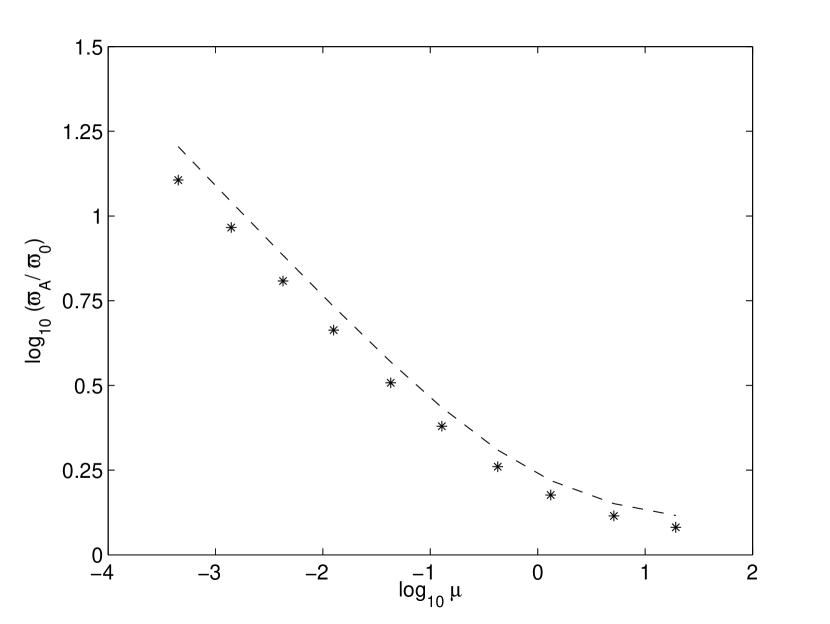
Figure 7: Log-log plot of the ratio of the cylindrical radius of the Alfvén point $\varpi_{A}$ to that of the footpoint $\varpi_{0}$ as a function of the mass loading parameter $\mu$ (at the footpoint) for the 50% streamline. The stars are values taken from our simulations while the dashed line shows the expected values based on equation (71) of Spruit 1996), which was derived for a radial wind geometry.

as shown in Fig. 7, which includes both “light” and “heavy” winds (with $\mu\raise 1.29167pt\hbox{$>$}\kern-7.5pt{\lower 2.79857pt\hbox{$\sim$}}1$, to be discussed below).

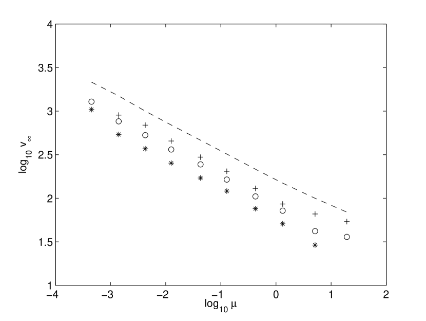
Figure 8: Log-log plot of the poloidal velocity of the wind along the 25 (+), 50 (o), and 75% (*) streamlines at a radius of $100{\,\textnormal{AU}}$ from the origin as a function of the mass loading. A power-law with index $-1/3$ is also displayed for comparison.

In Fig. 8, we plot the poloidal flow speed $v_{\infty}$ at a spherical radius of $10^{2}{\,\textnormal{AU}}$ for three representative field lines (enclosing respectively 25, 50, and 75% of the total mass flux) for a number of ${\dot{m}}_{0}$. The data points follow a power law distribution $v_{\infty}\propto{\dot{m}}_{0}^{-\alpha_{v}}$, with $\alpha_{v}\approx 1/3$. At the low ${\dot{m}}_{0}$ end, there is a slight deviation from power-law; this is most likely due to the fact that the fast surface approaches the outer edge of the simulation box, which leaves little room for the wind to accelerate beyond the fast surface to a terminal speed. There is also a deviation present at large values of ${\dot{m}}_{0}$ where the slope of the power appears to become more shallow. We note that the index of the power law distribution of terminal speed with respect to the mass loading is close to 1/3, as in the simplest case of radial wind geometry (see equation [2]). The agreement is all the more remarkable considering the fact that the fast point is no longer at infinity because of wind collimation, and that there is substantial increase in flow speed beyond the fast point, by a factor up to $\sqrt{3}$ for light winds. To be more quantitative, we note that at large distances from the launching region, the asymptotic speed along any field line can be written in a form

$$v_{\infty}=\left({\Omega^{2}M_{f}^{2}B_{p}\varpi^{2}\over 4\pi\kappa}\right)_{\infty}^{1/3}.$$ (21)

The relation is obtained from the definition of the fast Mach number, the conservation of mass-to-flux ratio (equation [7]), and the flux freezing condition (equation [8]). It is a generalization of equation (2) to an arbitrary poloidal field geometry. In the radial field limit, where $M_{f,\infty}=1$ and $B_{p}\varpi^{2}$ is constant along a field line, we have $v_{\infty}\propto\kappa^{-1/3}\propto\mu^{-1/3}$, recovering the scaling in equation (2). When the flow collimation is taken into account, neither $M_{f,\infty}=1$ nor constant $B_{p}\varpi^{2}$ holds along a field line. The fact that the scaling $v_{\infty}\propto{\dot{m}}_{0}^{-1/3}\propto\mu^{-1/3}$ still holds approximately implies that the combination $(M_{f}^{2}B_{p}\varpi^{2})_{\infty}$ varies little with mass loading. Apparently, the reduction of the (geometric) quantity $B_{p}\varpi^{2}$ due to the field collimation is more or less offset by the continued conversion of magnetic to kinetic energy beyond the fast point, which increases the Mach number $M_{f}$.

3.2.2 Heavily-Loaded Winds

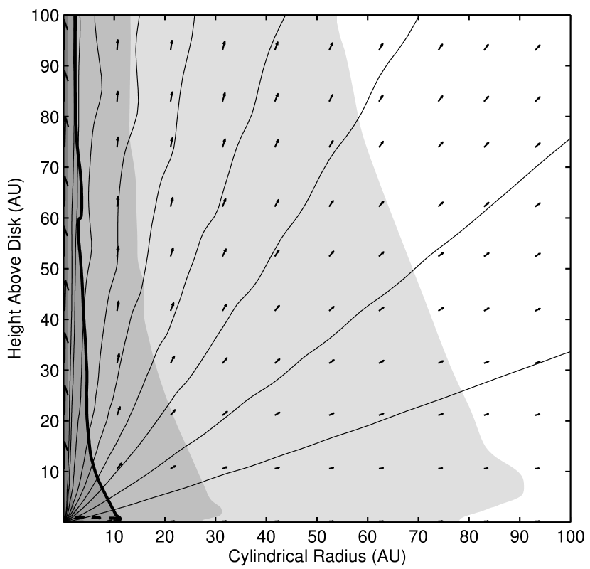
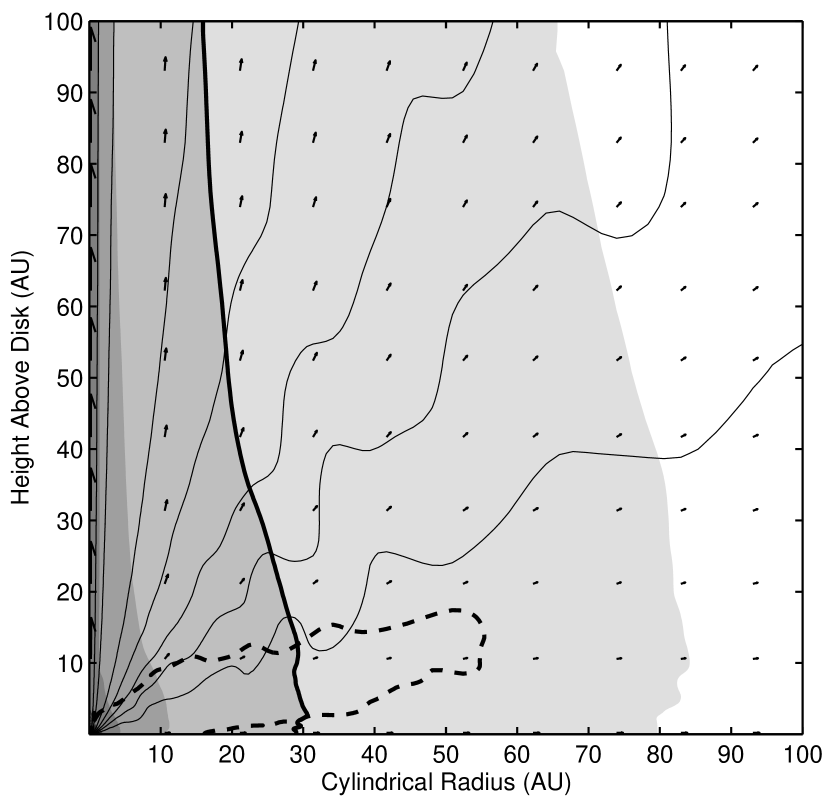
Figure 9: Wind solutions for the mass loading values of $\dot{m}_{0}=300$ (top panel) and $\dot{m}_{0}=3000$ (bottom panel), showing the nonsteady flow behavior in the “heavy” wind regime. The field lines are shown as thin, solid lines, the fast magnetosonic surface as a thick, dashed line, and the $10^{8}{\,{\textnormal{cm}}^{-3}}$ contour as a thick, solid line. Greyscale indicates number density (one decade per shade), and arrows show the direction and magnitude of the poloidal velocity field. Note that the amplitude of oscillation increases with mass loading.

Above some mass load, the wind solution remains perpetually unsteady. The inability to reach steady state begins around ${\dot{m}}_{0}=300$, when ripples of small amplitude start to propagate along some field lines from near the launching surface to large distances. As the mass loading increases, the amplitude of the field line oscillation grows. In the upper panel of Fig. 9, we show a snapshot of the wind with ${\dot{m}}_{0}=300$ (corresponding to a characteristic mass loading parameter of $\mu_{g}=1.9$), after the wind has settled into a state of finite-amplitude oscillation. The origin of the oscillation is unclear. We suspect that it is related to the large toroidal magnetic field for a heavily loaded wind, which dominates the poloidal component from large distances all the way to the base of the wind (see discussion in § 4.1 and Fig. 13 below). As the mass loading increases further, the amplitude of oscillation grows, and the wind starts to turn chaotic. This is illustrated in the lower panel of Fig. 9, where the mass loading parameter is set to ${\dot{m}}_{0}=3000$, and chaotic flow behavior is about to set in. For higher mass loading, we can trace the chaotic flow behavior to the generation of dense blobs near the launching surface, as the poloidal field lines bend inwards. The inward bending renders the centrifugal acceleration inoperative, as first pointed out in Krasnopolsky (2000). In practice, the inward bending of the poloidal field lines should also reduce the mass loading rate, which is fixed in the current simulation. We will return to this point in the discussion section.

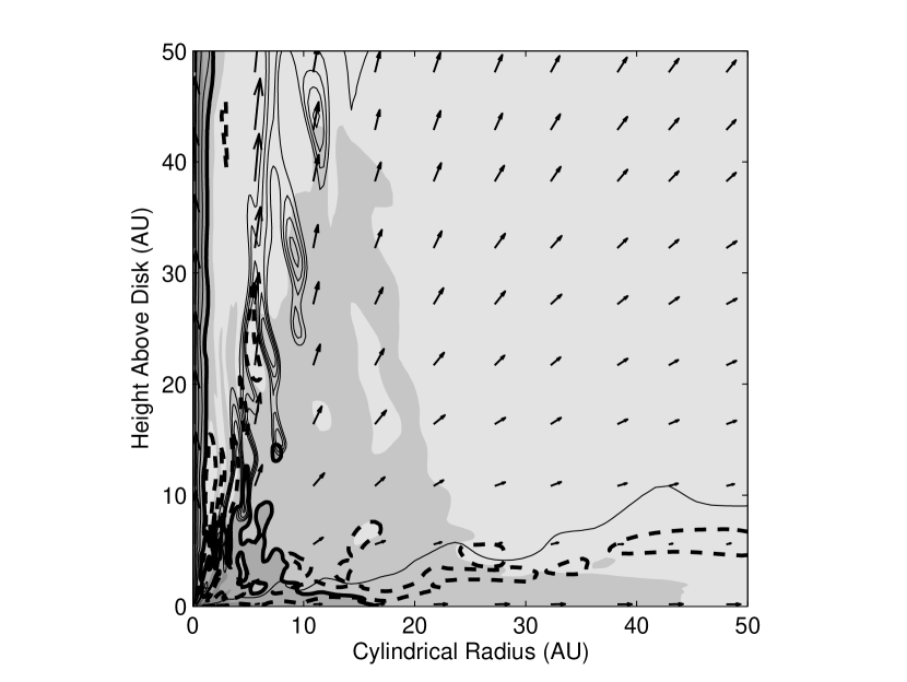
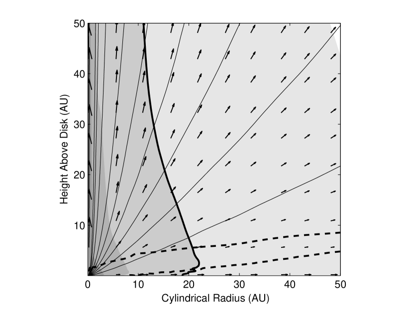
Figure 10: Wind solutions for mass loading value $\dot{m}_{0}=1000$ with initial injection speed $V_{o}=0.1$ (top panel) and $V_{o}=0.01$ (bottom panel). The field lines are shown as thin, solid lines, the fast magnetosonic surface as a thick, dashed line, and the $10^{8}{\,{\textnormal{cm}}^{-3}}$ contour as a thick, solid line. Greyscale indicates number density (one decade per shade), and arrows show the direction and magnitude of the poloidal velocity field.

We find that the level of nonsteadiness can be reduced by decreasing the initial wind injection speed, keeping the mass loading the same. We have also done a set of simulations using a larger initial injection speed ($V_{o}=0.1$ instead of 0.01, see equation [13] for definition of $V_{o}$). In these simulations the unsteady behavior set in for lower values of ${\dot{m}}_{0}$: oscillations appear at ${\dot{m}}_{0}=30$ and for ${\dot{m}}_{0}=1000$ the solution was completely chaotic. Figure 10 shows a comparison of the $\dot{m}_{0}=1000$ simulation using the different injection speeds. In the top panel we show the $V_{o}=0.1$ case which is completely chaotic. Upon reducing $V_{o}$ to $0.01$ we obtain a relatively steady solution (bottom panel) for this mass load. We believe the reduction of $v_{z}$ produces a cleaner result in the cold wind limit. How this result would be modified in the presence of a dynamically important thermal pressure near the base of the wind is a subject of future investigation.

3.3 Variation in the Distribution of Mass Loading

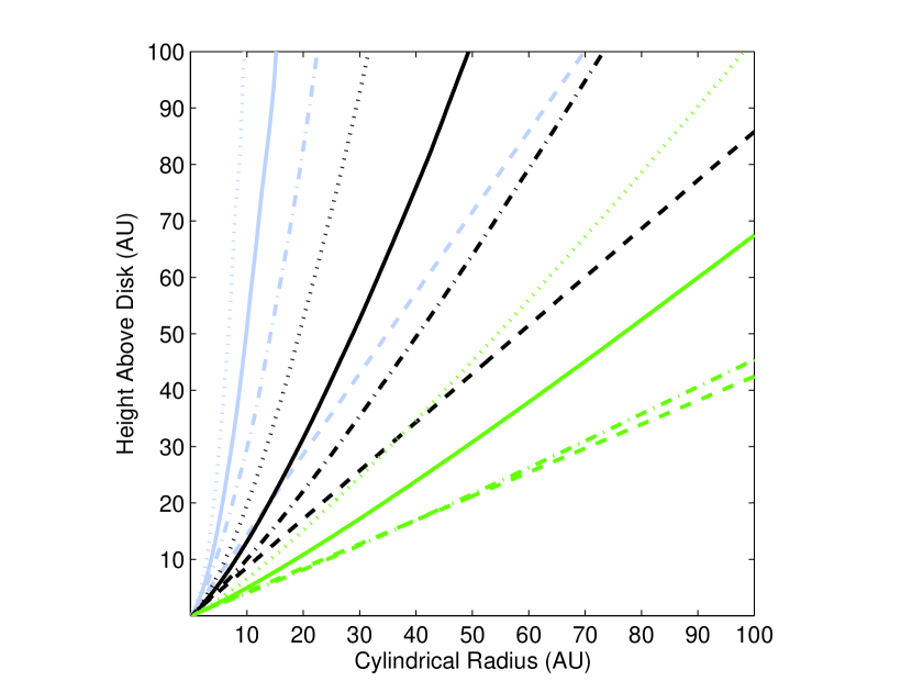
Figure 11: Three field lines plotted for simulations with same total mass flux, but differing mass loading distributions (25% line - blue, 50% line - black, 75% line - green). The dotted line corresponds to $\alpha_{m}=1$, solid $\alpha_{m}=2$ (reference solution), and dash-dotted $\alpha_{m}=3$. The thick dashed line shows the initial field for all three cases. The degree of magnetic field collimation clearly increases with decreasing $\alpha_{m}$. For the steep $\alpha_{m}=3$ mass loading, the mass load at the outer edge of the launching surface is so slight that it has hardly bent the field away from its initial configuration.

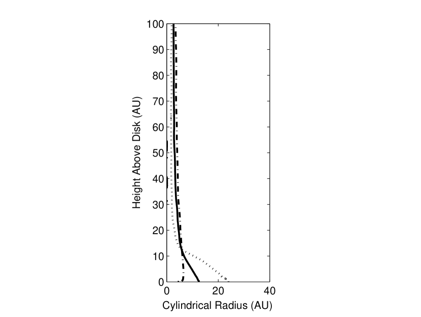
Figure 12: Density contours ($n_{H}=5\times 10^{4}{\,{\textnormal{cm}}^{-3}}$) for different mass loading distributions. The solid line corresponds to $\alpha_{m}=2.0$ (reference solution), the dotted line $\alpha_{m}=1.0$, and dash-dotted line $\alpha_{m}=3.0$. The solutions have all been scaled such that the total mass flux is $10^{-8}{{\,{\textnormal{M}}_{\sun}}{\,\textnormal{yr}}^{-1}}$.

The reference solution and its variants discussed in the last two subsections all have a dimensionless mass loading parameter $\mu$ more or less uniform across the surface of magnetocentrifugal wind launching. There is the possibility that the conclusions drawn may depend on this special feature of the solutions. To investigate whether this is the case, we have carried out several simulations in which $\mu$ varies substantially on the launching surface. The desired variation can in principle be obtained by changing either the magnetic flux distribution or the distribution of mass loading. We choose the latter, by varying the exponent $\alpha_{m}$ for the density distribution on the launching surface from 0.5 to 3, but fixing the total mass flux from each side of the disk to $\dot{M}_{w}=10^{-8}\times(B_{0}/19.2\,{\textnormal{G}})^{2}{{\,{\textnormal{M}}_{\sun}}{\,\textnormal{yr}}^{-1}}$. The results are shown in Figs. 11 and 12. Fig. 11 displays the steady state field configurations for three of the simulations. For each steady state solution, we plotted three field lines from the same three footpoints on the launching surface for all cases. The degree of collimation of field lines from a given footpoint is anticorrelated with the steepness of the mass loading slope, and, in fact, for the steepest simulation ($\alpha_{m}=3$) the last field line plotted is only barely collimated compared to the potential field configuration. The weak collimation is a result of small mass loading between that field line and the equatorial plane.

Density contours for the three simulations are shown in Fig. 12. Although the steepest mass loading simulation has the least collimated field from a given footpoint, it does possess the most “jetlike” density contours (i.e. the least amount of bulging at the base of the wind) — undoubtably due to most of the plasma being centrally concentrated on the launching surface. This solution is more attractive than the other two in explaining the nearly cylindrical appearance observed in some YSO jets, such as HH 30 (Burrows et al., 1996).

We have carried out a series of simulations for $\alpha_{m}=1$ and $\alpha_{m}=3$ where we have varied the total mass flux, keeping the distribution (i.e., $\alpha_{m}$) the same, as in § 3.2. We find that, as the mass loading increases, the shallower mass distribution simulations with $\alpha_{m}=1$ become unsteady sooner. The lower maximum load for steady winds in this case is probably a reflection of the fact that at large disk radii the rotation is slower and the field strength is smaller, both of which make the acceleration of a heavy load magnetocentrifugally difficult. Nevertheless, we have been able to verify that variations in mass loading still produce the same power law scalings in density contour and Alfvén surface locus for these alternate mass distributions as for the reference simulations. This indicates our results are not simply a fortuitous choice of mass distribution. Similarly the terminal velocities and magnetic lever arms follow the expected relations (see equations [18] and [19]).

4 DISCUSSION AND CONCLUSIONS

4.1 Mass Load Limit and Heavy Magnetocentrifugal Winds

A novel finding of our paper is that, for a given wind launching magnetic field, there exists a maximum mass load beyond which cold, steady state solution does not exist. For a relatively large wind injection speed of $10\%$ Keplerian, the maximum corresponds to a dimensionless parameter $\mu\sim 1$, which is roughly where the transition from “light” to “heavy” wind occurs. With the reduction of injection speed to $1\%$ Keplerian we can obtain rather steady solutions up to $\mu\sim 10$. The tendency for the solutions in the heavy wind regime to remain unsteady may not be too surprising, given that their magnetic fields are dominated by the toroidal component all the way to the launching surface. This is illustrated in Fig. 13 for the solution shown in lower panel of Fig. 10, where the mass loading is 1000 times higher than the reference solution. The toroidal field in the heavy wind is everywhere greater than the poloidal field in the magnetocentrifugal part of the wind. For comparison, the toroidal field in the light, reference solution starts to exceed the poloidal field only well beyond the launching surface. At the launching surface itself, the “heavy” wind has a ratio $|B_{\phi}|/B_{p}$ of 4, compared to a value of $0.2$ for the “light” wind. The toroidally dominated magnetic configurations are prone to pinch instability in lab experiments (Kruskal & Schwarzschild, 1954). A possible indication of the onset of this type of instability is the waviness of field lines in solutions with mass loads near but below the threshold for transition to chaotic flows (see Fig. 9). The fact that the threshold increases with decreasing injection speed at the launching surface points to another possibility for the nonsteadiness that involves the gravity of the central object — loss of mechanical balance near the launching surface for heavy winds.

The reason for the loss of balance can be seen from equation (8) for the conservation of angular velocity $\Omega$ along any field line in steady state. The equation can be cast into

$$v_{\phi}=\Omega\varpi+v_{p}B_{\phi}/B_{p}.$$ (22)

At the launching surface, the first term on the right hand side is set to the Keplerian speed in our simulations, and the second represents the speed that the wind fluid lags behind the Keplerian rotation (note that $B_{\phi}$ is negative). For a given injection speed $v_{p}$, the lag increases with the twisting of the field lines (i.e., the ratio of $|B_{\phi}|/B_{p}$), which in turn increases with mass loading. It is conceivable that beyond some threshold in mass load, the fluid rotation near the launching surface becomes too sub-Keplerian for the centrifugal force to balance the inward pull of the central gravity (Krasnopolsky, 2000). The force imbalance would lead to a radial infall of wind material, which is indeed observed in the initial phase of the development of chaotic flows, such as the one shown in upper panel of Fig. 10. The development of the chaotic behavior is reminiscent of that of the channel flows observed in simulations of weakly magnetized accretion disks (J. Hawley, priv. comm.). As one decreases the injection speed, the lag speed is decreased for a given magnetic field twist. This is consistent with our finding that decreasing the injection speed tends to make a heavy wind more steady. By choosing a small enough injection speed we were able to obtain more or less steady solutions well into the heavy wind regime, with $\mu\gg 1$. The fact that such heavy wind solutions can be obtained from time-dependent simulations suggests that they are stable to, or at least not disrupted by, axisymmetric (pinch) instabilities, despite their magnetic fields being completely dominated by the toroidal component. Whether they can resist disruption by non-axisymmetric (kink) instabilities in 3D remain to be determined.

Even for an arbitrarily small injection speed, we expect the wind solution to become chaotic beyond a certain mass load. The reason is still related to equation (8), which applies to both the launching surface and above. For a slowly injected wind, acceleration above the launching surface increases the poloidal speed, causing the fluid to rotate significantly below the rate needed for radial force balance when the magnetic field becomes toroidally dominated. Material fed into the wind starts to fall toward the central star, dragging magnetic field lines along with it. The inward bending of field lines further reduces the centrifugal acceleration and thus exacerbates the force imbalance, again reminiscent of the development of channel flows in weakly magnetized disks through magneto-rotational instability (Hawley & Balbus, 1991). This positive feedback can be cut off if the mass loading (which is fixed in our simulations) is allowed to vary in response to the field bending. The mass loading is expected to drop drastically when the (poloidal) field lines bend within roughly $30\arcdeg$ of the disk normal, the minimum angle for mass-loading by the magnetocentrifugal mechanism (Blandford & Payne 1982; Ogilvie & Livio 2001). The reduction is a natural way for the wind to self-limit its amount of mass loading. Quantifying this process requires a detailed treatment of the disk-wind coupling, which is beyond the scope of the present work (see, e.g., the early analytic work of Wardle & Königl 1993 and recent numerical simulations of Casse & Keppens 2002).

Ouyed & Pudritz (1999) addressed the issue of mass loading through numerical simulations. They found a transition from steady to non-steady wind solution as the mass load is decreased below some critical value; this trend is the opposite of the one we find. One possibility for the difference lies in the simulation setup at the launching surface. In their simulations, the toroidal field strength is prescribed at the disk surface, along with the magnetic flux distribution. This prescription essentially fixed the amount of energy (and angular momentum) flux extracted by the rotating magnetic fields from the disk proper (see the last term in the expression, equation [10], for the specific energy $E$). In general, these prescribed amounts cannot be carried away from the disk by the loaded wind material, as illustrated in Ouyed & Pudritz (1997a). They found a discontinuity in $B_{\phi}$ between the disk and the active zones in a test simulation with $B_{\phi}$ set to zero on the disk. The discontinuity indicates to us that the toroidal field near the base of the wind is trying to respond to stresses further out, while being constrained by a (formally) mismatched boundary condition. In our simulations, the toroidal field is allowed to adjust in response to the stresses in the wind both on the launching surface and in the active zones. We are able to obtain steady solutions for very low mass loads, limited only by the size of the simulation box (since the fast surface, which needs to be enclosed within the box to minimize boundary effects, increases in size as mass load decreases), and by computation time, because a lighter wind has a larger Alfvén speed, which requires a smaller timestep to simulate. Another possibility for the difference is that our magnetocentrifugal wind becomes super fast-magnetosonic within the computational box, whereas in their simulations a significant fraction of outflow remains sub-fast up to the outer boundary. One worry is that, in such sub-fast regions, signals can propagate from the outer boundary to the launching surface. In the numerical experiments of KLB99, the coupling between the outer boundary and launching surface appears capable of driving the magnetocentrifugal wind unsteady or even chaotic.

The non-steadiness in our high mass load winds has a different origin: it occurs when the field is in some sense too weak to accelerate the prescribed mass load steadily. In our interpretation, the maximum in mass loading has its root in the inability of a heavily loaded wind to find a stable cross-field force balance. Such a force-balance cannot be accounted for in 1D wind models along a prescribed flux tube. Even 2D (axisymmetric) models obtained by directly solving the steady wind equations, such as those of Sakurai (1987) and Najita & Shu (1994), fail to uncover this maximum. This is probably because the construction of steady wind solutions directly is difficult, and it has not been possible to explore a large parameter space as we did in this paper using the time-dependent simulations. One type of steady solutions for which parameter exploration is feasible is the self-similar solutions of Blandford & Payne (1982). However, the cross-field force balance of such solutions must be interpreted with care, because of singularities near the axis and at the infinity. For example, Sakurai (1987) pointed out that the “standard” solution of Blandford & Payne is less collimated than the potential magnetic field with the same flux distribution on the disk, as the result of a singular current density on the axis. Also, the self-similar solutions tend to recollimate at large distances, which is not observed in our non-self-similar steady solutions.

4.2 Scaling Laws for Magnetocentrifugal Winds

Self-collimation of streamlines is a basic feature of magnetocentrifugal winds. The general expectation is that, for a given distribution of magnetic flux, the wind becomes better collimated as the amount of mass loading increases (e.g., Pelletier & Pudritz 1992). This expectation is borne out by our solutions (see Fig. 4). The increase in the degree of collimation with mass load appears to be slow; fitting a power-law distribution to the cylindrical radius of a representative streamline (at a height of $100{\,\textnormal{AU}}$) listed in Table 1 as a function of mass load yields a rough relationship, $\varpi_{j}\propto{\dot{M}}_{w}^{0.1}$. This relationship does not apply to all streamlines. In particular, the first (on axis) and last (on equator) streamlines are the same for all of our winds (by design). The space-filling constraint tends to discourage rapid streamline collimation, particularly for winds launched from a region that is small compared to the computational domain. Nevertheless, it is difficult to predict the location of each individual streamline a priori. This needs to be determined through numerical computation.

A somewhat surprising result is that the wind speed along any given streamline scales with the mass load as ${\dot{M}}_{w}^{-1/3}$, originally derived for radial geometry, despite the fact that the streamline collimates to different degrees for different mass loads. A related result is that the Alfvén radius follows closely the analytical relation $\varpi_{A}(\mu)$ for a radial wind. Both results indicate that the energy and angular momentum extraction from the disk and the wind acceleration are insensitive to the relatively small differences in the degree of flow collimation for various mass loads. The fact that the appropriately scaled density contours and Alfvén surfaces closely align implies that magnetocentrifugal winds of different mass loads are approximately self-similar.

The distribution of mass loading also affects flow collimation. We have demonstrated that loading more material in the outer part of the wind tends to produce a better collimated streamline from a given location on the disk. This is probably due to a preferential increase in the toroidal field strength of the outer part, which enhances the cross-field gradient of the product $B_{\phi}\varpi$, which is largely responsible for flow collimation. On the other hand, concentrating more material near the inner edge of the Keplerian disk tends to produce better collimated density contours. The fact that jet-like density structure can be produced naturally, together with the detection of rotation signatures in T Tauri jets (Bacciotti et al. 2002; Coffey et al. 2004), lends strong support to the magnetocentrifugal model of jet formation (Shu et al. 1995; Anderson et al. 2003).

To summarize, we have numerically obtained axisymmetric magnetocentrifugal wind solutions for a wide range of mass loading for a given wind-launching field configuration. The range is limited from below by computation time, and from above by a form of instability that causes the wind to become chaotic. It testifies to the robustness of the magnetocentrifugal mechanism for outflow production. Whether the mass loading in actual astrophysical systems, such as YSO winds, covers as wide a range remains to be determined. It will probably be limited by the detailed physics of mass supply from the disk, and by the ability of the wind to withstand disruption by instabilities in 3D.

Table 1: Wind Parameters as a Function of Mass Load $\dot{M}_{w}$

$\dot{M}_{w}$ ($10^{-8}$ M☉ yr-1)	$\mu_{g}$	$v_{\infty}^{a}$ (km s-1)	$M_{f,\infty}^{a}$	$\varpi_{j}^{a}$ (AU)
3000.0	19.0	36	2.26	14
1000.0	6.3	42	2.43	19
300.0	1.9	72	2.83	26
100.0	0.63	105	2.78	30
30.0	0.19	164	2.92	30
10.0	6.3$\times 10^{-2}$	245	2.83	30
3.0	1.9$\times 10^{-2}$	363	2.70	32
1.0	6.3$\times 10^{-3}$	530	2.62	32
0.3	1.9$\times 10^{-3}$	763	2.47	36
0.1	6.3$\times 10^{-4}$	1285	2.28	48

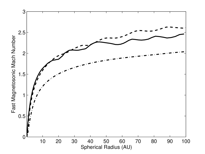
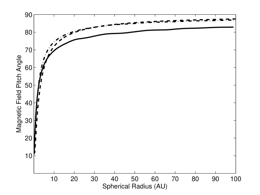
Figure 4: Reference simulation, showing the fast magnetosonic Mach number ${\cal M}_{f}$ (top panel) and the pitch angle $\theta=\tan^{-1}(|B_{\phi}|/B_{p})$ of magnetic field (bottom panel) as a function of spherical radius $r$ along three representative magnetic field lines. The solid line corresponds to the 25% mass flux enclosed field line, the dashed line the 50% line, and the dash-dot line the 75% line.

References

- Anderson et al. (2003) Anderson, J. M, Li, Z.-Y., Krasnopolsky, R. & Blandford, R. D. 2003, ApJ, 590, L107
- Bacciotti et al. (2002) Bacciotti, F., Ray, T. P., Mundt, R., Eislöffel, J., & Solf, J. 2002, ApJ, 576, 222
- Blandford & Payne (1982) Blandford, R. D., & Payne, D. G. 1982, MNRAS, 199, 883
- Bogovalov & Tsinganos (1999) Bogovalov, S., & Tsinganos, K. 1999, MNRAS, 305, 211
- Bontemps et al. (1996) Bontemps, S., Andre, P., Terebey, S. & Cabrit, S. 1996, A&A, 311, 858
- Burrows et al. (1996) Burrows, C. J., et al. 1996, ApJ, 473, 437
- Casse & Keppens (2002) Casse, F. & Keppens, R. 2002, ApJ, 581, 988
- Clarke, Norman, & Fiedler (1994) Clarke, D. A., Norman, M. L., & Fiedler, R. A. 1994, ZEUS-3D User Manual (Tech. Rep. 015; Urbana-Champaign: National Center for Supercomputing Applications)
- Coffey et al. (2004) Coffey, D., Bacciotti, F., Woitas, J., Ray, T. P., & Eislöffel, J. 2004, ApJ, 604, 758
- Contopoulos & Lovelace (1994) Contopoulos, J., & Lovelace, R. V. E. 1994, ApJ, 429, 139
- Edwards, Ray, & Mundt (1993) Edwards, S., Ray, T., & Mundt, R. 1993, in Protostars and Planets III, ed. E. H. Levy & M. S. Matthews (Tuscon: Univ. Arizona Press), 567
- Edwards et al. (1993) Edwards, S., et al. 1993, AJ, 106, 372
- Ferreira & Casse (2004) Ferreira, J. & Casse, F. 2004, ApJ, 601, L139
- Goldreich & Julian (1970) Goldreich, P. & Julian, W. H. 1970, ApJ, 160, 971
- Hardee & Rosen (2002) Hardee, P. E. & Rosen, A. 2002, ApJ, 576, 204
- Hayashi et al. (1996) Hayashi, M., Shibata, K. & Matsumoto, R. 1996, ApJ, 468, 37
- Hawley & Balbus (1991) Hawley, J. F. & Balbus, S. A. 1991, ApJ, 376, 223
- Heyvaerts & Norman (1989) Heyvaerts, J., & Norman, C. 1989, ApJ, 347, 1055
- Heyvaerts & Norman (2003) Heyvaerts, J., & Norman, C. 2003, ApJ, 596, 1270
- Königl & Pudritz (2000) Königl, A., & Pudritz, R. E. 2000, in Protostars and Planets IV, ed. V. Mannings, A. P. Boss, & S. S. Russell (Tuscon: Univ. Arizona Press), 759
- Krasnopolsky (2000) Krasnopolsky, R. 2000, PhD Thesis (Caltech)
- Krasnopolsky, Li, & Blandford (1999) Krasnopolsky, R., Li, Z.-Y., & Blandford, R. 1999, ApJ, 526, 631 (KLB99)
- Krasnopolsky, Li, & Blandford (2003) Krasnopolsky, R., Li, Z.-Y., & Blandford, R. 2003, ApJ, 595, 631 (KLB03)
- Kruskal & Schwarzschild (1954) Kruskal, M & Schwarzschild, M. 1954, Proc. R. Soc. London A, 223, 348
- Kudoh & Shibata (1995) Kudoh, T., & Shibata, K. 1995, ApJ, 452, L41
- Kudoh & Shibata (1997) Kudoh, T., & Shibata, K. 1997, ApJ, 474, 362
- Matsumoto et al. (1996) Matsumoto, R., Uchida, Y., Hirose, S., Shibata, K., Hayashi, M. R., Ferrari, A., Bodo, G., & Norman, C. 1996, ApJ, 461, 115
- Mestel (1968) Mestel, L. 1968, MNRAS, 138, 359
- Michel (1969) Michel, F. C. 1969, ApJ, 158, 727
- Najita & Shu (1994) Najita, J., & Shu, F. H. 1994, ApJ, 429, 808
- Ogilvie & Livio (2001) Ogilvie, G. I. & Livio, M. 2001, ApJ, 553, 158
- Okamoto (1999) Okamoto, I. 1999, MNRAS, 307, 253
- Ostriker (1997) Ostriker, E. C. 1997, ApJ, 486, 291
- Ouyed & Pudritz (1997a) Ouyed, R., & Pudritz, R. E. 1997, ApJ, 482, 712
- Ouyed & Pudritz (1997b) Ouyed, R., & Pudritz, R. E. 1997, ApJ, 484, 794
- Ouyed & Pudritz (1999) Ouyed, R., & Pudritz, R. E. 1999, MNRAS, 309, 233
- Pelletier & Pudritz (1992) Pelletier, G. & Pudritz, R. E. 1992, ApJ, 394, 117
- Pudritz & Norman (1986) Pudritz, R. E., & Norman, C. A. 1986, ApJ, 301, 571
- Romanova et al. (1997) Romanova, M. M., Ustyugova, G. V., Koldoba, A. V., Chechetkin, V. M., & Lovelace, R. V. E. 1997, ApJ, 482, 708
- Sakurai (1987) Sakurai, T. 1987, PASJ, 39, 821
- Shibata & Uchida (1986) Shibata, K., & Uchida, Y. 1986, PASJ, 38, 631
- Shu et al. (1994) Shu, F. H., Najita, J., Ostriker, E. C., & Wilkin, F. 1994, ApJ, 429, 781
- Shu et al. (1995) Shu, F. H., Najita, J., Ostriker, E. C., & Shang, H. 1995, ApJ, 455, L155
- Spruit (1996) Spruit, H. C. 1996, Evolutionary Processes in Binary Stars, NATO ASI Series C., 477, 249
- Stone & Norman (1994) Stone, J. M., & Norman, M. L. 1994, ApJ, 433, 746
- Trussoni, Tsinganos, & Sauty (1997) Trussoni, E., Tsinganos, K., & Sauty, C. 1997, A&A, 325, 1099
- Ustyugova et al. (1995) Ustyugova, G. V., Koldoba, A. V., Romanova, M. M., Chechetkin, V. M., & Lovelace, R. V. E. 1995, ApJ, 439, L39
- von Rekowski & Brandenburg (2004) von Rekowski, B. & Brandenburg, A. 2004, A&A, 420, 17
- Wardle & Königl (1993) Wardle, M., & Königl, A. 1993, ApJ, 410, 218