A 4.8- and 8.6-GHz Survey of the Large Magellanic Cloud: I The Images

Abstract

Detailed 4.8- and 8.6-GHz radio images of the entire Large Magellanic Cloud with half-power beamwidths of 33$\arcsec$ at 4.8 GHz and 20$\arcsec$ at 8.6 GHz have been obtained using the Australia Telescope Compact Array. A total of 7085 mosaic positions were used to cover an area of 6^∘ on a side. Full polarimetric observations were made. These images have sufficient spatial resolution ($\sim$8 and 5 pc, respectively) and sensitivity (3 $\sigma$ of 1 mJy beam^-1) to identify most of the individual SNRs and H II regions and also, in combination with available data from the Parkes 64-m telescope, the structure of the smooth emission in that galaxy. In addition, limited data using the sixth antenna at 4.5 to 6-km baselines are available to distinguish bright point sources ($<$ 3 and 2 arcsec, respectively) and to help estimate sizes of individual sources smaller than the resolution of the full survey. The resultant database will be valuable for statistical studies and comparisons with x-ray, optical and infrared surveys of the LMC with similar resolution.

1 INTRODUCTION

The Large Magellanic Cloud (LMC) is an excellent laboratory for investigation of the processes of star birth and death, and particularly the interactions of the stellar population and various components of the interstellar medium (ISM). To measure many properties of the sources, such as luminosity and physical size, we must know their distances. This is hard to do for objects in the Milky Way because most of the measured quantites are themselves dependent on the distance and there is also obscuring material within the Milky Way itself which can blank our view and distort optical measurements. In the LMC all sources of emission are at essentially the same known distance of 50 kpc.

Radio continuum observations can be used to measure both thermal emission from H II regions and polarized synchrotron emission from supernova remnants (SNRs). The thermal emission has a nearly flat radio spectrum whereas the synchrotron emission, from relativistic electrons accelerated in shocks and the magnetic fields of SNRs, has a power-law spectrum with brighter emission at lower frequencies. Three important sources of stellar energy in the ISM are UV radiation, fast stellar winds, and supernovae. Thus the radio observations supply a vital component in studies of these energy sources, by tracing the contributions from the photoionized and shock-ionized material and (through polarimetry) showing the orientation of magnetic field lines, even deep within highly obscured regions like molecular clouds. In combination with optical line emission (Smith, 1999) and X-ray images (Snowden, 1999) from the new generation surveys at those wavelengths, high-resolution radio continuum imaging will help to construct a complete physical picture of stellar feedback in the Magellanic Clouds.

We have completed 4.8- and 8.6-GHz observations of the LMC to produce images $6^{\circ}$ on a side, including all the bright features in that galaxy. They have resolutions of 33″ at 4.8 GHz (20″ at 8.6 GHz) or about 8 pc (5 pc) at the 50 kpc distance of the LMC. With these moderate-resolution data in hand, one can choose smaller areas for followup imaging, and reuse these relatively short-spacing data.

The noise level of the system provides 3-$\sigma$ measurements at 1 mJy beam^-1 and if the source fills the 33$\arcsec$ beam at 4.8 GHz, this value corresponds to a surface brightness at of 4$\times$10^-22 W m^-2 Hz^-1 sr^-1 or for a mean SNR spectral index of $-0.5$, a 1 GHz surface brightness of 1$\times$10^-21 W m^-2 Hz^-1sr^-1. While this limit is ten times the brightness of the faintest SNR in the Milky Way (G182.4+4.3, Kothes et al. (1998)) it would include 90% of all the Milky Way SNRs cataloged by Green (http://www.mrao.cam.ac.uk/surveys/snrs/).

2 OBSERVATIONS

2.1 Telescope Configurations

The observations were made simultaneously at 4.80 and 8.64 GHz using the Australia Telescope Compact Array (ATCA) consisting of five moveable 22-meter antennas and a sixth one fixed at a distance of 3 km from the end of the 3-km track available for the moveable antennas (Australia Telescope, 1992). For this program, two configurations of the inner five antennas were used – 367 and 352 meters. Together they provided nineteen antenna spacings between 31 and 367 meters separated by 15.3 meters with four gaps of 30.6 meters. This setup gave nearly complete coverage of the available spacings and thus a well sampled beam. The surface brightness of the dominant H II region, molecular cloud complex 30 Doradus is over 1.3 Jy beam^-1 at 4.8 GHz, the SNR N132D is over 0.4 Jy beam^-1 and several other sources approach that value. The desire to detect sources as faint as 1 mJY beam^-1 thus necessitated a dynamic range of over 1000/1. Extending the spacings of the antennas to improve the resolution would have resulted in sparser sampling of the spatial frequency plane ($uv$-plane) with increased sidelobe levels and a lower dynamic range. The declination of the LMC is close enough to the south pole that the beam for this east-west array is nearly circular.

The complex southeastern quarter of the galaxy was observed with an additional 375-meter configuration. This added three additional spacings to improve the beam pattern somewhat and also increased the sensitivity in that area by $\sqrt{3/2}$.

Data from the sixth antenna were also recorded to give a set of longer spacings reaching resolutions of 3″ at 4.8 GHz and 2″ at 8.6 GHz. Without intermediate spacings, it is not possible to construct a proper beam at this resolution but correlation of the data from antenna 6 with the others can be used to compare the flux density of a given source with that determined from the more complete synthesis with lower resolution to see what fraction of the source is unresolved on the complete image at the lower resolution. This procedure helps in the identification of background sources seen through the LMC. Full images with the higher resolution data have not been constructed but readers may obtain the data for any given position and make the images themselves.

The nominal bandwidth of the system at each frequency is 128 MHz split into thirty-two 4 MHz channels. No narrow band interference was detected in the individual channels. To account for edge effects in the filters, the inner 104 MHz was used at each band.

2.2 Observing Procedure

The observations were carried out during five extended runs with the ATCA. The 375-configuration was observed in March 2001; the 367-configuration in March 2002 and December 2002; and the 352-configuration in December 2001 and March 2003. The total observing time for this project was 496 hours.

The final image encompasses an area 6^∘ on a side centered at $05^{h}19^{m}00^{s}$ and $-69^{\circ}00\arcmin 00\arcsec$ (J2000). It includes almost all of the important objects in the LMC. To cover an area that large, a mosaic of images at 7085 individual pointing positions was made. This number included a few makeups for mis-pointings, increased coverage particularly toward 30 Dor, etc. The pointings were arranged in a so-called “hexagonal pattern” of equilateral triangles such that each point was equidistant from six surrounding ones. With circular symmetry in the beam this arrangement allows a slightly larger spacing between points than the normal 1/2 HPBW for a standard rectangular pattern. The adopted separation between points was $5\farcm 0$. This distance was a compromise that somewhat oversampled at 4.8 GHz (HPBW $9\farcm 8$) and somewhat undersampled at 8.6 GHz ($5\farcm 4$).

The entire area was broken into 16 tiles, each $1.5^{\circ}$ on a side. Each tile was observed during a full 12-hour observing “day” in each configuration. There were four fields within one tile and two observing patterns within a field to minimize move time and provide as much hour angle coverage per pointing as practical. The observing patterns were laid out as shown in Figure 1 with 9 colums of 6 vertical points alternating with 9 columns of 5 points each. Each point was observed for two 10 – 12 second integrations (depending on whether the observing “day” was 12 or 13 hours long plus compensation for any lost time) before moving to the next point in the pattern. The eight patterns for a given tile were staggered throughout an $\sim$ 3-hour period so that adjacent columns were observed at hour angles separated by $\sim$ 1 1/2 hours. The full 3-hour sequence of patterns, including calibration observations, was cycled four times to give eight reasonably uniformly spaced hour angles for each location in the galaxy. The total integration time per pointing was thus $\geq 8\times 20^{s}$.

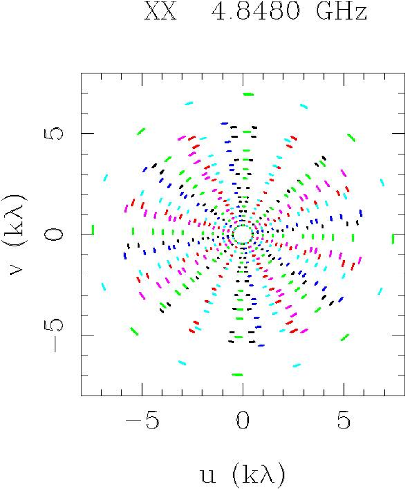
Figure 2: Coverage of the spatial frequency ($uv$) plane at 4.8 GHz for both patterns covering one field with all arrays. Note that this covers only the inner 400 meters and does not include the data fron the distant 6-km antenna.

The observations with the second telescope configuration were obtained at hour angles that interleaved with those from the first configuration, double the final number of hour angles. Figure 2 is a plot of the $uv$ coverage of the field including the bright H II region complex 30 Dor (Bode, 1801) which included all three array configurations. Each short arc is the coverage for one baseline for the duration of one observing pattern.

The individual fields and tiles were positioned such that the pointing separations were maintained over the tile boundaries. Because the right ascension separations are measured in hours of right ascension rather than angular distance on the sky, the right ascension separation varies with declination. In practice, the separation was held constant in right ascension for each field and set to be correct for the northern most points in the field so that the separations were always the designated 5$\arcmin$ or slightly less.

Absolute calibration was obtained by observations of PKS B1934-638 for which flux densities of 5.8 and 2.8 Jy at 4.8 and 8.6 GHz, respectively, were adopted from the memo by Reynolds (http://www.atnf.csiro.au/observers/memos/d96783~1.pdf). PKS B0454-810 was used for phase and pointing calibration.

3 DATA REDUCTION

3.1 Total Intensity

The data were split into the two frequency bands, edited and calibrated using standard MIRIAD (Sault, Teuben, and Wright, 1995) routines. To compromise between the desire for full sensitivity from natural weighting of the data and high resolution with a good beam pattern from uniform weighting, a Briggs’ (1995) robust weighting of 0 was adopted. The resultant half-power beamwidths were 33″ at 4.8 GHz and 20″ at 8.6 GHz.

Because the baseline lengths are all multiples of 15 meters, there is a bright grating ring with a radius of 14$\farcm$3 at 4.8 GHz (and 8$\farcm$0 at 8.6 GHz) around all strong sources. To remove this ring by the CLEAN process it is necessary to construct images large enough to encompass this ring which lies well outside the primary beam of the individual antennas. Thus the usual mosaic mode of imaging in MIRIAD could not be used. Instead, each pointing was imaged, CLEANed and restored individually before combining into the final mosaic of the entire galaxy. The individual images were 500 8″ pixels on a side at 4.80 GHz and 500 5″ pixels at 8.6 GHz.

To assess the noise level on the final image, statistics were determined for six different randomly-placed boxes with areas of about 900 square arcmin containing no sources brighter than 5 mJy beam^-1. The average rms noise was 0.28 mJy beam^-1 at 4.8 GHz and 0.50 mJy beam^-1 at 8.6 GHz. Because of the overlapping mosaic positions, the effective integration time at any location is roughly four times the value of $\sim 160$ sec per pointing position. Indeed the measured noise levels are close to the theoretical values of 0.31 mJy beam^-1 and 0.38 mJy beam^-1 at 4.8 and 8.6 GHz, respectively for continuum observations with the chosen arrays and an integration time of 640 sec (see http://www.atnf.csiro.au/observers/docs/at_sens/). In the southeastern quadrant where the third array was used, the rms noise levels were somewhat better at 0.25 and 0.46 mJy beam^-1, respectively. This is not quite as much gain as expected purely on the basis of observing time because of the significant confusion in this complex part of the LMC.

For the first pass of cleaning the images for each pointing we chose a cutoff brightness of 0.5 mJy beam^-1. Fewer than 10% of the positions did not converge at that level; in these cases a higher cutoff was adopted. All but about fifty positions converged at levels less than 0.7 mJy beam^-1. The others were in complex regions of bright sources and the dynamic range remained greater than 500/1.

The region around 30 Dor contains bright, complex emission which produces strong sidelobe structures. To improve the dynamic range there, we utilized archival ATCA data sets (Lazendic et al., 2000, 2003) which have near-complete $uv$-plane coverage for 30 Dor and N 157B, at both frequencies. We also included some makeup observations in the region of N 160 with more complete hour angle coverage than the survey observations.

3.2 Polarization

Stokes Q, U, and V images were constructed, cleaned, and mosaiced in the same manner as the total intensity ones. Because the square root of the sum of the squares of the Q and U stokes intensities will always be positive, the resultant polarized intensity images were statistically corrected for the Ricean bias to account for noise allowing negative intensities (Killeen et al., 1986; Vinokur, 1965). The Stokes V images, representing circular polarization show no structure above the noise level at either frequency. In general the linearly polarized intensities show no cross-polarization leakage above 0.1 mJy beam^-1 except toward the bright thermal source 30 Dor where the polarized intensities reach 2 mJy beam^-1 and 3 mJy beam^-1 to give leakages of 0.15% and 0.2% at 4.8 and 8.6 GHz, respectively.

The typical Faraday rotation for objects in the LMC is less than few hundred rad m^-2 (e.g., Dickel and Milne, 1995, 1998) so the total rotation across the band at 4.8 GHz would be less than 10^∘. We have thus ignored bandwidth smearing in the polarization data.

3.3 Addition of Parkes Data

As shown by Haynes et al. (1991), the LMC presents a complex field full of extended emission. Any interferometric observation aimed at studying the extended sources in the LMC will thus benefit from a database of complete short-spacing $uv$ coverage. The closest spacing between individual ATCA antennas of 30 meters cuts off those shortest available interferometer spacings. To include this information, we have utilized observations from the Parkes 64-meter telescope at 4.75 GHz and 8.55 GHz by Haynes et al. (1991). Both total intensity and polarization images were merged at 4.8 GHz but only the total intensity at 8.6 GHz because of the lack of sufficient polarized intensity to produce Parkes images at that frequency.

The ATCA data were directly observed in J2000 coordinates with a North Celestial Pole projection so the Parkes images were precessed, reprojected, and regridded to the same pixel size as the ATCA images. The images from the two telescopes were then combined with the MIRIAD routine IMMERGE which Fourier transforms both images to obtain their spatial frequency components, compares them in the region of overlap, and then creates the merged image by transforming the combined data sets.

After the precession, reprojection, and regridding, we also found that small translations of the Parkes images were needed to get the best alignment with the ATCA ones. The 4.75 GHz image was shifted 8″ east and 3″ north; the 8.55 GHz one was shifted 36″ east and 13″ north.

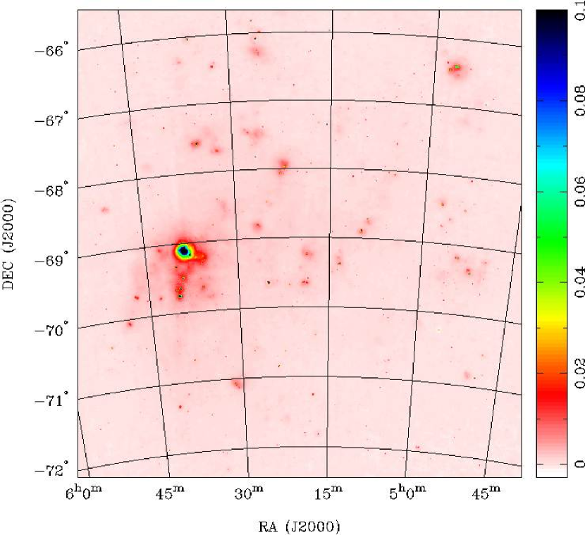
Figure 3: Full image of the Large Magellanic Cloud at a frequency of 4.8 GHz with a half-power beamwidth of 33 arcsec. The units on the wedge are Jy beam^-1.

To compare the integrated flux densities, we have summed them over the entire field of view shown in Figure 3 at 4.8 GHz but at 8.6 GHz the areas have been truncated to match the smaller area covered by the Parkes image at that frequency. The integrated flux density on the Parkes image is 305.4 Jy and, as expected, it is the same for the combined image. The ATCA image alone has an integrated value of 32.4 Jy or about 11% of the total. This number is consistent with the conclusion of Haynes et al. (1991) that about 40% of the emission from the LMC comes from discrete sources because several of the large H II region complexes, in particular 30 Doradus and N 11 in the northeast, cover areas of about 1/2^∘, much larger than the response size of the compact Array. At 8.6 GHz, the Parkes value is 321.4 Jy and the merged image gives 325.7 Jy, acceptably close. The integrated flux density from the ATCA is 18.8 Jy. or 6% of the total. We conclude that a significant fraction of the brightness of the LMC resides in features with scale sizes of order 10 arcmin, intermediate between the largest measurable sizes of the Compact Array at 8.6 GHz and 4.8 GHz.

The merging process is not perfect. Particularly at 8.6 GHz, there is some residual striping from the Parkes scanning pattern. More importantly, particularly around a few bright sources with diameters of about 2′, it can be seen that they appear to lie in a ring with a small bowl in the center corresponding to the 30-meter spacing. This structure is most obvious toward N 132D, the brightest radio SNR in the LMC, at $05^{h}25^{m}05^{s}$ and $-69^{\circ}37^{\prime}45^{\prime\prime}$. Because of the intermediate size of these sources, there is insufficient power in the adjacent parts of the spatial frequency plane in the Parkes data to fully compensate for this pattern in the synthesized image.

The normalization between the flux density scales for the Parkes observations in 1987-88 and the ATCA ones in 2001-03 was checked in two ways. The first was to compare the adopted flux densities for the source PKS 1934$-$638 after corrections for the slight differences in frequency. This comparison gave multiplying factors of 0.91 at 4.8 GHz and 1.09 at 8.6 GHz. The second method was to use the procedure in IMMERGE that determines the average ratio of the visiblilites in the overlap region between the ATCA and the Parkes telescope which was chosen to be 25 – 40 meters. This operation gave values of 0.88 at 4.8 GHz and 1.27 at 8.6 GHz. At 4.8 GHz, the two values were very close and a multiplier of 0.9 was adopted. To further evaluate the significant discrepancy between the values at 8.6 GHz, we attempted to minimize the bowl around N132D by trial and error. This resulted in a multiplier of 1.10, essentially the same as the ratio of the official flux density scales and so was adopted. We suggest that the average 8.6 GHz intensities are weak enough to be easily distorted by noise which produced a somewhat inaccurate ratio in the small region of overlapping visibilities sampled by IMMERGE.

4 RESULTS

4.1 Images

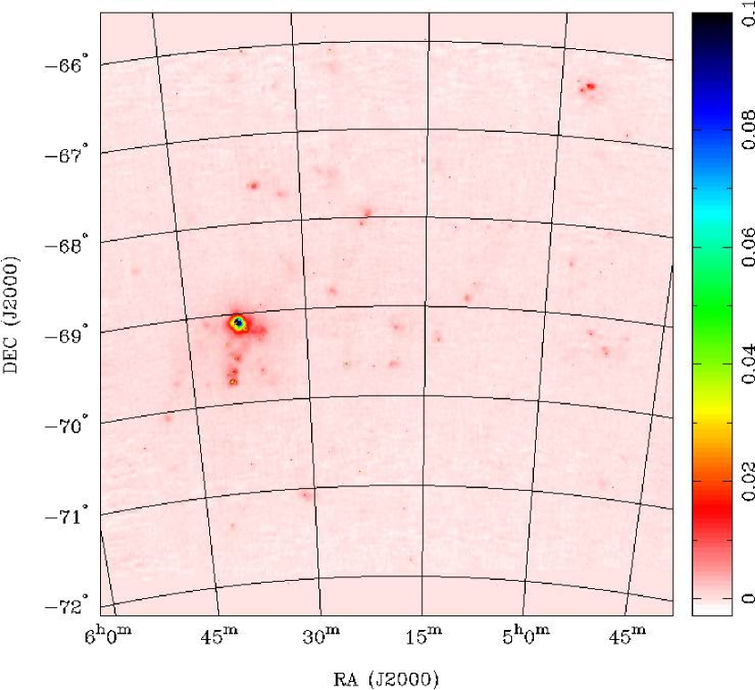
Figure 4: Fullimage of the Large Magellanic Cloud at a frequency of 8.6 GHz with a half-power beamwidth of 20 arcsec. The units on the wedge are Jy beam^-1.

The full merged images containing the data from the ATCA and Parkes are shown in Figures 3 and 4. The full dynamic range at 4.8 GHz covers surface brightnesses from about 0.0005 Jy beam^-1 to the peak of 30 Doradus at 1.3 Jy beam^-1 and so the color scale is a compromise to show as many interesting features as possible. Contours become too crowded to show details any better. The smaller beamwidth at 8.6 GHz reduces the surface brightness for a uniform source to 0.37 times that at 4.8 GHz so the color scale has been adjusted accordingly. H II regions should appear similar at both frequencies but supernova remnants and background sources are relatively fainter at 8.6 GHz. Sometimes the ripples that show up in the 8.6-GHz image in multiples of the $1\farcm 2$ scan increment make it difficult to see the relative brightnesses of the weak sources at the two wavelengths.

We have produced polarizarion images as well (see the data availability below) but do not show them here as virtually all the polarized emission bright enough to see is in fine scale features which are lost in the full-sized images. As noted by Haynes et al. (1991) even the Parkes data had to be smoothed to show detectable extended polarized structure. The polarization data from Parkes are included in the images at 4.8 GHz but have little effect.

In addition, to allow direct comparison, we have constructed images that have filtered the long spacings at 8.6 GHz and the short ones at 4.8 GHz to give the same range of spatial frequency response. This match filtering in the $uv$-plane is particularly useful when determining spectral indices for extended sources. At 8.6 GHz, this filtering is equibvalent to truncation of the $uv$ data at 8 k$\lambda$. We shall hereafter refer to these images as “match filtered” or “match truncated.” When merging with the Parkes data to get the full range of short spacings the filtering of the 4.8 GHz data is unnecessary. In practice the difference between the filtered and simply convolved total intensity images at 8.6 GHz was negligible so for the polarization images we have simply used the convolved Stokes Q and U images.

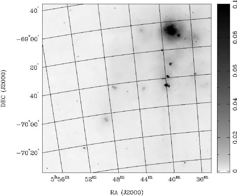
Figure 5: A detailed figure showing the 4800 MHz emission from the region around 30 Doradus. The units on the wedge are Jy beam^-1. The field of view is 1/16 of the total LMC mosaic. Figures 5a-p show detailed subregions across the entire LMC but are presented in the electronic edition only. Central coordinates for each subregion are given in Table 1.

Subimages are, of course, needed to see details of any area. We show sample images at 4.8- and 8.6 GHz of the area including the giant HII region - molecular cloud complex 30 Doradus in Figs. 5 and 6, respectively. The electronic version of the figures includes 16 total-intensity subimages at each frequency with 1450 pixels on a side and a 300 pixel overlap for each image. The central coordinates of these sub-images are listed in Table 1. They all have the same NCP projection and reference position at $05^{h}19^{m}00^{s}$ and $-69^{\circ}00^{\prime}00^{\prime\prime}$.

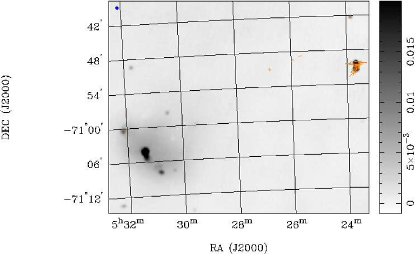
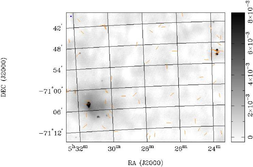
Figure 7: Images of the region containing the H II region and SNR complex N206 plus two small diameter sources. The greyscale is the total intensity with the units on the wedge in Jy beam^-1. The lines are the polarized electric vectors. The beam is shown in the upper left corner. a) 4.8 GHz where the longest vector represents a polarized intensity of 8 mJy beam^-1. b) 8.6 GHz where the longest vector is 4 mJy beam^-1 .

To illustrate the details that can be determined from more specific subimages showing every pixel, we show results on two sample areas. Figures 7 a,b are total intensity images at both frequencies with polarization e-vectors superposed of an area containing the H II region/SNR complex N206 on the east side at about $05^{h}31^{m}$ and $-71^{\circ}05^{\prime}$ and an apparent double source on the west side at $05^{h}23^{m}41^{s}$ and $-70^{\circ}51^{\prime}23^{\prime\prime}$. These and all subsequent images shown, both total intensity and polarization, are merged ATCA plus Parkes images. The polarized intensities are all truncated at 4 $\sigma$ so that most of the remaining vectors are real. The SNR is on the northeast side of N206 and is more prominant in the 4.8-GHz image than in the 8.6-GHz one because of its non-thermal spectrum. Although the polarimetric data are somewhat noisy at 8.6 GHz, we can see that the brightest part of the SNR is polarized whereas the larger H II region has only random vectors at about the 3-$\sigma$ level on the 8.6 GHz image. The SNR has already been investigated in more detail by Klinger et al. (2002).

The two small diameter objects on the western edge of Fig. 6 can just be discerned in the full images in Figures 3 and 4. They have been reported as a single source in all previous catalogs (e.g. Filipovic et al. 1995). They are both significantly polarized at each frequency and assuming no 180^∘ ambiguity (1163 rad m^-2) between the two frequencies, we determine mean Faraday rotations of +71 rad m^-2 for the northern source and $-$26 rad m^-2 for the southern one. These small values are typical of those found for the LMC in general (Klein et al., 1993).

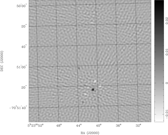
Figure 8: High resolution image at 4.8 GHz of the two small diameter sources in Figure 7. It is constructed from data taken only with the 6-km antenna correlated with each of the others so that it is sensitive only to features with a size of $<$ 3 arcsec. The units on the wedge are Jy (3-arcsec beam)^-1. This shows that the southern source is point-like while the missing northern one that should be at $05^{h}23^{m}41^{s}$ and $-70^{\circ}50^{\prime}18^{\prime\prime}$ is resolved out showing that it is extended.

Neither source significantly broadens the 20″ beam at 8.6 GHz, and because of the weak source intensity in the presence of the noise, it is not possible to evaluate the angular size of either object. To gain some information on a scale of a few arcsec, we show a 4.8-GHz image in Fig. 8 made with data only from antenna 6 correlated with each of the others so it shows only the emission on scales smaller than about 3 arcsec. The southern source remains unresolved and is likely an extragalactic background source. The northern source is obviously extended at that resolution, probably with a size of 5 - 10 arcsec, and could be a new small-diameter SNR in the LMC. Unfortunately, the ROSAT All Sky Survey has a gap around that region so we have not yet been able to follow up on that source. But, in that quick look we have been able to identify a likely background source for which we can measure the Faraday rotation through the LMC and have possibly identified a new SNR. In addition to all the definitely extended LMC sources in the images, there are about three dozen other small sources for which similar studies can be done.

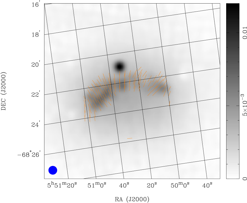
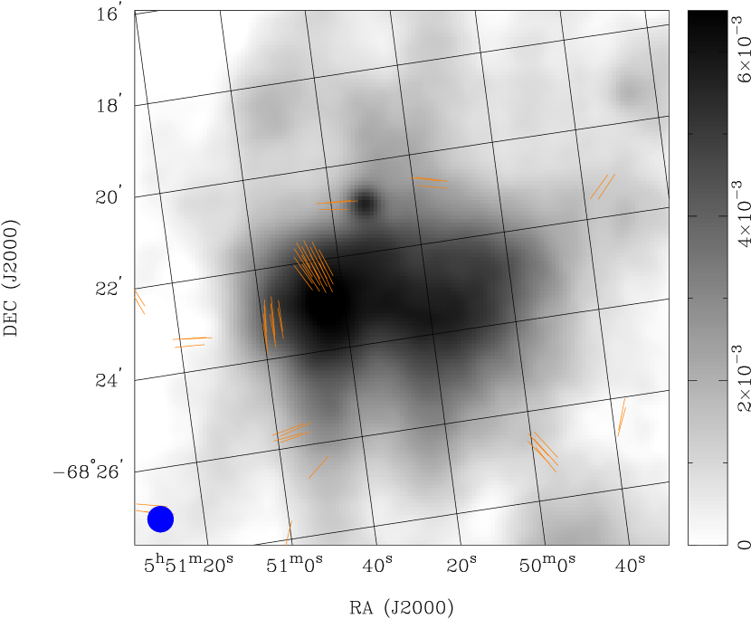
Figure 9: Images of the area around a supernova remnant and extragalactic background source in the LMC at a) 4.8 GHz and b) 8.6 GHz. The greyscales are the total intensities with the units on the wedges in Jy beam^-1. The lines represent the polarization electric vectors. The 8.6-GHz image is shown with the same resolution as the 4.8-GHz one for direct comparison. The half-power beamwidth is shown in the bottom left corners.

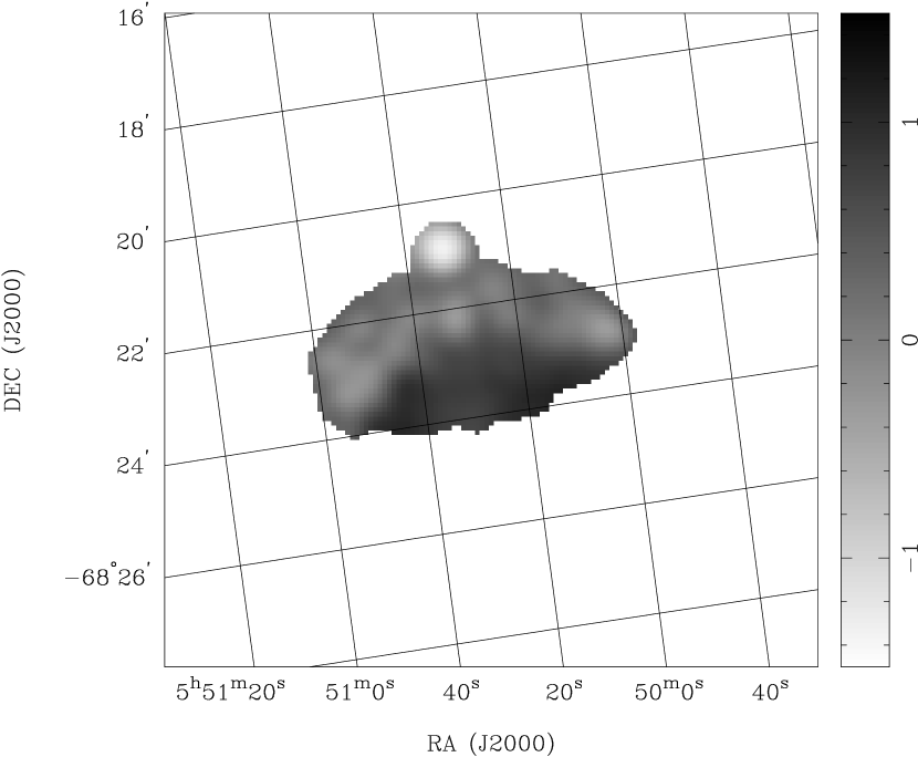
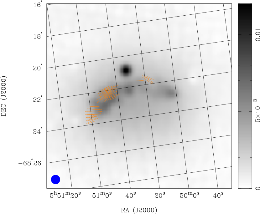
Figure 10: a) Spectral index map of a supernova remnant and background source in the LMC. The units on the wedge are the spectral index, $\alpha$, as defined in the text. b) Total intensity map at 4.8 GHz with superposed vectors representing the magnetic field directions and the polarized intensity at 4.8 GHz. The units on the wedge are Jy beam^-1.

A second interesting area is on the eastern edge of the LMC at $05^{h}50.5^{m}$ and $-68^{\circ}22^{\prime}$. In Figure 9 a,b we see a polarized curved arc which trails off to the south and a small-diameter source just to the north of the center of the arc. The north source slightly broadens the 20″ response of the beam at 8.6 GHz suggesting that it has a diameter of 10 $\pm$ 5 arcsec. Figure 10 shows the result of determining the spectral index from the match-filtered images at 4.8 and 8.6 GHz. Where the arc is bright enough to be above the noise on the southern edge, it has a spectral index, $\alpha$, of about $-$0.4 (where the flux density $S_{f}\propto f^{\alpha}$) whereas the north source has a value near $-$1.0. The former is typical of old shell supernova remnants ($http://cats.sao.ru/snr\_spectra.html$) whereas the latter is characteristic of extragalactic sources. We note that a spectral index determination between the lower-resolution MOST image at 843 MHz and a smoothed 4.8-GHz image give the same spectral index results.

Using the polarimetry to determine the Faraday rotation and intrinsic direction of the magnetic fields, we find that the mean Faraday rotation changes rather rapidly from $-$100 rad m^-2 to +150 rad m^-2 on the eastern edge of the SNR shell but then remains relatively constant at about +50 rad m^-2 across the rest of the arc. The magnetic field directions are shown in Figure 8. It appears that the magnetic field is approximately radial on the eastern edge and then tangential around the the rest of the arc.

The X-ray emission from this region observed by Chandra (Williams et al., 2004) matches the radio emission in the arc quite closely and shows a point at the position of the small-diameter north source. A long filament, DEM L238, seen faintly in H$\alpha$ extends from about 1^∘ east of this through the area between the arc and the north source and trailing off about 10 arcmin further west. Somewhat brighter H$\alpha$ and [S II] emission are seen to the south of the arc. We conclude that the north source is probably an extragalactic background source and that the arc is a supernova remnant encountering extra material on its northern side where the shock speed is slower.

4.2 Data Availability

A variety of images and the $uv$ data are available in FITS format from the Astronomical Digital Imaging Library (ADIL) at the National Center for Supercomputing Research at the University of Illinois (http://adil.ncsa.uiuc.edu/document/04.JD.01). The available data are listed in Table 2.

4.2.1 Images

For consistency, all of the images are of the full galaxy with 4624 $\times$ 4872 5″ pixels. The displayed projection will cause some blank pixels around the edges and the valid image at 8.6 GHz will be slightly smaller than that at 4.8 GHz because of the smaller primary beam at the higher frequency.

Because most users will be interested in particular areas where more detail can be seen, subimages will also be available in the near future. The user will be able to request a central position and the size of the image. They will retain the 5″ pixels but a reference position of the center of the subimage.

The images include the full resolution total intensity at both frequencies for the ATCA data alone and for the merged ATCA and Parkes data sets. We also include the match filtered total intensity image both merged and unmerged at 8.6 GHz.

For polarization, Stokes Q and U images are available at both frequencies along with polarized intensity and position angle ones. The latter have been corrected for bias but not cutoff at any level so they are appropriate for fractional polarization determinations but any individual points below 3-4 times the rms noise level cannot be trusted. Both full resolution and convolved polarimetric data are available at 8.6 GHz.

Polarization data from Parkes were available only at 4.8 GHz and merged polarimetric images were made at that frequency. In the direction of 30 Dor, the polarizarion leakage at Parkes can reach about 0.7% so the merged polarimetry cannot be used for that source but should be ok for the rest of the galaxy.

4.2.2 Visibility Data

The calibrated $uv$ data are also available from ADIL in FITS format. They will contain all polarizations and include the long-spacing data from antenna 6. The entire data set may be downloaded in a single separate FITS file for each of the two frequencies. Each file will contain thirteen 8-MHz channels centered on the nominal frequency.

5 FUTURE USES OF THE DATA

Some of the many things that can be done with these data are listed below. We and co-workers are doing some of them but readers are encouraged to obtain the images from ADIL to use them as they wish.

• Measure flux densities and spectral indices of extended sources and classify them, making use of optical, X-ray and existing radio datasets. Reliable continuum spectral indices require an extended frequency baseline with adequately matched $uv$ coverage. By comparing to the MOST data as well (45$\arcsec$ HPBW at 843 MHz) as well (Turtle et al., 1998; McIntyre & Green, 1999) we cover a decade in frequency, which should be enough to distinguish SNRs from H II regions and provide some discrimination among non-thermal spectral indices.

• Catalogs of the sources will be used to evaluate statistical luminosities, energies, birthrates, etc. of massive stars and their SNe in the LMC.

• The typical size of known SNRs in the LMC is 30″– 8′ (Williams et al., 1999). Previous radio surveys do not have adequate resolution for comparison of the X-ray and radio morphology, but the proposed observations will. The data will enable a study of the bivariate luminosity function of SNRs.

• H II regions may follow a power-law size distribution (Kennicutt & Hodge, 1986) with most smaller than 100 pc (almost 7 arcmin) in diameter. The proposed observations will enable detection of internal structures in most of these to evaluate their excitation. With the exception of 30 Doradus, all the H II regions in the catalogs of Henize (1956) and of Davies, Elliott, and Meaburn (1976) have been resolved for the first time in the radio.

• The ROSAT X-ray mosaics of the Magellanic Clouds have revealed diffuse X-ray emission in regions with scale sizes of 10 – 10³ pc (Snowden, 1999). The larger sources include superbubbles (10² pc), supergiant shells (10³ pc), and unconfined fields ($\sim$10³ pc). The proposed continuum survey will allow us to search for nonthermal radiation associated with the diffuse X-ray emission regions and study the generation of relativistic electrons by supernova remnant shocks in a variety of environments including molecular clouds and H I shells.

• The full polarimetric capability can be used to obtain valuable Faraday rotation information on the LMC and sources within it. In addition to the SNRs such as DEM L 316, DEM L 328, and N 132D, about three dozen unresolved sources have measurable polarization. No mapping of the Faraday rotation of background sources through the LMC has been previously done.

• Data from baselines including the 6 km antenna will be used to extend the catalog of unresolved objects (Marx, Dickey, and Mebold, 1997) in terms of spatial coverage, angular resolution, frequency range and sensitivity. The proposed survey will provide more accurate positions for extragalactic radio sources (e.g., AGNs and QSOs), and produce a list of UV- and optical-bright objects, which can be used as probes for interstellar absorption line observations of physical conditions and abundances of the LMC’s ISM.

The Australia Telescope Compact Array is part of the Australia Telescope funded by the Commonwealth of Australia for operation as a National Facility, managed by CSIRO. We have benefitted from help and valuable discussions with many colleagues. They include Bob Sault, Lister Staveley-Smith, John Dickey, Uli Klein, Hélène Dickel, Robin Wark, Ray Plante, You-Hua Chu, Rosa Williams, and Brian Fields. Barry Parsons, Margaret House, and Vicki Drazenovic helped to make the many visits to the Australia Telescope very enjoyable. We appreciate valuable comments by the referee, Richard Wielebinski. JRD acknowledges support from the Campus Honors Program of the UIUC and NASA Grant NAG5-11159. RAG acknowledges support from NSF Grant AST-0228953 to BIMA.

Table 1: Field Centers for Subimages

Fig.	Field	Center Location
Id	Name	$\alpha$(J2000)	$\delta$(J2000)
a	nnee	5h41m54$\fs$30	$-$66°33′58$\farcs$92
b	nne	5h27m07$\fs$59	$-$66°40′54$\farcs$08
c	nnw	5h12m16$\fs$31	$-$66°41′36$\farcs$81
d	nnww	4h57m27$\fs$90	$-$66°36′06$\farcs$67
e	nee	5h43m33$\fs$67	$-$68°09′36$\farcs$20
f	ne	5h27m45$\fs$79	$-$68°16′55$\farcs$04
g	nw	5h11m52$\fs$32	$-$68°17′40$\farcs$23
h	nww	4h56m02$\fs$36	$-$68°11′51$\farcs$21
i	see	5h45m27$\fs$77	$-$69°44′05$\farcs$30
j	se	5h28m29$\fs$72	$-$69°51′51$\farcs$87
k	sw	5h11m24$\fs$72	$-$69°52′39$\farcs$93
l	sww	4h54m24$\fs$09	$-$69°46′28$\farcs$79
m	ssee	5h47m39$\fs$98	$-$71°17′26$\farcs$51
n	sse	5h29m20$\fs$71	$-$71°25′45$\farcs$76
o	ssw	5h10m52$\fs$68	$-$71°26′37$\farcs$22
p	ssww	4h52m30$\fs$16	$-$71°20′00$\farcs$00

Table 2: FITS Data Available

Name	Freq. (MHz)	Type	Other Attributes
Images
LMC4.8-i.a	4.8	total intensity	only ATCA
LMC4.8-i.m	4.8	total intensity	merged ATCA + Parkes
LMC4.8-i.f	4.8	total intensity	match filtered, only ATCA
LMC4.8-q.a	4.8	Stokes Q	only ATCA
LMC4.8-q.m	4.8	Stokes Q	merged ATCA + Parkes
LMC4.8-u.a	4.8	Stokes U	only ATCA
LMC4.8-u.m	4.8	Stokes U	merged ATCA + Parkes
LMC4.8-p.a	4.8	polarized intensity	only ATCA
LMC4.8-p.m	4.8	polarized intensity	merged ATCA + Parkes
LMC4.8-pa.a	4.8	e-vector position angle	only ATCA
LMC4.8-pa.m	4.8	e-vector postion angle	merged ATCA + Parkes
LMC8.6-i.a	8.6	total intensity	only ATCA
LMC8.6-i.m	8.6	total intensity	merged ATCA + Parkes
LMC8.6-i.f	8.6	total intensity	match filtered, only ATCA
LMC8.6-i.f.m	8.6	total intensity	match filtered, merged
LMC8.6-q.a	8.6	Stokes Q	only ATCA
LMC8.6-q.c	8.6	Stokes Q	convolved
LMC8.6-u.a	8.6	Stokes U	only ATCA
LMC8.6-u.c	8.6	Stokes U	convolved
LMC8.6-p.a	8.6	polarized intensity	only ATCA
LMC8.6-p.c	8.6	polarized intensity	convolved
LMC8.6-pa.a	8.6	e-vector position angle	only ATCA
LMC8.6-pa.c	8.6	e-vector position angle	convolved
UV data
LMC4.8-uv	4.8	full Stokes	calibrated, all 6 antennas
LMC8.6-uv	8.6	full Stokes	calibrated, all 6 antennas

Figure 1: Sample observing patterns for the lower right field within one tile and parts of the adjoining fields. The circles and boxes represent the 6-row patterns and the Xs and crosses represent the 5-row patterns within the field. The separations between points are shown.

Figure 6: A detailed figure showing the 8640 MHz emission from the region around 30 Doradus. The units on the wedge are Jy beam^-1. The field of view is 1/16 of the total LMC mosaic. Figures 6a-p show detailed subregions across the entire LMC but are presented in the electronic edition only. Central coordinates for each subregion are given in Table 1.

References

- Australia Telescope (1992) Australia Telescope 1992, J. Electrical Electronics Engineering, Australia, 12, No 2
- Bode (1801) Bode, J. 1801, Allgemeine Beschreibung und Nachweisung der Gestirne, (Berlin: private publisher)
- Briggs (1995) Briggs, D. S. 1995, BAAS, 27, 1444
- Davies et al. (1976) Davies, R., Elliott, K., & Meaburn, J. 1976, MemRAS, 81, 89
- Dickel and Milne (1995) Dickel, J. & Milne, D. 1995, AJ, 109, 200
- Dickel and Milne (1998) Dickel, J. & Milne, D. 1998, AJ, 115, 105
- Filipovic et al. (1995) Filipovic, M., Haynes, R., White, G., Jones, P., Klein, U., & Wielebinski, R. 1995, A&AS, 111 311
- Haynes et al. (1991) Haynes, R., Klein, U.,Wayte, S., Wielebinski, R., Murray, J., Bajaja, E., Meinert, D., Buczilowski, U., Harnett, J., Hunt, A., Wark, R., & Sciacca, L. 1991, A&A, 252, 475
- Henize (1956) Henize, K. 1956, ApJS, 2, 315
- Kennicutt & Hodge (1986) Kennicutt, R. and Hodge, P. 1986, ApJ, 306, 130
- Killeen et al. (1986) Killeen, N. E. B., Bicknell, G., & Ekers, R. D. 1986, ApJ, 302, 306
- Klein et al. (1993) Klein, U., Haynes, R., Wielebinski, R., & Meinert, D. 1993, A&A, 271, 402
- Klinger et al. (2002) Klinger, R., Dickel, J., Fields, B., & Milne, D. 2002, AJ, 124, 2135
- Kothes et al. (1998) Kothes, R., Reich, W., & Fuerst, E. 1998, A&A, 331, 661
- Lazendic et al. (2000) Lazendic, J. S., Dickel, J. R., Haynes, R. F., Jones, P. A., & White, G. L. 2000, ApJ, 540, 808
- Lazendic et al. (2003) Lazendic, J. S., Dickel, J. R., & Jones. P. A. 2003, ApJ, 596, 287
- Marx et al. (1997) Marx, M., Dickey, J. and Mebold, U. 1997, A&AS, 126, 325
- McIntyre & Green (1999) McIntyre, V. & Green, A. 1999, private communication
- Sault et al. (1995) Sault, R. J., Teuben, P. J., & Wright, M. C. H. 1995, in R.A. Shaw, H.E. Payne, and J.J.E. Hayes, eds., Astronomical Data Analysis Software and Systems IV, ASP Conference Series 77, 433
- Smith (1999) Smith, R. C. 1999, in Chu et al. eds., New Views of the Magellanic Clouds, IAU Symposium 190, 28
- Snowden (1999) Snowden, S. 1999, in Chu et al. eds., New Views of the Magellanic Clouds, IAU Symposium 190, 32
- Turtle et al. (1998) Turtle, A., Ye, T., Amy, S., & Nichols, J. 1998, PASA, 15, 280
- Vinokur (1965) Vinokur, M. 1965, AnAp, 28, 412
- Williams et al. (1999) Williams, R., Chu, Y.-H., Dickel, J., Petre, R., Smith, R., & Tavarez, M. 1999, ApJS, 123, 467
- Williams et al. (2004) Williams, R., Chu, Y.-H., Dickel, J., Gruendl, R., Guerrero, M., Seward, F., & Hobbs, G. 2004, “Supernova Remnants in the Magellanic Clouds. V. The Complex Interior Structure of the N206 SNR,” ApJ, submitted