Line formation in solar granulation

The solar photospheric carbon abundance has been determined from [C i], C i, CH vibration-rotation, CH A-X electronic and C₂ Swan electronic lines by means of a time-dependent, 3D, hydrodynamical model of the solar atmosphere. Departures from LTE have been considered for the C i lines. These turned out to be of increasing importance for stronger lines and are crucial to remove a trend in LTE abundances with the strengths of the lines. Very gratifying agreement is found among all the atomic and molecular abundance diagnostics in spite of their widely different line formation sensitivities. The mean of the solar carbon abundance based on the four primary abundance indicators ([C i], C i, CH vibration-rotation, C₂ Swan) is ${\rm log}\,\epsilon_{\rm C}=8.39\pm 0.05$, including our best estimate of possible systematic errors. Consistent results also come from the CH electronic lines, which we have relegated to a supporting role due to their sensitivity to the line broadening. The new 3D based solar C abundance is significantly lower than previously estimated in studies using 1D model atmospheres.

1 Introduction

Carbon is a crucial element for the emergence of life in the Universe as we know it. Furthermore, it is one of the most abundant elements in the cosmos behind only hydrogen, helium and oxygen in this respect. While it is clear that carbon is produced through the $3\alpha$-reaction (Burbidge et al. 1957) in stellar interiors, a debate regarding the exact site of its production is still ongoing. Recently both low- and intermediate mass stars as well as massive stars have been advocated to be the primary sources of the element (e.g. Chiappini et al. 2003; Akerman et al. 2004). Carbon also plays a key role in the physics of the interstellar medium for example through its propensity to form dust (e.g. Dopita & Sutherland 2002; Lodders 2003).

In view of its rather special status in astrophysics, it is clearly of particular importance to ascertain the traditional abundance anchorage point, namely the solar carbon abundance. In the standard reference of Anders & Grevesse (1989) the solar carbon abundance is quoted as ${\rm log}\,\epsilon_{\rm C}=8.56\pm 0.04$, which was subsequently revised to ${\rm log}\,\epsilon_{\rm C}=8.52\pm 0.06$ by Grevesse & Sauval (1998) based on a re-analysis of various atomic and molecular lines using a temperature-modified Holweger-Müller (1974) 1D semi-empirical model atmosphere. Holweger (2001) preferred the slightly higher value of ${\rm log}\,\epsilon_{\rm C}=8.59\pm 0.11$ based only on permitted C i lines in the optical and infrared (IR). In sharp contrast to these results, Allende Prieto et al. (2002) found the much lower value ${\rm log}\,\epsilon_{\rm C}=8.39\pm 0.04$ through a detailed study of the forbidden [C i] line at 872.7 nm employing a state-of-the-art 3D time-dependent hydrodynamical model of the solar photosphere (Asplund et al. 2000b). This latter value is in good agreement with the evidence from nearby B stars (Sofia & Meyer 2001), local interstellar medium (Meyer et al. 1998; André et al. 2003), the solar corona and the solar wind (Murphy et al. 1997; Reames 1999), in particular in view of the recent downward revision of the solar oxygen abundance (Allende Prieto et al. 2001; Asplund et al. 2004, hereafter Paper IV).

While the [C i] 872.7 nm line has a well-determined transition probability and should be robust against departures from LTE, its relative weakness and the possible presence of weak blends may cast some doubt on the reliability of the low carbon abundance derived by Allende Prieto et al. (2002). We here present a comprehensive study of other available carbon diagnostics, including permitted atomic and various molecular lines using the same 3D hydrodynamical solar model atmosphere. Our results corroborate the findings of Allende Prieto et al. and unambiguously point to a significant revision by $-0.17$ dex of the solar carbon abundance compared with the often-adopted value given in Anders & Grevesse (1989). It is noteworthy that only with a 3D analysis are the primary atomic and molecular abundance criteria in excellent agreement, which further strengthens our conclusions.

2 Analysis

2.1 Atomic and molecular data

[C i] line: Recent calculations of the transition probability of the [C i] 872.7 nm line have apparently converged to $A=0.640$ s^-1 or log $gf=-8.136$ (Hibbert et al. 1993; Galavis et al. 1997). The central wavelength of the line is used as a free parameter in the $\chi^{2}$ analysis of the profile fitting described below, which results in a rest wavelength of $872.7139\pm 0.0004$ nm when taking into account the predicted convective blue-shift of the line. The lower level excitation potential of the line is $1.264$ eV (Bashkin & Stoner 1975).

C i lines: The transition probabilities for the selected 16 permitted C i lines which represent our primary line list were taken from Hibbert et al. (1993). The VALD (Piskunov et al. 1995; Kupka et al. 1999) and NIST (Wiese et al. 1996) databases provided the necessary data for excitation potential, radiative broadening and central wavelengths. Collisional broadening by H was computed according to the tabulations in Anstee & O’Mara (1995), Barklem & O’Mara (1997) and Barklem et al. (1998), except for C i 505.2, 538.0, 658.7, 3085.4 and 3406.5 nm which fall outside the table boundaries. For those lines the classical Unsöld (1955) recipe with an enhancement factor $E=2.0$ was used. The corresponding uncertainty is however minor: with $E=1.0$ the derived abundances for the three optical lines would be about 0.01 dex higher while for the two IR lines the corresponding error is about 0.03 dex.

We initially considered additional C i lines, which however were all rejected in the final analysis for various reasons, such as suffering from blends (e.g. 477.5, 1186.3 nm), too large sensitivity to velocity and/or pressure broadening (e.g. 965.8, 1068.5, 1070.7, 1189.5, 1744.8, 3372.8 nm) or uncertain continuum placement (e.g. 1184.8 nm). We stress that it is better to retain only the best quality abundance indicators than using a larger sample of less reliable lines. Nevertheless, our line list is sufficiently large to secure a final mean abundance that is insensitive to possible problems with a few individual lines.

CH vibration-rotation and electronic lines: The analysis is based on the best 102 vibration-rotation lines of the (1,0), (2,1) and (3,2) bands in the infrared ($3.3-3.8\,\mu$m). We also include, with a lower weight, nine apparently clean weak lines from the (0,0) and (1,1) bands of CH A-X around 430 nm (6 and 3 lines, respectively). The dissociation energy of CH is well-known: $D_{0}{\rm(CH)}=3.465$ eV (Huber & Herzberg 1979). The partition functions and statistical weights for CH are taken from Sauval & Tatum (1984) for consistency with the adopted dissociation energy and equilibrium constants. The lower level excitation potentials for the CH lines were adopted from Mélen et al. (1989) and the transition probabilities from Follmeg et al. (1987). The latter are the same as used by Grevesse et al. (1991). The band oscillator strengths for the CH A-X lines are $f_{00}=(5.16\pm 0.11)\cdot 10^{-3}$ and $f_{11}=(4.46\pm 0.15)\cdot 10^{-3}$ (Larsson & Siegbahn 1986). As the quantum mechanical approach for pressure broadening outlined by O’Mara and collaborators (e.g. Anstee & O’Mara 1995) is not applicable to molecular transitions, we have resorted to the classical Unsöld (1955) recipe with an enhancement factor of 2 for all molecular lines. The particular choice of enhancement factor has no impact on the derived abundances however for these lines.

C₂ electronic lines: We selected the 17 least blended weak C₂ lines from the (0,0) $d^{3}\Pi_{g}-a^{3}\Pi_{u}$ Swan band. Our adopted dissociation energy of C₂ comes from the accurate experimental measurement by Urdahl et al. (1991): $D_{0}{\rm(C_{2})}=6.297$ eV. This laboratory determination is in very good agreement with the theoretical calculations of Pradham et al. (1994) which suggests $D_{0}{\rm(C_{2})}=6.27$ eV. Our value is 0.09 eV higher than that recommended by Huber & Herzberg (1979) and 0.19 eV higher than the value employed by Lambert (1978) in his classical solar abundance analysis of CNO. We remind the reader that the derived carbon abundance from C₂ lines depends on the dissociation energy as $\Delta{\rm log}\epsilon_{\rm C}\approx-\Delta D_{0}/2$. The C₂ partition functions and equilibrium constants have been adopted from Sauval & Tatum (1984). The C₂ Swan band oscillator strengths are well-determined from measurements of the radiative lifetime of the $d^{3}\Pi_{g}$ state (see Grevesse et al. 1991). As for the CH lines, we use an enhancement factor of 2 to the Unsöld recipe for pressure broadening, which however has no influence on the final results. We do not consider the lines of the C₂ Phillips system to be sufficiently reliable for our purposes and hence do not include any such lines in the analysis.

CO vibration-rotation lines: In principle, CO lines can be utilised to derive the carbon abundance whenever the oxygen abundance has first been determined accurately from alternative diagnostics. We will not consider CO in this analysis, however, due to their large model atmosphere sensitivity through the high dissociation energy which makes them less reliable than other diagnostics. Indeed, no available 1D hydrostatic model atmosphere, be it semi-empirical like the Holweger-Müller (1974) or VAL-3C (Vernazza et al. 1976) models or theoretical like the marcs (Gustafsson et al. 1975 and subsequent updates) or Kurucz (1993) models, have been able to explain the strong CO lines observed in the Sun (not counting of course semi-empirical models specifically constructed to reproduce the CO lines, such as the models described by Grevesse & Sauval 1991, 1994, Grevesse et al. 1995 and Avrett 1995). This has been taken as evidence for a very cool temperature structure or evidence for a temperature bifurcation of the gas in the upper photosphere/lower chromosphere (e.g. Ayres 2002 and references therein). Uitenbroek (2000a,b) has shown that the situation has improved with the advent of 1D time-dependent hydrodynamical atmosphere models which account for important non-LTE effects (Carlsson & Stein 1992, 1995, 1997) and 3D hydrodynamical models like those described herein. Indeed, with the same 3D model as used here the long-standing COnundrum may finally be about to be resolved (Asensio Ramos et al. 2003). We intend to return to the CO lines in a future investigation in this series.

2.2 Observational data

Throughout we use disk-center ($\mu=1.0$ for the optical lines and $\mu=0.935$ for molecular lines in the IR) intensity observations. In the optical wavelength region the Brault & Neckel (1987, see also Neckel 1999) solar atlas has been employed. This high-quality atlas was recorded with the Fourier Transform Spectrograph at Kitt Peak Observatory at a resolving power of about 500,000 and a signal-to-noise exceeding 1000 at all wavelength regions of interest here. Minor adjustments to the tabulated continuum level immediately surrounding the relevant spectral lines were made. In some cases the Kitt Peak FTS atlas was supplemented with the Jungfraujoch disk-center solar atlas (Delbouille et al. 1973) when lines were affected by telluric lines (e.g. C i 711.1 and 960.3 nm). For the four lines between 1254 and 1259 nm we used the infrared solar atlas of Delbouille et al. (1981) also recorded at Kitt Peak. For the analysis of the last four C i lines in Table 1 and the CH vibration-rotation lines the Spacelab-3 atmos solar disk-center intensity IR observations has been used (Farmer & Norton 1989, see also Farmer 1994). The resolving power of the atmos atlas is about 200,000. The $S/N$ varies with wavelength but is typically at least 400 in the regions of interest here.

A major advantage with the new generation of 3D hydrodynamical model atmospheres employed here is the in general excellent agreement between predicted and observed line profiles without resorting to the usual micro- and macroturbulence necessary in 1D spectrum synthesis (e.g. Asplund et al. 2000a,b,c). This facilitates the use of line profile fitting for individual lines for the carbon abundance determination, a method that we apply here to the analysis of the atomic lines. Since the line profile fitting procedure is more ambiguous in the 1D case due to the poorer agreement between predicted and observed profiles, we here adopt the theoretical line intensities from the 3D profile fitting as “observed” equivalent widths for the 1D spectrum synthesis (we note that these values are in excellent agreement with those directly measured on the observed spectra). This enables a direct comparison of the effects stemming from the choice of 1D or 3D model atmospheres. Due to the sheer number of molecular lines employed in the present study, we rely for practical reasons on the measured equivalent widths for both the 1D and 3D abundance analyses of the molecular transitions. The equivalent widths of the molecular lines have been obtained by fitting Gaussians to the observed profiles. Various tests have ensured that no significant error has been introduced by the use of fitting Gaussians rather than for example a Lorentz profile for these particular lines.

2.3 LTE spectral line formation

We follow the same procedure as in previous articles in the present series (Asplund et al. 2000b,c; Asplund 2000; Asplund et al. 2004; Asplund 2004; hereafter Papers I, II, III, IV, V) of studies of spectral line formation in the solar granulation. We employ a 3D, time-dependent, hydrodynamical simulation of the solar surface convection as a realistic model of the solar atmosphere. The reader is referred to Stein & Nordlund (1998) and Paper I for further details of the construction of the 3D solar model atmosphere. For comparison purposes, we have also performed identical calculations employing two widely-used 1D hydrostatic models of the solar atmosphere: the semi-empirical Holweger-Müller (1974) model and a theoretical, LTE, line-blanketed marcs model (Asplund et al. 1997).

Equipped with the 3D hydrodynamical solar atmosphere, 3D spectral line formation calculations have been performed for [C i], C i, CH, and C₂ lines under the simplifying assumptions of LTE. In addition, instantaneous chemical equilibrium (ICE) has been assumed valid for the molecule formation. This is a potentially serious issue since in a stellar atmosphere the time-scale for molecule formation could be longer than the corresponding dynamical time-scale and hence the actual molecular number densities may be out of equilibrium (e.g. Uitenbroek 2000a,b). To our knowledge, the only published study devoted to follow the time-dependent chemical evolution using a reaction network is that of Asensio Ramos et al. (2003) who investigated CO in the Sun. They concluded that ICE is an acceptable approximation below heights of about 700 km. Since our CH and C₂ lines are formed in much deeper layers, this assumption is unlikely to significantly affect our derived C abundances (see also Asensio Ramos & Trujillo Bueno 2003). However, we stress that only detailed chemical evolution calculations can confirm whether this conclusion is correct. While such computations are beyond the scope of the present study, we intend to investigate this in a forthcoming publication. Finally we note for completeness that in principle it is necessary to use the non-LTE populations of H and C when estimating the number densities of CH and C₂ even under the assumption of ICE. Fortunately, both elements are predominantly populated by their ground states for which LTE is an excellent assumption in the relevant parts of the solar atmosphere. Therefore the use of the Saha distribution when computing the atomic partial pressures needed for estimating the molecular densities is fully justified.

The spectrum synthesis employs realistic equation-of-state and continuous opacities (Gustafsson et al. 1975 and subsequent updates; Mihalas et al. 1988). The temporal coverage of the part of the solar simulation which forms the basis of the line formation computations is 50 min of solar-time with snapshots every 30 s. The comparison with observations relates to disk-center intensity profiles ($\mu=1.0$ and $\mu=0.935$ depending on the line). As the calculations self-consistently account for the Doppler shifts arising from the convective motions, no micro- or macroturbulence enter the 3D spectral synthesis. In the absence of such convective line broadening, all 1D calculations have been performed adopting a microturbulence $\xi_{\rm turb}=1.0$ km s^-1 unless noted otherwise (e.g. Holweger & Müller 1974: Blackwell et al. 1995).

2.4 Non-LTE spectral line formation

While non-LTE effects are expected to be modest for the other carbon abundance diagnostics, the same can not be assumed for the high-excitation permitted C i lines employed here. In order to investigate this further we have performed detailed non-LTE calculations based on the Holweger-Müller and marcs 1D model atmospheres. Full 3D non-LTE line formation computations have recently been carried out for Li (Asplund et al. 2003) and O (Paper IV) for a couple of snapshots from the same solar simulation as employed here. As described below, the requirement for a very extensive carbon model atom to obtain realistic results currently prevents similar calculations for this element. Until such a 3D non-LTE study is performed we will have to rely on the results from the corresponding 1D case, which, however, is expected to yield sufficiently accurate results for these high-excitation lines formed in deep atmospheric layers. In this connection, we note the very similar non-LTE abundance corrections obtained in 3D and 1D for O i lines of similar character as the C i lines (Paper IV; Allende Prieto et al. 2004). We intend to return to the issue of 3D non-LTE line formation for C i lines in a later study.

Our carbon model atom consists of 217 levels in total, of which 207 belong to C i, nine to C ii and one represents C iii. The atom is complete up to principal quantum number $n=9$ for the singlet and triplet systems with no fine structure of the terms accounted for. The highest C i level corresponds to an excitation potential $\chi_{\rm exc}=11.13$ eV, which is only 0.13 eV below the ionization limit. The energy levels are taken from the experimental data of Bashkin & Stoner (1975). The levels are coupled radiatively through 458 bound-bound and 216 photo-ionization transitions with the data coming from the Opacity Project database TOPbase (Cunto et al. 1993). Excitation and ionization due to collisions with electrons are accounted for through the impact approximation for radiatively allowed transitions and the van Regemorter (1962) formalism for forbidden lines adopting an oscillator strength $f=0.01$. No inelastic hydrogen collisions are included as the available laboratory measurements and quantum mechanical calculations suggest that the normally employed recipe (Drawin 1968, see also Steenbock & Holweger 1984) over-estimates the collisional cross-sections by about three orders of magnitude (Fleck et al. 1991; Belyaev et al. 1999; Barklem et al. 2003). We do note, however, that there is some astrophysical evidence that this is not the case for O (e.g. Allende Prieto et al. 2004). In the absence of suggestions to the contrary for C, we prefer not to employ the Drawin formula given the uncertainties involved. The 1D non-LTE calculations have been performed using the statistical equilibrium code multi (Carlsson 1986), version 2.2. The non-LTE abundance corrections have been interpolated from the non-LTE and LTE equivalent widths for four different abundances (log $\epsilon_{\rm C}=8.30,8.40,8.50,8.60$). The corresponding LTE results necessary for estimating the non-LTE abundance corrections were also obtained with multi using a model atom with all collisional cross-sections artificially set to extremely large values to ensure full thermalization of all levels and transitions.

Table 1 lists the resulting non-LTE abundance corrections for the Holweger-Müller and marcs 1D model atmospheres. Clearly, the non-LTE effects are not particularly dependent on the employed model atmosphere, at least not within the framework of 1D models. While the four lowest C i levels (2p^{2 3}P, 2p^{2 1}D, 2p^{2 1}S, 2p^{3 5}S^o) are all perfectly described by the Boltzmann distribution due to close collisional coupling, the next two levels (3s ³P^o, 3s ¹P^o) are slightly over-populated relative to the LTE expectation, as seen in Fig. 1. The vast majority of levels, however, show a very similar behaviour with small but significant underpopulations in the typical line-forming regions ($-1\la\log\tau_{500}\la 0$ according to the line depression contribution functions introduced by Magain 1986): $\beta_{\rm i}\equiv n_{\rm i}/n_{\rm i}^{\rm LTE}<1$. The similarity of the levels with $\chi_{\rm exc}>8.5$ eV is mainly due to efficient collisional interlocking. In all cases, the non-LTE abundance corrections for the here employed C i lines are negative (i.e. the lines become stronger in non-LTE than in LTE), since the line source function exceeds the Planck function $S_{\rm l}/B_{\nu}\approx\beta_{\rm up}/\beta_{\rm low}<1$ in the line-forming regions. In addition, many of the C i lines originate from the 3s ³P^o or 3s ¹P^o levels which are slightly over-populated ($\beta_{\rm low}>1$) which increases the line opacity and hence strengthens the lines further. The abundance corrections show a clear dependence on equivalent width with the largest corrections obtained for the strongest lines. Our non-LTE abundance corrections would have been significantly smaller ($<0.05$ dex) had we included H collisions through the classical Drawin (1968) formula. Our non-LTE results are qualitatively the same as those obtained by Stürenbock & Holweger (1990) but show in general slightly larger non-LTE effects, mainly due to our larger atom, more realistic photo-ionization cross-sections and no inclusion of efficient H collisions.

Figure 1: The departure coefficients $\beta_{\rm i}=n_{\rm i}/n_{\rm i}^{\rm LTE}$ for the C i levels as a function of continuum optical depth in the marcs model atmosphere; the corresponding case for the Holweger-Müller model is almost identical. The four lowest levels (dotted lines) show no departures from LTE, while the following two levels (dashed lines) experience a slight over-population in the line-forming region. The majority of levels, however, have a small under-population (solid lines), as does the ground state of C ii (solid line connected with stars).

Table 1: The computed non-LTE abundance corrections of C i lines for the Holweger-Müller (1974) model and marcs (Asplund et al. 1997) 1D model atmospheres. The departures from LTE have been estimated using multi (Carlsson 1986) and a 217-level model atom.

line		$\chi_{\rm exc}$	log $gf$	$\Delta({\rm log}\epsilon_{\rm C})$
[nm]		[eV]		HM	marcs
505.2167	3s1P${}^{\rm o}_{1}$ – 4p1D2	7.685	-1.304	-0.05	-0.04
538.0337	3s1P${}^{\rm o}_{1}$ – 4p1P1	7.685	-1.615	-0.04	-0.03
658.7610	3p1P1 – 4d1P${}^{\rm o}_{1}$	8.537	-1.021	-0.03	-0.03
711.1469	3p3D1 – 4d3F${}^{\rm o}_{2}$	8.640	-1.074	-0.04	-0.04
711.3179	3p3D3 – 4d3F${}^{\rm o}_{4}$	8.647	-0.762	-0.05	-0.05
960.3036	3s3P${}^{\rm o}_{0}$ – 3p3S1	7.480	-0.895	-0.15	-0.15
1075.3976	3s3P${}^{\rm o}_{2}$ – 3p3D1	7.488	-1.598	-0.11	-0.10
1177.7546	3p3D2 – 3d3F${}^{\rm o}_{2}$	8.643	-0.490	-0.11	-0.09
1254.9493	3p3P0 – 3d3P${}^{\rm o}_{1}$	8.847	-0.545	-0.09	-0.08
1256.2124	3p3P1 – 3d3P${}^{\rm o}_{0}$	8.848	-0.504	-0.09	-0.08
1256.9042	3p3P1 – 3d3P${}^{\rm o}_{1}$	8.848	-0.586	-0.09	-0.08
1258.1585	3p3P1 – 3d3P${}^{\rm o}_{2}$	8.848	-0.509	-0.09	-0.08
2102.3151	3p1S0 – 3d1P${}^{\rm o}_{1}$	9.172	-0.437	-0.08	-0.06
2290.6565	3p1S0 – 4s1P${}^{\rm o}_{1}$	9.172	-0.182	-0.10	-0.08
3085.4621	3d1F${}^{\rm o}_{3}$ – 4p1D2	9.736	0.086	-0.05	-0.05
3406.5790	4p1P1 – 4d1D${}^{\rm o}_{2}$	9.989	0.454	-0.11	-0.10

3 The solar photospheric C abundance

3.1 The forbidden [C i] 872.7 nm line

The forbidden [C i] 872.7 nm line has been studied in detail by Allende Prieto et al. (2002) using the same 3D hydrodynamical solar model atmosphere as employed here. They determined the carbon abundance from a $\chi^{2}$-analysis of the solar flux atlas of Kurucz et al. (1984) with three free parameters besides the carbon abundance: the wavelength of the [C i] line (see discussion in Sect. 2.1), continuum placement and log $gf\cdot\epsilon_{\rm Si}$ for the Si i 872.80 nm line of which the [C i] line is located in its blue wing. Including fitting errors and estimates of possible systematic errors, they arrived at ${\rm log}\,\epsilon_{\rm C}=8.39\pm 0.04$.

For consistency with the analysis of the permitted lines, we have re-analysed the forbidden line using the disk-center intensity profile instead of the flux profile. The derived carbon abundance, however, is not affected by this choice: ${\rm log}\,\epsilon_{\rm C}=8.39\pm 0.04$. We note that Lambert & Swings (1967) flagged a potential blending Fe i line, which, if contributing to the feature, would imply a downward revision of our derived carbon abundances. Using other Fe i lines belonging to the same multiplet, Allende Prieto et al. (2002) estimated the equivalent width of the line to be $<0.03$ pm (1 pm $\equiv$ 10 mÅ), which corresponds to a downward change of $<0.02$ dex for the derived carbon abundance.

The best fit carbon abundance results in a theoretical disk-center intensity equivalent width of 0.53 pm. Employing this value, the 1D Holweger-Müller model atmosphere implies a carbon abundance of ${\rm log}\,\epsilon_{\rm C}=8.45\pm 0.04$ (adopting the same error estimate as for the 3D analysis), while the marcs model suggests ${\rm log}\,\epsilon_{\rm C}=8.40\pm 0.04$. Clearly, this particular transition is relatively insensitive to the choice of model atmosphere.

3.2 Permitted C i lines

Table 2: The derived solar carbon abundance as indicated by the forbidden [C i] 872.7 nm transition and permitted C i lines. The results include the non-LTE abundance corrections presented in Table 1. In the absence of detailed 3D non-LTE calculations for C i, the 1D non-LTE corrections for the marcs model atmosphere has here been used also for the 3D case.

line	$\chi_{\rm exc}$	log $gf$	3Da	$W_{\lambda}^{\rm b}$	HMc	marcsc
[nm]	[eV]			[pm]
[C i]:
872.71	1.264	-8.136	8.39	0.53	8.45	8.40
C i:
505.2167	7.685	-1.304	8.34	4.07	8.40	8.34
538.0337	7.685	-1.615	8.36	2.52	8.42	8.38
658.7610	8.537	-1.021	8.31	1.79	8.37	8.33
711.1469	8.640	-1.074	8.30	1.37	8.35	8.32
711.3179	8.647	-0.762	8.40	2.85	8.45	8.41
960.3036	7.480	-0.895	8.35	9.60	8.34	8.32
1075.3976	7.488	-1.598	8.37	4.69	8.38	8.36
1177.7546	8.643	-0.490	8.38	6.69	8.38	8.36
1254.9493	8.847	-0.545	8.39	5.90	8.41	8.37
1256.2124	8.848	-0.504	8.39	6.24	8.41	8.37
1256.9042	8.848	-0.586	8.39	5.59	8.41	8.37
1258.1585	8.848	-0.509	8.37	6.13	8.40	8.36
2102.3151	9.172	-0.437	8.42	8.76	8.44	8.39
2290.6565	9.172	-0.182	8.33	11.88	8.34	8.30
3085.4621	9.736	0.086	8.35	5.53	8.36	8.34
3406.5790	9.989	0.454	8.34	7.09	8.34	8.34

• The abundances derived using the 3D model atmosphere have been obtained from profile fitting of the observed lines.

• The predicted disk-center intensity equivalent widths with the 3D model atmosphere using the best fit abundances shown in the fourth column.

• The derived abundances with the Holweger-Müller (1974) and the marcs (Asplund et al. 1997) 1D hydrostatic model atmospheres in order to reproduce the equivalent widths presented in the fifth column.

The carbon abundance determination using permitted atomic lines is based on the 16 C i lines listed in Table 2. The individual abundances have been estimated using profile fitting for disk-center intensity; we note for completeness that very similar abundances would have been derived had flux profiles been used instead. The profile fitting has been performed for the spatially and temporally averaged 3D LTE line calculations from the 100 snapshots used. As clear from Fig. 2 the agreement between predicted and observed profiles is very satisfactory. In contrast, the theoretical line profiles in 1D require additional broadening from macroturbulence to get the correct line widths but of course the observed line shifts and asymmetries can not be accounted for.

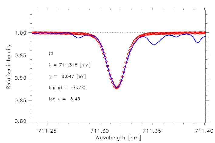
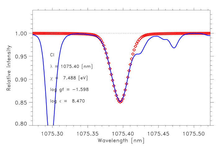
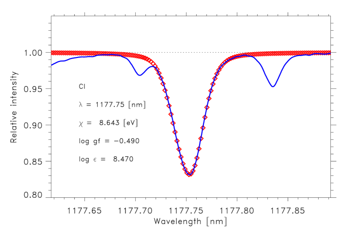
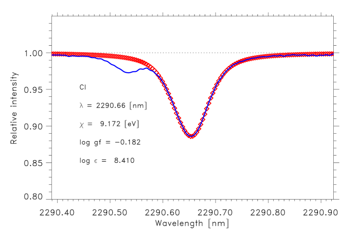
Figure 2: The predicted 3D LTE profiles of the C i 711.3, 1075.4, 1177.7 and 2290.6 nm lines (diamonds) compared with the solar intensity atlas (solid lines, Brault & Neckel 1987 for the first three lines and Farmer & Norton 1989 for the last line). The excellent agreement is achieved without any micro- or macroturbulence due to the Doppler shifts arising from the convective motions.

Due to the large carbon model atom required to capture the essence of the non-LTE effects, 3D non-LTE line formation computations for the C i lines have not been possible. As a substitute, we apply the 1D non-LTE abundance corrections estimated with the marcs model atmosphere given in Table 1 to the 3D LTE abundance estimates to arrive at our final results presented in Table 2. It is worthwhile pointing out that the similarities between the 1D non-LTE results for the marcs and Holweger-Müller model atmospheres, in spite of their quite different temperature structures (see Fig. 2 in Paper IV), give reasons to believe that the 3D non-LTE case would indeed be similar as well had it been available.

Figure 3: The derived solar carbon abundance from permitted C i lines using the 3D hydrodynamical model atmosphere as a function of equivalent width (Upper panel). The filled circles denote the case when the 1D marcs-based non-LTE abundance corrections in Table 1 have been applied, while the open circles correspond to the LTE results. Also shown are the corresponding cases with the Holweger-Müller (Middle panel) and the marcs (Lower panel) 1D model atmospheres, which display similar trends with equivalent widths. As explained in the text, this may signal underestimated non-LTE effects.

The mean C i-based solar carbon non-LTE abundance is ${\rm log}\,\epsilon_{\rm C}=8.36\pm 0.03$ (standard deviation). The scatter is encouragingly small. There is no trend in the derived abundances with either wavelength or excitation potential although as seen in Fig. 3 there is a small correlation with the strengths of the lines (about 0.04 dex from the weakest to the strongest lines, i.e. $W_{\lambda}=1-12$ pm). One possibility is that the line broadening arising from the Doppler shifts due to the convective motions are underestimated, akin to using too small a microturbulence in 1D. Our previous 3D LTE analysis of Fe i lines have revealed a similar trend (Asplund et al. 2000c). However it should be pointed out that that correlation could also be the result of neglecting departures from LTE (Shchukina & Trujillo Bueno 2001), and there is no corresponding trend for Fe ii or Si i lines (Asplund 2000), which would be expected if the convective line broadening is underestimated. From Fig. 3 it is clear that the trend with equivalent width is largely driven by the two weakest lines, 658.7 and 711.1 nm. Although the former line is located in the far wing of the H$\alpha$ line and there are some telluric H₂O lines around the latter, we have not been able to identify any obvious explanation for these two abundances being underestimated.

In our opinion, the most likely explanation for this slight correlation is underestimated non-LTE corrections in the 3D case. We note that we have here adopted the non-LTE calculations from the 1D marcs model in the lack of suitable full 3D non-LTE calculations. It is quite conceivable that the presence of temperature inhomogeneities could produce slightly more pronounced non-LTE effects, in particular for the stronger lines. Fortunately, this residual trend is very small and will not affect the mean abundance from the C i lines significantly. Another possibility, while less likely, is that the $gf$-values for the C i 658.7 and 711.1 nm are over-estimated by about $0.05$ dex.

We emphasize that the trend with equivalent width would have been more pronounced, as seen in Fig. 3, had departures from LTE not been considered (Fig. 3) and the line-to-line scatter would have been significantly higher ($\pm 0.05$ instead of $\pm 0.03$). This is a clear indication that these highly excited C i lines are indeed not formed in LTE.

Using the equivalent widths estimated from the 3D profile fitting and the available non-LTE corrections, the 1D carbon abundances become ${\rm log}\,\epsilon_{\rm C}=8.35\pm 0.03$ with the marcs and ${\rm log}\,\epsilon_{\rm C}=8.39\pm 0.03$ with the Holweger-Müller model atmospheres. As for the 3D case, without application of the computed non-LTE corrections there would be a pronounced trend with equivalent widths (Fig. 3). However, in both 1D cases the non-LTE abundances exhibit a trend in the opposite sense with respect to the LTE case.

Figure 4: The derived solar carbon abundance (filled circles) from CH vibration-rotation lines using the 3D hydrodynamical time-dependent simulation of the solar atmosphere (Asplund et al. 2000b) as a function of wavelength, lower level excitation potential and equivalent width (in pm). The solid lines denote least-square-fits giving equal weights to all lines.

3.3 CH vibration-rotation lines

High-quality, high resolution solar IR spectra like the Spacelab-3 ATMOS atlas open new opportunities for element abundance determinations compared with the traditional UV-optical region employed in most studies. One of the major advantages with the IR is the relatively clean spectrum with few blending lines. In addition, many noteworthy molecules have their vibration and rotation lines accessible in this region, which can provide a multitude of unperturbed lines to base an abundance analysis on. Grevesse et al. (1991) reported the first solar carbon abundance determination using CH vibration-rotation lines in the IR and argued that these lines constitute one of the most reliable sources for determinations of the solar carbon abundance. Here we agree with this conclusion, but note that this is only true when the lines are analysed with a realistic model of the solar atmosphere. Due to the temperature sensitivity of molecule formation in general (e.g. Asplund & García Pérez 2001), the strengths of molecular transitions and consequently the derived abundances depend crucially on the photospheric temperature structure. In addition, the presence of atmospheric inhomogeneities induced by for example the convective motions can also strongly alter the equivalent widths of the lines. As these concerns are properly addressed by our use of a realistic 3D hydrodynamical solar model atmosphere, we consider the CH vibration-rotation lines as primary abundance indicators.

Table 3: The derived solar carbon abundance from CH vibration-rotation lines. The individual abundances have been derived using measured disk-center ($\mu=0.935$) intensity equivalent widths for both the 3D model as well as the Holweger-Müller and marcs 1D model atmospheres.

line	$\chi_{\rm exc}$	log $gf$	$W_{\lambda}$	3D	HM	marcs		line	$\chi_{\rm exc}$	log $gf$	$W_{\lambda}$	3D	HM	marcs
[nm]	[eV]		[pm]					[nm]	[eV]		[pm]
3294.5908	0.775	-2.910	0.78	8.34	8.49	8.38		3481.8975	1.293	-2.522	0.64	8.38	8.52	8.42
3294.6397	0.775	-2.890	0.81	8.34	8.49	8.38		3490.5767	0.642	-2.937	1.10	8.39	8.54	8.44
3294.8066	0.580	-3.016	0.96	8.34	8.50	8.39		3490.7277	0.642	-2.906	1.17	8.39	8.54	8.43
3294.8760	0.580	-2.993	1.00	8.34	8.50	8.38		3502.7022	0.599	-2.950	1.15	8.38	8.54	8.43
3297.4334	0.847	-2.877	0.65	8.30	8.45	8.34		3503.2787	0.598	-2.984	1.09	8.39	8.55	8.44
3297.4692	0.847	-2.858	0.67	8.30	8.45	8.34		3503.4344	0.599	-2.950	1.10	8.36	8.52	8.41
3297.5795	0.523	-3.055	0.97	8.33	8.49	8.38		3516.3324	0.560	-3.035	1.09	8.40	8.56	8.45
3297.6587	0.523	-3.030	1.02	8.33	8.49	8.38		3516.5314	0.560	-2.998	1.00	8.33	8.48	8.38
3303.0757	0.917	-2.845	0.72	8.38	8.53	8.42		3517.2491	0.559	-2.998	1.18	8.40	8.55	8.45
3303.1132	0.917	-2.827	0.74	8.38	8.53	8.41		3527.3702	0.021	-3.890	0.39	8.25	8.43	8.31
3303.4083	0.465	-3.095	1.11	8.37	8.54	8.42		3532.7151	0.523	-3.089	0.84	8.30	8.46	8.35
3303.4954	0.465	-3.069	1.16	8.37	8.53	8.41		3549.5444	0.490	-3.148	1.02	8.41	8.57	8.47
3318.8332	0.361	-3.152	1.11	8.33	8.49	8.38		3549.8184	0.490	-3.103	1.05	8.38	8.54	8.43
3328.1821	0.315	-3.228	1.13	8.36	8.53	8.42		3568.9890	0.460	-3.212	0.82	8.35	8.51	8.40
3328.3163	0.315	-3.197	1.27	8.39	8.55	8.44		3569.3191	0.460	-3.162	0.89	8.34	8.50	8.39
3340.7684	0.270	-3.278	1.25	8.41	8.58	8.47		3590.9704	0.433	-3.283	0.72	8.34	8.50	8.39
3340.9122	0.270	-3.244	1.21	8.36	8.53	8.42		3614.1794	0.410	-3.297	0.88	8.41	8.58	8.47
3341.5359	1.234	-2.716	0.55	8.45	8.59	8.48		3614.2293	0.409	-3.362	0.76	8.41	8.58	8.47
3341.5359	1.234	-2.716	0.55	8.45	8.59	8.48		3644.9021	1.092	-2.641	0.84	8.42	8.56	8.46
3341.7395	1.231	-2.732	0.52	8.44	8.56	8.45		3645.0087	1.092	-2.615	0.90	8.43	8.57	8.47
3341.7557	1.231	-2.716	0.52	8.42	8.56	8.45		3650.1702	1.043	-2.652	0.87	8.40	8.54	8.44
3354.3361	0.229	-3.330	1.13	8.38	8.55	8.43		3650.8169	1.042	-2.680	0.76	8.37	8.51	8.41
3354.5025	0.229	-3.293	1.22	8.37	8.54	8.43		3650.9366	1.043	-2.652	0.76	8.34	8.48	8.38
3356.0419	1.318	-2.691	0.43	8.40	8.56	8.45		3652.3483	1.442	-2.444	0.52	8.36	8.49	8.40
3356.0419	1.318	-2.691	0.43	8.40	8.56	8.45		3652.4003	1.442	-2.425	0.53	8.36	8.49	8.39
3356.1651	1.315	-2.706	0.44	8.42	8.53	8.43		3658.0986	0.997	-2.691	0.87	8.40	8.54	8.44
3356.1760	1.315	-2.691	0.44	8.41	8.54	8.44		3660.5436	1.511	-2.416	0.52	8.41	8.54	8.44
3368.9374	0.192	-3.386	1.11	8.39	8.56	8.45		3661.0114	1.509	-2.416	0.47	8.36	8.49	8.39
3369.1470	0.192	-3.346	1.07	8.33	8.50	8.39		3661.0562	1.509	-2.398	0.50	8.36	8.49	8.39
3369.6174	0.191	-3.386	0.91	8.30	8.47	8.36		3666.5972	0.372	-3.566	0.48	8.38	8.55	8.44
3369.8123	0.191	-3.346	1.06	8.33	8.50	8.38		3668.8128	0.952	-2.733	0.87	8.40	8.54	8.44
3385.9743	0.157	-3.447	1.15	8.43	8.60	8.49		3680.5876	0.912	-2.810	0.80	8.39	8.54	8.44
3386.2232	0.157	-3.402	1.04	8.34	8.52	8.40		3680.7623	0.912	-2.776	0.79	8.35	8.50	8.39
3386.8611	0.157	-3.402	1.18	8.40	8.57	8.46		3693.7566	0.874	-2.859	0.74	8.37	8.52	8.41
3404.7668	0.126	-3.513	0.90	8.36	8.53	8.42		3693.9761	0.874	-2.822	0.89	8.41	8.56	8.46
3405.0678	0.126	-3.463	1.06	8.38	8.55	8.44		3694.5273	0.874	-2.859	0.72	8.36	8.51	8.40
3405.3892	0.125	-3.513	1.03	8.41	8.59	8.47		3694.7288	0.874	-2.822	0.75	8.34	8.49	8.38
3405.6716	0.126	-3.463	1.11	8.40	8.57	8.46		3709.7385	0.839	-2.912	0.83	8.44	8.59	8.48
3425.3356	0.098	-3.585	0.75	8.32	8.49	8.38		3710.4902	0.839	-2.912	0.67	8.35	8.49	8.39
3425.7085	0.098	-3.529	0.89	8.34	8.51	8.40		3710.7255	0.839	-2.872	0.73	8.34	8.49	8.39
3425.9194	0.098	-3.585	0.85	8.37	8.55	8.43		3728.0673	0.807	-2.925	0.72	8.36	8.51	8.41
3426.2715	0.098	-3.529	1.01	8.39	8.57	8.46		3748.5501	0.778	-3.033	0.53	8.30	8.45	8.35
3448.6936	0.074	-3.602	0.93	8.40	8.58	8.47		3748.8874	0.778	-2.983	0.65	8.34	8.49	8.39
3466.0327	1.153	-2.599	0.74	8.39	8.53	8.42		3770.0378	0.753	-3.102	0.55	8.36	8.52	8.41
3466.0773	1.153	-2.580	0.78	8.39	8.53	8.42		3770.4823	0.753	-3.046	0.64	8.37	8.52	8.42
3480.5974	0.687	-2.862	1.10	8.36	8.52	8.41		3770.6875	0.752	-3.102	0.61	8.41	8.56	8.46
3481.2203	0.686	-2.892	1.09	8.38	8.54	8.43		3771.1057	0.753	-3.046	0.73	8.43	8.58	8.48
3481.3393	0.686	-2.863	1.16	8.38	8.54	8.43		3794.3253	0.730	-3.182	0.54	8.41	8.56	8.46
3481.4645	1.295	-2.539	0.63	8.40	8.53	8.43		3794.8896	0.730	-3.116	0.63	8.41	8.57	8.47
3481.4931	1.295	-2.522	0.64	8.39	8.52	8.42		3794.9254	0.730	-3.182	0.55	8.42	8.57	8.47
3481.8682	1.293	-2.539	0.61	8.38	8.51	8.41		3795.4612	0.730	-3.116	0.59	8.38	8.54	8.43

In this study we rely on 102 CH vibration-rotation lines of the (1,0), (2,1) and (3,2) bands around 3.3-3.8 $\mu$m, for which the equivalent widths were measured in the Spacelab-3 ATMOS IR intensity ($\mu=0.935$, i.e. nearly at solar disk-center) atlas. With our 3D model and assuming LTE for the line formation and molecular concentration, these CH lines imply a carbon abundance of ${\rm log}\,\epsilon_{\rm C}=8.38\pm 0.04$. The derived abundances for each line together with the employed line data are listed in Table 3. As seen in Fig. 4, there are no trends in derived carbon abundance with wavelength or equivalent width, although there is a weak correlation with lower excitation potential ($0.03\pm 0.01$ dex/eV). It should be noted however that the total span in excitation potential is only 1.4 eV. We do not consider this weak trend as flagging a serious problem, in particular given the encouragingly small scatter. These lines are also formed in a rather narrow region of the atmosphere (mean optical depth of line formation $-1.25\la{\rm log}\tau_{\rm 500}\la-1.15$ in the Holweger-Müller model atmosphere; line formation depth is a ill-defined concept in a 3D model atmosphere). We have not been able to identify any particular problem with the CH 3527.3 nm line, which gives a significantly lower C abundance (${\rm log}\,\epsilon_{\rm C}=8.25$) than the other lines.

The corresponding result using the Holweger-Müller model atmosphere gives a substantially higher result: ${\rm log}\,\epsilon_{\rm C}=8.53\pm 0.04$. This is a direct consequence of the higher temperatures in this 1D model. In this case the abundance trend with excitation potential has disappeared and instead been replaced with a minor correlation with equivalent width. This opposite behaviour compared with the 3D case reflects the correlation between equivalent width and excitation potential of the employed CH lines. With the marcs model atmosphere, the CH lines indicate a carbon abundance of ${\rm log}\,\epsilon_{\rm C}=8.42\pm 0.04$ without any apparent trends with transition properties.

3.4 C₂ electronic lines

There are numerous weak lines from the C₂ Swan band in the solar spectrum. From these we selected a subsample of 17 (0,0) lines between 495 and 516 nm, which are all apparently undisturbed by neighboring lines. The lines employed here have equivalent widths between 0.3 and 1.4 pm, which make the derived abundances insensitive to the velocity broadening. Since the previous uncertainties surrounding the C₂ dissociation energy appear to have dissolved (see Sect. 2.1), we include these lines among our primary abundance indicators.

With the 3D hydrodynamical solar model atmosphere the measured equivalent widths of these 17 C₂ lines yield a solar carbon abundance of ${\rm log}\,\epsilon_{\rm C}=8.44\pm 0.03$. There are no significant abundance trends with line properties according to the results presented in Table 4. The C₂ based abundance is in excellent agreement with the values derived from the other preferred diagnostics. The corresponding results for the 1D models are ${\rm log}\,\epsilon_{\rm C}=8.53\pm 0.03$ (Holweger-Müller) and ${\rm log}\,\epsilon_{\rm C}=8.46\pm 0.03$ (marcs).

Table 4: The derived solar carbon abundance as indicated by lines from the C₂ (0,0) Swan band. As for the other carbon abundance diagnostics the abundances have been derived for the 3D model and the Holweger-Müller and marcs model atmospheres. The measured equivalent widths are for disk center intensity ($\mu=1.0$).

line	$\chi_{\rm exc}$	log $gf$	$W_{\lambda}$	3D	HM	marcs
[nm]	[eV]		[pm]
495.1400	1.070	0.631	0.50	8.46	8.55	8.47
499.2300	0.820	0.572	0.65	8.43	8.51	8.44
503.3700	0.570	0.181	0.46	8.42	8.51	8.43
503.7700	0.580	0.486	1.15	8.48	8.57	8.50
505.2600	0.500	0.450	1.00	8.42	8.51	8.44
507.3600	0.370	0.073	0.56	8.41	8.50	8.43
508.6200	0.340	0.345	1.35	8.47	8.56	8.49
510.3700	0.260	0.267	1.25	8.45	8.54	8.47
510.9100	0.230	0.237	1.25	8.45	8.54	8.47
510.9300	0.220	-0.088	0.54	8.41	8.50	8.43
513.2500	0.140	-0.243	0.49	8.42	8.52	8.44
513.6600	0.110	-0.343	0.53	8.47	8.57	8.50
514.0400	0.100	-0.405	0.37	8.42	8.52	8.44
514.3300	0.100	-0.414	0.46	8.47	8.57	8.49
514.4900	0.100	-0.450	0.34	8.42	8.52	8.44
515.0500	0.340	0.332	1.03	8.41	8.50	8.43
516.3400	0.170	0.113	0.93	8.40	8.50	8.43

3.5 CH electronic lines

While there is a swath of CH electronic lines in the optical solar spectrum the vast majority are badly blended with other lines or are too strong to yield accurate results. We have identified only nine apparently unblended lines from the (0,0) and (1,1) bands of CH A-X between 421 and 436 nm. Their equivalent widths are between 3.5 and 8 pm, making them partly saturated and thus sensitive to the atmospheric velocity field. That together with the rather crowded spectral region the lines are located in, relegates the CH electronic lines to carry only a secondary role in our solar C abundance analysis.

The measured equivalent widths of these nine CH lines together with the 3D hydrodynamical model atmosphere yield a C abundance of ${\rm log}\,\epsilon_{\rm C}=8.45\pm 0.04$. No significant trends with wavelength, excitation potential or equivalent width are present (Table 5), although the spans in these parameters are quite small. The derived 3D abundance is slightly higher than those from the primary abundance indicators (C i, [C i], CH vibration and C₂ electronic lines). The corresponding results with the Holweger-Müller and marcs model atmospheres are ${\rm log}\,\epsilon_{\rm C}=8.59\pm 0.04$ and ${\rm log}\,\epsilon_{\rm C}=8.44\pm 0.04$, respectively. As for the CH vibration lines, the higher temperatures in the Holweger-Müller model automatically lead to higher abundances.

Table 5: The derived solar carbon abundance based on CH A-X electronic lines in the optical using three different model atmospheres. The listed equivalent widths are measured in the disk-center ($\mu=1.0$) intensity solar atlas.

line	$\chi_{\rm exc}$	log $gf$	$W_{\lambda}$	3D	HM	marcs
[nm]	[eV]		[pm]
421.8723	0.413	-1.008	7.88	8.41	8.55	8.40
424.8945	0.192	-1.423	6.52	8.42	8.56	8.41
425.3003	0.523	-1.523	3.70	8.44	8.57	8.43
425.3209	0.523	-1.486	4.00	8.45	8.58	8.44
425.5252	0.157	-1.453	6.80	8.45	8.59	8.44
426.3976	0.460	-1.593	3.90	8.48	8.61	8.47
427.4186	0.074	-1.558	6.59	8.45	8.59	8.44
435.6375	0.157	-1.830	4.74	8.54	8.68	8.53
435.6600	0.157	-1.775	4.20	8.40	8.54	8.40

3.6 Summary

Of the five carbon abundance indicators considered here, the greatest weight is given to the forbidden [C i], permitted C i, CH vibration-rotation and C₂ electronic lines, with the CH electronic lines only assigned a supporting role in view of their broadening sensitivity and location in a relatively crowded spectral region. The four primary abundance indicators imply highly concordant results when analysed with the 3D hydrodynamical model atmosphere, as summarised in Table 6. This is particularly noteworthy given the very different temperature sensitivity and distinct formation depths of these lines. In sharp contrast, the Holweger-Müller model atmosphere gives much more disparate results, with the molecular lines suggesting much higher abundances than the atomic transitions as a consequence of the different temperature structures and lack of photospheric inhomogeneities. The theoretical marcs model, however, performs nearly as well as the 3D model in this respect; a similar conclusion would likely have held had we used for example a Kurucz theoretical 1D model atmosphere.

The errors quoted in Table 6 for the different types of transitions reflect the line-to-line scatter rather than smaller standard deviation of the mean, except for the forbidden [C i] 872.7 nm which also includes estimates for fitting errors and systematic errors. The mean of the primary indicators becomes ${\rm log}\,\epsilon_{\rm C}=8.39\pm 0.03$. The dominant source of error though is likely to be of systematic nature. The excellent agreement between the different types of lines gives us some confidence that unknown systematic errors can not be very significant and estimate them to be on the order of $\pm 0.05$ for the mean abundance. We therefore arrive at our best estimate of the solar carbon abundance as:

$${\rm log}\,\epsilon_{\rm C}=8.39\pm 0.05.$$

Table 6: The derived solar carbon abundance as indicated by forbidden [C i], permitted C i, CH vibration-rotation, C₂ electronic and CH electronic lines. The results for the C i lines include non-LTE abundance corrections. The quoted uncertainties only reflect the line-to-line scatter for the different types of C diagnostics, except for [C i] where the error estimate includes uncertainties in the profile fitting.

lines	${\rm log}\epsilon_{\rm C}$
	3D	HM	marcs
primary indicators:
[C i]	$8.39\pm 0.04$	$8.45\pm 0.04$	$8.40\pm 0.04$
C i	$8.36\pm 0.03$	$8.39\pm 0.03$	$8.35\pm 0.03$
CH vib-rot	$8.38\pm 0.04$	$8.53\pm 0.04$	$8.42\pm 0.04$
C2 electronic	$8.44\pm 0.03$	$8.53\pm 0.03$	$8.46\pm 0.03$
secondary indicator:
CH electronic	$8.45\pm 0.04$	$8.59\pm 0.04$	$8.44\pm 0.04$

4 Comparison with previous studies

The solar carbon abundance derived in Sect. 3 is significantly lower than most previous estimates. In his extensive and thorough survey of the solar C, N and O abundances, Lambert (1978) found ${\rm log}\,\epsilon_{\rm C}=8.69\pm 0.10$ based on a combination of [C i], CH A-X and C₂ lines using the Holweger-Müller semi-empirical model atmosphere. He preferred to exclude the permitted C i lines from the final average due to uncertainties stemming from the available transition probabilities and possible departures from LTE, which in the time since then have at least partly been addressed. Likewise, the CH B-X, CH C-X and CO vibration lines, neither of which have been considered here, were relegated to a supporting role in Lambert’s study for a variety of reasons. He did not have access to the CH vibration lines which we rank as a primary abundance indicator. In contrast, we consider the CH A-X lines as inferior to the other indicators. The main differences with Lambert’s value for [C i] compared with our own re-analysis using the Holweger-Müller model originate in the adopted $gf$-values ($-0.08$ dex) and preferred disk-center equivalent width ($-0.10$ dex) but we have not been able to trace the remaining $-0.06$ dex discrepancy. The use of a 3D model atmosphere instead of the Holweger-Müller model further decreases the derived carbon abundance by $0.06$ dex.

Lambert’s carefully derived C abundance was subsequently duly adopted by Grevesse (1984) in his review of the solar abundances. Soon thereafter, Sauval & Grevesse (1985) identified CH vibration lines in the solar IR spectrum, which should enable a reliable abundance determination, as also demonstrated herein. In their widely used survey of the solar and meteoritic abundances, Anders & Grevesse (1989) preferred ${\rm log}\,\epsilon_{\rm C}=8.56\pm 0.04$ based primarily on a preliminary analysis of the CH vibration lines using Holweger-Müller model atmosphere. Once the C analysis was complete, this value had been slightly revised to ${\rm log}\,\epsilon_{\rm C}=8.60\pm 0.05$ based on 104 CH vibration lines (Grevesse et al. 1991). In addition, Grevesse et al. analysed C₂ (Swan and Phillips bands), CH A-X and C i lines and estimated a mean solar carbon abundance of ${\rm log}\,\epsilon_{\rm C}=8.60\pm 0.05$. The main reason for the high molecular based abundances compared with ours clearly stems from the use of the Holweger-Müller model instead of a 3D hydrodynamical model atmosphere, which takes into account temperature inhomogeneities aand has a cooler mean temperature stratification (Table 6). The difference with their C i abundances is primarily a combination of them neglecting non-LTE effects, choice of $gf$-values and their adopted equivalent widths, with a minor part probably coming from the employed pressure broadening data.

More recently, Grevesse & Sauval (1999) performed a re-analysis of the C i, [C i], CH and C₂ lines. Based on the existence of significant trends in the obtained Fe abundances with excitation potential with the standard Holweger-Müller model atmosphere, Grevesse et al. (1999) derived a new temperature structure which was slightly cooler in the higher layers. This modified Holweger-Müller model atmosphere forms the basis for the slightly lower solar C abundance estimated by Grevesse & Sauval (1998): ${\rm log}\,\epsilon_{\rm C}=8.52\pm 0.06$. As before, the neglect of photospheric inhomogeneities causes the molecular lines still to yield a too high abundance.

As described above, Allende Prieto et al. (2002) performed a detailed study of the [C i] using the same 3D hydrodynamical solar model atmosphere as employed in the present work and found a much lower value than other studies: ${\rm log}\,\epsilon_{\rm C}=8.39\pm 0.04$. This low value is corroborated here by our more extensive calculations also involving permitted C i and molecular lines. In contrast, Holweger (2001) concluded that the solar carbon abundance is ${\rm log}\,\epsilon_{\rm C}=8.59\pm 0.11$ based on C i and [C i] lines when applying non-LTE ($-0.05$ dex) and granulation corrections ($+0.02$ dex) to the 1D LTE results of Stürenburg & Holweger (1990) and Biémont et al. (1993). We note that these granulation corrections have the opposite sign to those estimated here (Table 2) as a result of Holweger’s different definition of these (Paper IV). The main differences to our Holweger-Müller-based results lie in the selection of lines (we restricted our list largely to lines with $W_{\lambda}\la 10$ pm while Holweger’s sample contains a large number of lines with $10\la W_{\lambda}\la 20$ pm), choice of $gf$-values, adopted equivalent widths and the inclusion or not of inelastic H collisions in the non-LTE calculations. Holweger did not consider molecular lines.

In summary, we are confident that our comprehensive 3D analysis superseeds previous works devoted to the solar photospheric carbon abundance. This conclusion is supported among other things by the excellent agreement between the different abundance indicators illustrated in Table 6. We emphasize that the transition from a 1D hydrostatic to a 3D hydrodynamical model atmosphere is only part of the explanation for the large downward revision of the solar carbon abundance compared with for example Lambert (1978) and Grevesse et al. (1991). Improved atomic and molecular data, higher quality observations, accounting for non-LTE effects and identification of existing blends also played important roles.

5 Conclusions

We have presented a comprehensive study of the available atomic and molecular lines to derive a new solar carbon abundance which is significantly lower than most previous analyses: ${\rm log}\,\epsilon_{\rm C}=8.39\pm 0.05$ (C/H $=245\pm 30\cdot 10^{-6}$). The quoted uncertainty includes our best estimate of the remaining systematic errors. Our primary abundance indicators are the forbidden [C i] 872.7 nm, high-excitation permitted C i, CH vibration-rotation and C₂ Swan lines with a supporting role played by CH A-X electronic lines. A special effort has been made to select the most accurate and reliable atomic and molecular data such as transition probabilities and dissociation energies. For the C i lines detailed non-LTE calculations in a 1D context have been performed, which revealed significant departures from LTE in the line formation. Finally, a novel feature of the present study is the use of a realistic 3D hydrodynamical solar model atmosphere, which furthermore has proved to be crucial in order to obtain consistent abundances between the various diagnostics. In sharp contrast, the 1D Holweger-Müller model atmosphere yields much higher abundances for the molecular lines than for the atomic lines, partly due to the higher temperatures in the line-forming regions and partly due to the neglect of temperature inhomogeneities. The excellent concordance between the various transitions with widely different temperature and pressure sensitivities is a very strong argument in favour of both the 3D model atmosphere as such and the new low carbon abundance.

Further support for the new low solar carbon abundance advocated herein comes from a comparison of the chemical composition in related environments. The revised solar photospheric carbon abundance is now in good agreement with those measured in nearby B stars with solar iron abundances: ${\rm log}\,\epsilon_{\rm C}=8.28\pm 0.17$ or C/H $=190\pm 90\cdot 10^{-6}$ (Sofia & Meyer 2001). Furthermore, the solar carbon abundance is now in good agreement with estimates of the total (gas plus dust) local interstellar medium carbon abundance for realistic gas-to-dust ratios (André et al. 2003; Estiban et al. 2004). Finally, coupled with the previously re-determined solar photospheric oxygen abundance (Paper IV), the photospheric C/O ratio is $0.54\pm 0.09$, which is in good agreement with the measurements in solar flares ($0.42\pm 0.09$, Fludra et al. 1999; $0.54\pm 0.04$, Murphy et al. 1997) and solar wind particles ($0.47\pm 0.01$, Reames 1999).

The new solar carbon abundance corresponds to a change of $-0.28$ dex relative to that advocated in Lambert (1978) and $-0.17$ dex compared with the preferred value in the standard source of Anders & Grevesse (1989). This change is primarily the outcome of improved models of the solar photosphere and the line formation processes, as well as more accurate atomic and molecular line data. The possibility of similar substantial systematic errors in standard 1D abundance analyses still today is certainly worth keeping in mind when interpreting the results of other abundance studies in terms of stellar nucleosynthesis and galactic evolution.

- (1) Akerman, C.J., Carigi, L., Nissen, P.E., Pettini, M., & Asplund, M. 2004, A&A, 414, 931
- (2) Allende Prieto, C., Lambert, D.L., & Asplund, M. 2001, ApJL, 556, L63
- (3) Allende Prieto, C., Lambert, D.L., & Asplund, M. 2002, ApJL, 573, L137
- (4) Allende Prieto, C., Asplund, M., & Fabiani Bendicho, P. 2004, A&A, 423, 1109
- (5) Anders, E., & Grevesse, N. 1989, Geochim. Cosmochim. Acta, 53, 197
- (6) André, M.K., Oliveira, C.M., Howk, J.C., et al. 2003, ApJ, 591, 936
- (7) Anstee, S.D., & O’Mara, B.J. 1995, MNRAS, 276, 859
- (8) Asensio Ramos, & A., Trujillo Bueno, J. 2003, in: Solar polarization, Trujillo Bueno J., Sánchez Almeida J. (eds.), ASP Conf. series 307, p. 195
- (9) Asensio Ramos, A., Trujillo Bueno, J., Carlsson, M., & Cernicharo, J. 2003 ApJL, 588, L61
- (10) Asplund, M. 2000, A&A, 359, 755 (Paper III)
- (11) Asplund, M. 2004, A&A, 417, 769 (Paper V)
- (12) Asplund, M., & García Pérez, A.E. 2001, A&A, 372, 601
- (13) Asplund, M., Carlsson, M., & Botnen, A.V. 2003, A&A, 399, L31
- (14) Asplund, M., Grevesse, N., Sauval, A.J., & Allende Prieto, C. 2004, A&A, 417, 751 (Paper IV)
- (15) Asplund, M., Gustafsson, B., Kiselman, D., & Eriksson, K. 1997, A&A, 318, 521
- (16) Asplund, M., Ludwig, H.-G., Nordlund, Å., & Stein, R.F. 2000a, A&A, 359, 669
- (17) Asplund, M., Nordlund, Å., Trampedach, R., Allende Prieto, C., & Stein, R.F. 2000b, A&A, 359, 729 (Paper I)
- (18) Asplund, M., Nordlund, Å., Trampedach, R., & Stein R.F. 2000c, A&A, 359, 743 (Paper II)
- (19) Avrett, E.H. 1995, in: Infrared tools for solar astrophysics: what’s next, Kuhn, J.R., Penn, M.J. (eds.), World Scientific, p. 303
- (20) Ayres, T.R. 2002, ApJ, 575, 1104
- (21) Barklem, P.S., Belyaev, A., & Asplund, M. 2003, A&A, 409, L1
- (22) Barklem, P.S., & O’Mara, B.J. 1997, MNRAS, 290, 102
- (23) Barklem, P.S., O’Mara, B.J., & Ross, J.E. 1998, MNRAS, 296, 1057
- (24) Bashkin, S., & Stoner, J.O. 1975, Atomic Energy Levels and Grotrian Diagrams, vol. 1, North-Holland, Amsterdam
- (25) Belyaev, A., Grosser, J.J.H., & Menzel, T. 1999, Phys. Rev. A, 60, 2151
- (26) Biémont, E., Hibbert, A., Godefroid, M., & Vaeck, N. 1993, ApJ, 412, 431
- (27) Blackwell, D.E., Lynas-Gray, A.E., & Smith, G. 1995, A&A, 296, 217
- (28) Brault, J., & Neckel, H. 1987, Spectral atlas of solar absolute disk-averaged and disk-center intensity from 3290 to 12510 Å
- (29) Burbidge, E.M., Burbidge, G.R., Fowler, W.A., & Hoyle, F., 1957, Reviews of Modern Physics, 29, 547
- (30) Carlsson, M. 1986, Uppsala Astronomical Observatory Report No. 3
- (31) Carlsson, M., & Stein, R.F. 1992, ApJ, 397, 59
- (32) Carlsson, M., & Stein, R.F. 1995, ApJL, 440, L29
- (33) Carlsson, M., & Stein, R.F. 1997, ApJ, 481, 500
- (34) Chiappini, C., Romano, D., & Matteucci, F. 2003, MNRAS, 339, 63
- (35) Cunto, W., Mendoza, C., Ochsenbein, F., & Zeippen, C 1993, A&A, 275, L5
- (36) Delbouille L., Neven L., Roland G., 1973, Photometric atlas of the solar spectrum from to , Liege
- (37) Delbouille L., Roland G., Brault J.W., & Testerman L., 1981, Photometric Atlas of the Solar Spectrum from 1850 to 10000 cm-1, Kitt Peak National Observatory, Tucson
- (38) Dopita, M.A., & Sutherland, R.S. 2003, Astrophysics of the diffuse universe, Springer Verlag, Berlin
- (39) Drawin, H.W. 1968, Z. Phys., 211, 404
- (40) Esteban, C., Peimbert, M., García-Rojas, J., et al., 2004, MNRAS, in press [astro-ph/0408249]
- (41) Farmer, C.B. 1994, “The ATMOS solar atlas”, in: Infrared Solar Physics, Rabin D.M., Jefferies J.T. and Lindsey C. (eds), Kluwer, Dordrecht, p. 511
- (42) Farmer, C.B., & Norton, R.H. 1989, “A high-resolution atlas of the infrared spectrum of the Sun and the Earth atmosphere from space: Vol. I The Sun”, Nasa Ref. Publ. 1224
- (43) Fleck, I., Grosser, J., Schnecke, A., Steen, W., & Voigt H. 1991, J. Phys. B, 24, 4017
- (44) Fludra, A., Saba, J.L.R., Hénoux, J.-C., et al. 1999, in: The many faces of the sun: a summary of the results from NASA’s Solar Maximum Mission, K.T. Strong, J.L.R. Saba, B.M. Haisch, J.T. Schmelz (eds.). Springer, New York, p. 89
- (45) Follmeg, B., Rosmus, B., & Werner, H.J. 1987, Chem. Phys. Lett., 136, 562
- (46) Galavis, M.E., Mendoza, C., & Zeippen, C.J. 1997, A&AS, 123, 159.
- (47) Grevesse, N. 1984, Physica Scripta, T8, 49
- (48) Grevesse, N., Lambert, D.L., Sauval, A.J. et al. 1991, A&A,242, 488
- (49) Grevesse, N., & Sauval, A.J. 1998, in: Solar composition and its evolution – from core to corona, Frölich C., Huber M.C.E., Solanki S.K., von Steiger R. (eds). Kluwer, Dordrecht, p. 161 (also Space Sci. Rev. 85, 161, 1998)
- (50) Grevesse N., & Sauval A.J., 1991, in: The infrared spectral region of stars, Jaschek C., Andrillat Y.(eds.), Cambridge University Press, p. 215
- (51) Grevesse N., & Sauval A.J., 1994, in: Molecules in the stellar environment, Jørgensen U.G. (ed.), Lecture Notes in Physics 428, Springer-Verlag, p. 196
- (52) Grevesse, N., & Sauval, A.J. 1999, A&A, 347, 348
- (53) Grevesse, N., Noels, A., & Sauval A.J., 1995, in: Laboratory and astronomical high resolution spectra, Sauval A.J., Blomme R., Grevesse N. (eds.). ASP Conference Series Vol. 81, p. 74
- (54) Gustafsson, B., Bell, R.A., Eriksson, K., & Nordlund, Å. 1975, A&A, 42, 407
- (55) Hibbert A., Biémont E., Godefroid M., & Vaeck N. 1993, A&AS 99, 179
- (56) Holweger, H. 2001, in: Solar and galactic composition, Joint SOHO/ACE workshop, Wimmer-Schweingruber R.F (ed.). AIP conference proceedings
- (57) Holweger, H., & Müller, E.A. 1974, Solar Physics, 39, 19
- (58) Huber, K.P., & Herzberg G. 1979, Molecular spectra and molecular structure, Vol. 4, Constants of diatomic molecules, Van Nostrand Reinhold, New York
- (59) Kupka, F., Piskunov, N.E., Ryabchikova, T.A., Stempels, H.C., & Weiss, W.W. 1999, A&AS, 138, 119
- (60) Kurucz, R.L. 1993, CD-ROM, private communication
- (61) Kurucz, R.L., Furenlid, I., Brault, J., & Testerman, L. 1984, Solar Flux Atlas from 296 to 1300nm, National Solar Observatory, Sunspot, New Mexico
- (62) Lambert, D.L. 1978, MNRAS, 182, 249
- (63) Lambert, D.L., & Swings, J.P. 1967, Solar Physics, 2, 34
- (64) Larsson, M., & Siegbahn, P.E.M. 1986, J. Chem. Phys., 85 4208
- (65) Lodders, K. 2003, ApJ, 591, 1220
- (66) Magain, P. 1986, A&A, 163, 135
- (67) Mélen, F., Grevesse, N., Sauval, A.J. et al. 1989, J. Molec. Spectrosc., 134, 305
- (68) Meyer, D.M., Jura, M., & Cardelli, J.A. 1998, ApJ, 493, 222
- (69) Mihalas, D., Däppen, W., & Hummer, D.G. 1988, ApJ, 331, 815
- (70) Murphy, R.J., Share, G.H., Grove, J.E., et al. 1997, ApJ, 490, 883.
- (71) Neckel, H. 1999, Solar Physics, 184, 421
- (72) Piskunov, N.E., Kupka, F., Ryabchikova, T.A., Weiss, W.W., & Jeffery, C.S. 1995, A&AS, 112, 525
- (73) Pradhan, A.D., Partridge, H., & Bauschlicher, C.W.Jr. 1994, J. Chem. Phys., 101, 3857
- (74) Raymond, J.C. 1999, Space Sci. Rev., 87, 55
- (75) Reames, D.V. 1999, Space Sci. Rev., 90, 413
- (76) Sauval, A.J., & Grevesse, N. 1985, Astron. Express, 1, 153
- (77) Sauval A.J., & Tatum J.B. 1984, ApJS, 56, 193
- (78) Shchukina, M., & Trujillo Bueno, J. 2001, ApJ, 550, 970
- (79) Sofia, U.J., & Meyer, D.M. 2001, ApJ, 554, L221
- (80) Stein, R.F., & Nordlund, Å. 1998, ApJ, 499, 914
- (81) Steenbock, W., & Holweger, H. 1984, A&A, 130, 319
- (82) Stürenbock, S., & Holweger, H. 1990, A&A, 237, 125
- (83) Unsöld, A. 1955, Physik der Sternatmosphären, 2nd ed., Springer, Heidelberg
- (84) Uitenbroek H., 2000a, ApJ 531, 571
- (85) Uitenbroek H., 2000b, ApJ 536, 481
- (86) Urdahl, R.S., Bao, Y. & Jackson, W.M. 1991, Chem. Phys. Lett., 178, 425
- (87) van Regemorter, H. 1962, ApJ, 136, 906
- (88) Vernazza, J.E., Avrett, E.H., & Loeser, R. 1976, ApJS, 30, 1
- (89) Wiese, W.L., Fuhr, J.R., & Deters, T.M. 1996, J. Phys. Chem. Ref. Data Monograph No. 7