Crossing the Phantom Divide: Dark Energy Internal Degrees of Freedom

Abstract

Dark energy constraints have forced viable alternatives that differ substantially from a cosmological constant $\Lambda$ to have an equation of state $w$ that evolves across the phantom divide set by $\Lambda$. Naively, crossing this divide makes the dark energy gravitationally unstable, a problem that is typically finessed by unphysically ignoring the perturbations. While this procedure does not affect constraints near the favored cosmological constant model it can artificially enhance the confidence with which alternate models are rejected. Similar to the general problem of stability for $w<0$, the solution lies in the internal degrees of freedom in the dark energy sector. We explicitly show how to construct a two scalar field model that crosses the phantom divide and mimics the single field behavior on either side to substantially better than 1% in all observables. It is representative of models where the internal degrees of freedom keep the dark energy smooth out to the horizon scale independently of the equation of state.

I Introduction

A self-consistent model for the dark energy requires not only a parameterization of the evolution of its equation of state in the background $w=p/\rho$ but also a physical model for its spatial fluctuations to guarantee gravitational stability. Cosmological constraints on a constant equation of state have continued to close in upon $w=-1$ (e.g. Seljak et al. (2004)). Since models with $w<-1$ are called phantom dark energy models (e.g. Caldwell (2002)), we call this the “phantom divide”. Viable alternate models for a strongly evolving $w$ therefore must cross the divide at intermediate redshift so that the effects on either side cancel. Simple generalizations of a single scalar field model that cross the divide in fact cause severe gravitational instabilities in the dark energy sector (e.g. Vikman (2004)).

The usual approach in the literature for dealing with such cases is to artificially turn off the dark energy perturbations. Doing so violates energy-momentum conservation whenever $w\neq-1$. The justification for dropping these perturbations is that observations already place $w$ close to $-1$ and so the induced error is presumably small in some physical realization of a crossing model. While true for the currently allowed $1\sigma$ deviations of $\Delta w\sim 0.1$, the confidence level at which larger deviations can be rejected can be affected. Furthermore, a strong time evolution allows $w$ to differ substantially from $-1$ during some epochs and still be consistent with the distance data. It is therefore important to show explicitly that models exist where the dark energy remains smooth as it crosses the phantom divide as implied by the usual procedure.

The need for a self-consistent treatment of the evolution of the dark energy is most apparent for the cosmic microwave background. Here the ISW effect is sensitive to the decay of the gravitational potential and, for example, the difference between the smooth and clustered regimes of the dark energy for a constant $w\approx-2/3$ is roughly $50\%$. While the impact for a canonical scalar field which is smooth out to the horizon scale is lower, it is well known Caldwell et al. (1998) that it changes CMB predictions significantly for larger $w$ and hence the confidence level of constraints on highly deviant $w$ (e.g. Weller and Lewis (2003)).

In this Brief Report, we explicitly construct a two scalar field model of the dark energy that is gravitationally stable across the phantom divide and matches the canonical single scalar field predictions on either side to much better than $1\%$ in all observables. Taken literally, such a model of course compounds the coincidence problem of dark energy but as we shall show it is a proxy for a potentially wider class of dark energy models whose internal degrees of freedom keep it smooth out to the horizon scale.

II Instability

It is well known that dark energy models beyond a cosmological constant require internal degrees of freedom, or the presence of non-adiabatic stress perturbations, to remain gravitationally stable. This necessity arises from momentum conservation. Consider the dimensionless momentum density $\rho u_{i}=T^{0}_{\hphantom{0}i}$ of the dark energy stress tensor $T^{\mu}_{\phantom{\mu}\nu}$. The scalar component in Fourier space (e.g. Bardeen (1980) and Gordon and Hu (2004) for a pedagogical treatment in the same notation)

$$\rho\dot{u}={\dot{a}\over a}(3w-1)\rho u+k\delta p+(1+w)\rho kA\,,$$ (1)

where $2A=\delta g_{00}/g_{00}$ is the time-time perturbation to the metric in an arbitrary gauge. Given dark energy fluctuations that are internally adiabatic $p(\rho)$ (not to be confused with adiabatic across all energy density components)

$$\delta p =\left({\dot{p}\over\dot{\rho}}\right)\delta\rho=\left(w-{1\over 3}{d\ln(1+w)\over d\ln a}\right)\delta\rho\,,$$

where $w=p/\rho$ in the background. Perturbations go unstable whenever the pressure response to a density fluctuation is negative or singular. The former occurs for adiabatic pressure fluctuations if $w<0$ and $1+w$ is slowly varying. A viable dark energy candidate in this regime must contain internal degrees of freedom that supply a non adiabatic pressure. For a single scalar field with a canonical or non-canonical kinetic term, this is achieved through separate kinetic and potential contributions to the energy density and pressure.

In this case, one defines a sound speed $c_{e}^{2}$ which relates the energy density and pressure fluctuation of the kinetic term Garriga and Mukhanov (1999) or equivalently of the zero momentum or constant field gauge Hu (1998) and obtains

$$\delta p=c_{e}^{2}\delta\rho+3{\dot{a}\over a}{1\over k}(c_{e}^{2}-{\dot{p}\over\dot{\rho}})\rho u\,.$$ (2)

If the sound speed $c_{e}\leq 1$ it determines the scale under which the dark energy is effectively smooth through the sound horizon $\int c_{e}da/(a^{2}H)$. For the canonical kinetic term $c_{e}=1$. More specifically, well above this scale, stress gradients are negligible and the gravitational potential $A=\Psi$ in the Newtonian gauge evolves as

$$\Psi\propto\left(1-{H(a)\over a}\int_{0}^{a}{da^{\prime}\over H(a^{\prime})}\right)\,.$$ (3)

Well below this scale the dark energy is smooth and $\Psi\propto G$ with

$$\frac{d^{2}G}{d\ln a^{2}}+\left[\frac{5}{2}-\frac{3}{2}w(a)\Omega_{\rm DE}(a)\right]\frac{dG}{d\ln a}$$

$$+\frac{3}{2}[1-w(a)]\Omega_{\rm DE}(a)G = 0\,,$$ (4)

where $\Omega_{\rm DE}(a)=8\pi G\rho/3H(a)^{2}$ and $a=1$ is assumed where no dependence is given. Note that in both limits, the effect of the dark energy on the potential is solely a function of its background energy density. The true degree of freedom in a dark energy model is where this transition occurs. Any physical solution to the instability problem that matches a desired $w(a)$ and transition scale will be a fairly robust representation of the class of models. We will use this fact below to replace the usual single scalar field ansatz with two scalar fields.

A single scalar field does not generally solve the problem that $\dot{p}/\dot{\rho}$ becomes singular as $w$ evolves across the phantom divide $w=-1$ with finite slope $d(1+w)/d\ln a\neq 0$ since $\dot{p}/\dot{\rho}$ still appears in Eqn. (2). Stability can obviously be achieved by an alternate ansatz for the internal degrees of freedom. The simplest solution that preserves the behavior of the single scalar field transition scale away from the crossing point is to introduce multiple scalar fields.

III Two Field Model

For definiteness, the target form of $w(a)$ that we wish to model with two scalar fields is

$$w(a)=w_{0}+(1-a)w_{a}\,,$$ (5)

where $w_{a}$ is a constant. For simplicity, we will take the two fields, denoted “$+$” and “$-$” to individually have constant equations of state

$$w_{\pm} =\bar{w}\pm\epsilon_{n}\,.$$ (6)

Note that this restriction to strictly constant equations of state is not essential to the construction. Though a strictly constant $w$ for a rolling scalar field is unrealistic, scalar field potentials do exist where the resultant equation of state differs significantly from $\pm 1$ and roughly constant during the redshifts of interest Steinhardt et al. (1999). In any case the point of this explicit construction is to provide a crossing model that is simple to implement in existing cosmological codes and does not violate energy-momentum conservation. It is not intended to be a well-motivated model.

The equations of state define the relative energy density contributions as a function of redshift or scale factor

$${\rho_{\pm}\over\rho_{\rm DE}}(a) ={1\over 2}[1\pm\delta(a)]\,,$$ (7)

where

$$\delta(a)=\delta_{n}+{(1-\delta_{n}^{2})[1-(a/a_{n})^{6\epsilon_{n}}]\over(1+\delta_{n})+(1-\delta_{n})(a/a_{n})^{6\epsilon_{n}}}\,.$$ (8)

Here $\delta_{n}=\delta(a_{n})$ defines the ratio at a normalization epoch $a_{n}$. This epoch should not be chosen as $a_{n}=1$ since variations in the equation of state locally leave no net effect. Rather $a_{n}=3/4$ is roughly the pivot point where variations in the equation of state make the maximal effect on the high and low redshift observables. We will adopt this value as the matching point between the two field model and the target $w(a)$.

With equal sound speeds in the two components, the pressure fluctuation becomes

$$\delta p=c_{e}^{2}\delta\rho+3{\dot{a}\over a}{1\over k}\left[c_{e}^{2}{\rho u}-w_{+}\rho_{+}u_{+}-w_{-}\rho_{-}u_{-}\right]\,,$$ (9)

Here $\rho=\rho_{+}+\rho_{-}$, $p=p_{+}+p_{-}$, $\rho u=\rho_{+}u_{+}+\rho_{-}u_{-}$ none of which contain singularities at the crossing.

The model dark energy equation of state becomes

$$w_{\rm mod}(a)=\bar{w}+\delta(a)\epsilon_{n}$$ (10)

and at the normalization point $w_{n}=\bar{w}+\delta_{n}\epsilon_{n}$. Likewise at the normalization point the derivative of $w$ is

$$w_{a}=-{dw_{\rm mod}\over da}\Big{|}_{a_{n}}={3\over a_{n}}\epsilon_{n}^{2}(1-\delta_{n}^{2})\,.$$ (11)

Thus $w_{a}>0$ if $\delta_{n}^{2}<1$. A negative derivative is possible if $\delta_{n}^{2}>1$, i.e. if the $\rho_{-}<0$.

The two field model has 3 parameters $\bar{w}$, $\epsilon_{n}$ and $\delta_{n}$. The target model has 2 parameters $w_{0}$ and $w_{a}$, leaving one adjustable parameter to improve the performance of the parameterization. Choosing this parameter to be $\epsilon_{n}$ defines the other two in terms of $w_{0}$, $w_{a}$ and $\epsilon_{n}$

$$\bar{w}=w_{0}+(1-a_{n})w_{a}-\delta_{n}\epsilon_{n}\,,$$ (12)

and $\delta_{n}$

$$\delta_{n}=\left[1-{w_{a}a_{n}\over 3\epsilon_{n}^{2}}\right]^{1/2}\,.$$ (13)

We now choose $\epsilon_{n}$ to satisfy several criteria. Firstly, as $w_{a}\rightarrow 0$ the two field model should reduce to a single field so as to exactly match the standard dynamics. Secondly, the two field model should match a sufficiently wide range of $-w_{\rm max}<w_{a}<w_{\rm max}$. We will take $w_{\rm max}=1$. Finally, it should minimize higher order derivatives.

To satisfy the first condition, $\epsilon_{n}$ should scale as a power of $w_{a}$ at least near $w_{a}=0$. Combined with the second criteria,

$$\epsilon_{n}=\left({a_{n}w_{\rm max}\over 3}\right)^{1/2}\Big{|}{w_{a}\over w_{\rm max}}\Big{|}^{(1-p)/2}\,,\quad(w_{a}>0)$$ (14)

since $w_{a}$ is maximized at $\delta_{n}=0$.

The final condition is that higher order derivatives such as

$$w_{aa}\equiv{d^{2}w\over da^{2}}={1-6\delta_{n}\epsilon_{n}\over a_{n}}w_{a}$$ (15)

should be minimized in so far as possible. At large $w_{a}$ this is ensured by keeping $\delta_{n}\epsilon_{n}$ small. A good choice to minimize these higher order derivatives is to take $p=1/10$. For $w_{a}<0$, $\delta_{n}>1$ and so one must restrict the values of $\epsilon_{n}$. We take

$$\epsilon_{n}\rightarrow{\rm max}(\epsilon_{n},0.1)\,,\quad(w_{a}<0)\,.$$ (16)

Since $1-\delta_{n}^{2}$ is unbounded from below, this restriction still allows large negative $w_{a}$ in Eqn. (11) while preserving the single field correspondence for $w_{a}\rightarrow 0$ from below.

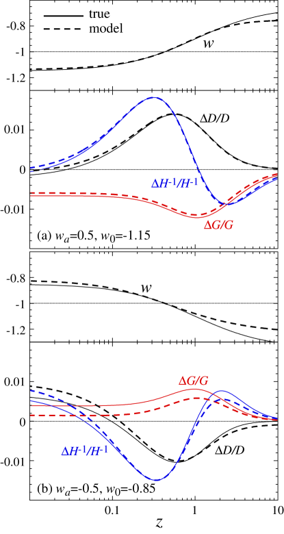
Figure 1: Target versus 2 field model behavior of $w$ and the dark energy observables relative to a fiducial $\Lambda$ model (dotted line, see text). Even in this nearly worst case scenario where $w$ crosses the phantom divide near the pivot point $a\sim 3/4$ or $z\sim 0.3$, the model reproduces the observables to $0.1\%$ accuracy for $w_{a}>0$ and only a factor of a few larger for $w_{a}<0$.

To complete the modelling we match the physical energy density (i.e. not relative to critical) at the normalization epoch $a_{n}=3/4$. To scale the dark energy density of the target dark energy model Eqn. (5) we write $\rho_{\rm DE}(a_{n})=\Omega_{\rm DE}\rho_{\rm crit}g_{\rm DE}$ where

$$g_{\rm DE} =a_{n}^{-3(1+w_{0}+w_{a})}e^{-3(1-a_{n})w_{a}}$$ (17)

and analogously introduce

$$g_{\pm}=a_{n}^{-3(1+w_{\pm})}\,.$$ (18)

Thus given a target model with an energy density relative to critical of $\Omega_{\rm DE}$ and Hubble constant parameterized by $H_{0}=100h$km s^-1 Mpc^-1, the 2 field model has an effective Hubble constant $h_{\rm e}$

$$\left({h_{\rm e}\over h}\right)^{2} =\Omega_{\rm DE}{g_{\rm DE}}\left({1+\delta_{n}\over 2g_{+}}+{1-\delta_{n}\over 2g_{-}}\right)+1-\Omega_{\rm DE}$$ (19)

and density relative to critical defined by that Hubble constant of

$$\Omega_{\pm} =\Omega_{\rm DE}g_{\rm DE}{1\pm\delta_{n}\over 2g_{\pm}}\left({h_{\rm e}\over h}\right)^{-2}\,.$$ (20)

Although this construction is completely phenomenological and hence physically contrived, the general point is that once a close matching of $w(a)$ to some target has been achieved with multiple scalar fields, the scalar field dynamics will make the predictions in both the smooth and clustered regimes robust to reparameterization.

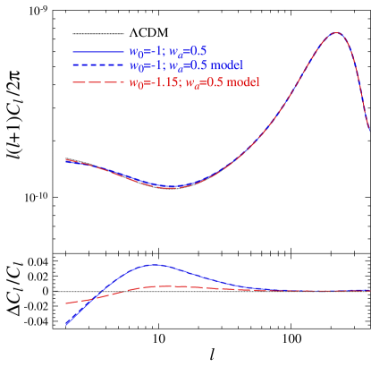
Figure 2: Model predictions for the CMB anisotropy power spectrum relative to a fiducial $\Lambda$CDM model. For models that do not cross the phantom divide, e.g. $w_{0}=-1$, $w=0.5$, the 2 field model matches the single field predictions to $0.1\%$. For crossing models that mimic a cosmological constant by having $w_{n}\approx-1$, e.g. $w_{0}=-1.15$, $w=0.5$, the deviations are essentially indistinguishable.

IV Discussion

In Fig. 1 we show examples of the performance of the model on the dark energy observables of comoving distance $D(z)$, Hubble parameter $H(z)$ and linear growth rate $G(z)$ in the smooth dark energy regime (see Eqn. 4) for strong variations in the equation of state $w_{a}=\pm 0.5$. To better show the relevant performance we choose $w_{0}$ such that $w_{n}\approx-1$ and plot the observables relative to a nearly degenerate fiducial $\Lambda$ model of $\Omega_{\rm DE}=1-\Omega_{m}=0.74$ and $h=0.735$ which is a good fit to the current CMB data. In all cases we adjust the $\Omega_{\rm DE}$ of the target model to match the comoving angular diameter distance to recombination and hence the CMB peak results. Note that for $w_{a}>0$, despite a mismatch in $w$ at very high redshift, all observables as a function of redshift are modeled to the $0.1\%$ level. The performance for $w_{a}<0$ is somewhat worse but never exceeds a few times this level. Thus the two field model will remain an adequate parameterization until the statistical and systematic errors in the dark energy observable measurements reaches the sub $1\%$ level. Mismatches at this point merely reflect the unavoidable fact that higher order derivatives in $w(a)$ produce observable effects and our target constant $w_{a}$ model is itself inadequate. Even in this regime the 2 field model can be useful since the parameter $\epsilon_{n}$ can be used to marginalize or probe the second derivative.

The two field model allows one to also calculate the CMB anisotropy. For a case with no crossing of the divide, e.g. $w_{a}=0.5$, $w_{0}=-1$, the single field model with the exact $w(a)$ matches the 2 field model with the approximate $w(a)$ to $\sim 0.1\%$, in particular at the low multipoles of the ISW effect (see Fig. 2). In addition to the adequate matching of $w(a)$, this indistinguishability is a consequence of setting all of the sound speeds to $c_{e}=1$. Aside from $w(a)$ the remaining degrees of freedom in a dark energy model involve the transition scale between the smooth and clustered regimes. We also show the predictions for a model that does cross the phantom divide $w_{a}=0.5$, $w_{0}=-1.15$. As this model has an equation of state at the normalization point of $w_{n}=-1.025$, it predicts even smaller deviations from the fiducial $w=-1$ model with no instabilities in the evolution of the gravitational potential.

The model constructed here permits a self-consistent likelihood analysis of dark energy observables involving both models that cross the phantom divide and those that differ strongly from $\Lambda$ in the pivot $w_{n}$. Although predictions for the former class models differ little from the currently favored smooth cosmological constant case, the confidence level at which the latter can be excluded can be affected by a consistent model of dark energy clustering. A detailed study of the effect on current cosmological constraints is beyond the scope of this Brief Report.

If future observations require an evolutionary crossing of the phantom divide, it will be a good indication that the dark energy contains hidden internal degrees of freedom in its physical structure.

Acknowledgments: We thank C. Armendariz-Picon, S. Carroll, A. Lewis and D. Pogosian for useful discussions. WH was supported by the DOE and the Packard Foundation. This work was begun in the Aspen Center for Physics and completed at the KICP under NSF PHY-0114422.

Note added in proof: After completion of this work, we became aware of related work by Guo et al [astro-ph/0410654]

References

- Seljak et al. (2004) U. Seljak et al., Phys. Rev. D submitted, astro (2004).
- Caldwell (2002) R. Caldwell, Phys. Lett. B 545, 23 (2002), eprint astro-ph/9908168.
- Vikman (2004) A. Vikman, Phys. Rev. D submitted (2004), eprint astro-ph/0407107.
- Caldwell et al. (1998) R. Caldwell, R. Dave, and P. Steinhardt, Phys. Rev. Lett. 80, 1582 (1998), eprint astro-ph/9708069.
- Weller and Lewis (2003) J. Weller and A. M. Lewis, Mon. Not. Roy. Astron. Soc. 346, 987 (2003), eprint astro-ph/0307104.
- Bardeen (1980) J. Bardeen, Phys. Rev. D 22, 1882 (1980).
- Gordon and Hu (2004) C. Gordon and W. Hu, Phys. Rev. D in press, astro (2004), eprint astro-ph/0406496.
- Garriga and Mukhanov (1999) J. Garriga and V. Mukhanov, Phys. Lett. B 458, 219 (1999), eprint hep-th/9904176.
- Hu (1998) W. Hu, Astrophys. J. 506, 485 (1998), eprint astro-ph/9801234.
- Steinhardt et al. (1999) P. Steinhardt, L. Wang, and I. Zlatev, Phys. Rev. D 59, 123504 (1999).