Loop length and magnetic field estimates from oscillations detected during an X-ray flare on AT Mic

Abstract

We analyse oscillations observed in the X-ray light curve of the late-type star AT Mic. The oscillations occurred during flare maximum. We interpret these oscillations as density perturbations in the flare loop. Applying various models derived for the Sun, the loop length and the magnetic field of the flare can be estimated. We find a period of 740 s, and that the models give similar results (within a factor of 2) for the loop length ($\sim 5.4\ 10^{10}~{}{\rm cm}$) and the magnetic field ($\sim 100~{}{\rm G}$). For the first time, an oscillation of a stellar X-ray flare has been observed and results thus obtained for otherwise unobservable physical parameters.

1 Introduction

Oscillations in the solar corona have been observed for many years. Wavelength regimes ranging from hard X-ray right down to radio have been investigated to search for evidence of waves. Periods have been found ranging from 0.02 to 1000 s. Table 1 in [*]aschwanden1999b provides an excellent summary of the different periods that have been found, and an explanation for their existence. Most of these waves have been explained by MHD oscillations in coronal loops. [*]roberts2000 has provided an excellent review of waves and oscillations in the corona.

Many of the observations of waves have been determined from variations in intensity brightness. Recently, however, a huge step forward has been achieved in solar coronal physics due to the high spatial resolution available with the Transition Region and Coronal Explorer (TRACE). The first spatial displacement oscillations have been observed in coronal loops ([Aschwanden et al.1999]). It was suggested that these oscillations were triggered by a disturbance from the core flare site. Various MHD waves were investigated and it was found that a fast kink mode wave provides the best agreement with the observed period of 280$\pm$30s.

One of the most exciting aspects of observing waves in this fashion is that it potentially provides us with the capability of determining the magnetic field in the corona. It is notoriously difficult to measure the magnetic field in the corona. Techniques using the near-infrared emission lines have been successful, but have poor spatial resolution. Most frequently, indirect methods are used such as the extrapolations of the coronal magnetic field from the photospheric magnetic field that can be measured using Zeeman splitting. [*]nakariakov2001 made use of the flare-related spatial oscillations sometimes observed when a flare occurs, to determine the magnetic field. They assume that the oscillation is due to a global standing kink wave, and hence the magnetic field is related to the period of the oscillation, the density of the loop, and the length of the loop. In the case of [*]nakariakov2001 they found the magnetic field to be 13$\pm$9G. The errors on this are large due to errors on the determination of density, loop length and period. [*]schrijver2000 suggest that the oscillations are due to a sudden displacement of the magnetic field at the surface which causes an oscillatory relaxation of the field. Recent work by [*]nakariakov2004 suggests that the oscillations are second standing harmonics of acoustic waves tied to the loop length. The model gives a relationship between the oscillation period, the loop length and the average plasma temperature, all of which can be independently observed on the Sun.

Waves are observed across the electromagnetic spectrum on the Sun. However, observations on other stars are rare. One reason for this is that on the Sun, we have the spatial resolution to zoom in on small regions. For example, the transverse TRACE loops that have been observed are away from the main flare site, and hence have lower emission measure. Analysing an X-ray light-curve, for example, would be unlikely to provide evidence of waves if the emission was averaged over the whole Sun. Oscillations have been observed for optical stellar flares (e.g., [Mathioudakis et al.2003] and [Mullan et al.1992]). [*]mathioudakis2003 found a period of 220 s in the decay phase of a white-light flare on the RS CVn binary II Peg. Using this they determine a magnetic field of 1200 G. [*]mullan1992 again found oscillations in X-ray active red dwarfs. They compared their observations to the possibility that they were observing p-modes. On the Sun p-modes give rise to 5-minute oscillations on the surface. They concluded that p-modes could not produce the amplitudes they observed and that it must be coronal oscillations, which have, until now, not been observed.

In this work we observe for the first time an oscillation in the corona of AT Mic. We measure the periodicity, and hence determine the magnetic field. This is the first observation of an X-ray oscillation during a stellar flare.

2 Target

AT Mic (GJ 799A/B) is an M-type binary dwarf, with both stars of the same spectral type (dM4.5e+dM4.5e). Both components of the binary flare frequently. The radius of AT Mic given by [*]lim1987 is $2.6~{}10^{10}~{}{\rm cm}$, using a stellar distance of 8.14 pc ([Gliese & Jahreiss1991]). Correcting for the newer value for the distance from HIPPARCOS ($10.2\pm 0.5~{}{\rm pc}$, [Perryman et al.1997]), using that the stellar radius is proportional to the stellar distance for a given luminosity and spectral class, we obtain a stellar radius of $r_{\star}=3.3~{}10^{10}~{}{\rm cm}=0.47~{}r_{\sun}$. The mass of AT Mic given by [*]lim1987 is $m_{\star}=0.4~{}m_{\sun}$.

3 Observation

For our analysis we used the XMM-Newton observations of AT Mic on 16 October 2000 during revolution 156. [*]raassen2003 have analysed this data spectroscopically, obtaining elemental abundances, temperatures, densities and emission measures, while a comparative flare analysis between X-ray and simultaneously observed ultraviolet emissions can be found in [*]mitra-kraev2004. Here, we solely used the 0.2–12 keV X-ray data from the pn-European Photon Imaging Camera (EPIC-pn).

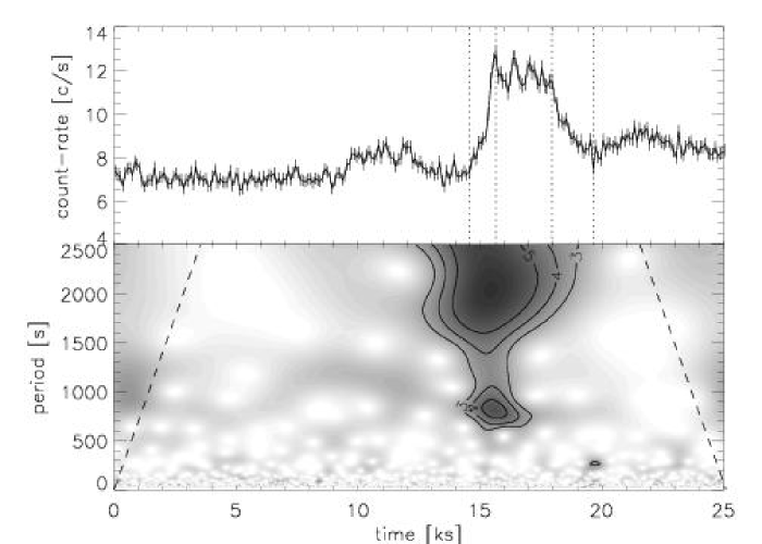
Figure 1: The light curve and wavelet coefficients of AT Mic. The observation started on 2000-10-16 at 00:42:00 h and lasted for 25’100 s ($\sim$ 7 h). The upper panel shows the observed light curve, binned up to 100 s. The vertical dashed lines indicate the start and end of the rise and decay phase of the flare. The lower panel shows the absolute values of a section of the corresponding wavelet coefficients (see main text) divided by their standard deviation. The 3, 4 and 5 $\sigma$ significance contour lines are drawn. The two dashed lines mark the border of the cone of influence. A local maximum is clearly seen with a period of around 740 s during the flare peak.

Figure 1 shows the AT Mic light curve. The observation started at 00:42:00 and lasted for 25.1 ks ($\sim$ 7 h). There is one large flare, starting $\sim$ 4 h into the observation, increasing the count-rate from flare onset to flare peak by a factor of 1.7, and lasting for 1 h 25 min. It shows a steep rise (rise time $\tau_{r}=1100~{}{\rm s}$) and decay (decay time $\tau_{d}=1700~{}{\rm s}$). There is an extended peak to this flare, which shows clear oscillatory behaviour. The amplitude of the oscillation is around 16%. Applying multi-temperature fitting, [*]raassen2003 obtain a mean flare temperature $T=24\pm 4~{}{\rm MK}$ and a quiescent temperature $T_{q}=13\pm 1~{}{\rm MK}$, and from the O vii line ratio a flare and quiescent electron density of $n=4^{+5}_{-3}~{}10^{10}~{}{\rm cm}^{-3}$ and $n_{q}=1.9\pm 1.5~{}10^{10}~{}{\rm cm}^{-3}$, respectively. The total flare and quiescent emission measures are $EM=(19.5\pm 0.8)10^{51}~{}{\rm cm^{-3}}$ and $EM_{q}=(12.2\pm 0.5)10^{51}~{}{\rm cm^{-3}}$.

One of the reasons why we concentrated on this observation is that following the rise phase of the flare there was a period of approximately 40 minutes when the light curve stayed at a high intensity level and showed strong oscillations. The oscillatory activity can be clearly seen by eye (see Fig. 1), and shows behaviour suggestive of damping. This character is much different from solar flares where the flare reaches a peak rapidly, followed by a slow decay. For example, [*]svestka shows solar flare light curves and a flat top is not seen. An alternative to oscillations for this flare is that repeated and rapid flaring is occurring. We do not consider this option in this paper, and assume for our analysis that we are observing a coronal oscillation. The purpose of our analysis is to determine through wavelet analysis the period and amplitude of the oscillation. We determine the magnetic field and loop length of the coronal loop assuming that the oscillation is due to an acoustic wave. As a validity check the value of loop length was compared to the value determined from a radiative cooling model.

4 Results

4.1 Oscillation during flare maximum

To investigate periodicities during the observation, we applied a continuous wavelet transformation to the 10s-binned-data, using a Morlet wavelet (see, e.g., [Torrence & Compo1998]). The wavelet coefficients with the lowest periods are displayed in Fig. 1. The flare oscillation is picked up with a 5$\sigma$ significance level. The local maximum with the shortest period and a significance of more than 5$\sigma$ is simultaneous with the flare top and identifies the oscillation, which, at the local maximum, has a period of $P=740~{}{\rm s}$ . The period interval where the wavelet coefficients have a significance of 5$\sigma$ or more, is [730,920] s.

4.2 Loop length from oscillation

Interpreting these oscillations as the second spatial harmonics of an acoustic wave within the flare ([Nakariakov et al.2004]), we can then determine the flare loop length from

$$L\ [{\rm Mm}]\approx\frac{1}{6.7}\cdot P\ [{\rm s}]\cdot\sqrt{T\ [{\rm MK}]}.$$ (1)

Inserting the above obtained period $P=740~{}{\rm s}$ and a flare temperature $T=24~{}{\rm MK}$, we obtain a loop length $L=5.4~{}10^{10}~{}{\rm cm}$. Note that the temperature carries a $1\sigma$ error of $\sim 16\%$, therefore the error of $L$ is at least 8% ($\Delta L>0.5~{}10^{10}~{}{\rm cm}$). It is not straightforward to calculate the corresponding $1\sigma$ error of $P$. With these numbers, the inferred speed of sound is $c_{s}=L/P\approx 730~{}{\rm km/s}$.

4.3 Loop length from radiative cooling times

The loop length can also (and independently of any oscillation) be estimated from rising and cooling times obtained from the temporal shape of the flare, applying a flare heating/cooling model (see, e.g., [Cargill et al.1995]). We follow the approach by [*]hawley1995 who investigated a flare on AD Leo observed in the extreme ultraviolet. The shape of this flare is very similar to our flare on AT Mic, but roughly 10 times larger (in duration as well as in the increase of the count rate). It also shows a flat top with a possible oscillation. The flare loop energy equation for the spatial average is given by

$$\frac{3}{2}\ \dot{p}=Q-R,$$ (2)

with $Q$ the volumetric flare heating rate, $R$ the optically thin cooling rate and $\dot{p}$ the time rate change of the loop pressure. During the rise phase, strong evaporative heating is dominant ($Q\gg R$), while the decay phase is dominated by radiative cooling and strong condensation ($R\gg Q$). At the loop top, there is an equilibrium ($R=Q$). The loop length can be derived as

$$L=\frac{1500}{\left(1-x_{d}^{1.58}\right)^{4/7}}\cdot\tau_{d}^{4/7}\cdot\tau_{r}^{3/7}\cdot T^{1/2},$$ (3)

where $\tau_{r}$ is the rise time, $\tau_{d}$ the flare decay time (indicated in Fig. 1 with the vertical dotted lines), $T$ the apex flare temperature and $x_{d}^{2}=c_{d}/c_{max}$, with $c_{max}$ the peak count rate and $c_{d}$ the count rate at the end of the flare. Inserting these values, the loop length becomes $L=2.3~{}10^{10}~{}{\rm cm}$, which is about a factor of 2 smaller that the loop length inferred from the oscillation.

4.4 Determination of the Magnetic field

Interpreting the oscillations in terms of global standing kink waves, [*]nakariakov2001 derive a relation for the magnetic field

$$B=\sqrt{8\pi}\ \frac{L}{P}\ \sqrt{\rho\left(1+\frac{\rho_{ext}}{\rho}\right)},$$ (4)

with $\rho$ the mass density inside, and $\rho_{ext}$ the mass density outside the loop. Note that there is a correction factor of 0.64 in the equation as presented by [*]nakariakov2001 ([Mathioudakis et al.2003]). We can simplify Eq. (4) by inserting Eq. (1) and using $\rho=m_{p}\cdot n$ and $\rho_{ext}=m_{p}\cdot n_{q}$, with $m_{p}$ the proton mass. Then, the magnetic field is given by

$$B=\frac{\sqrt{8\pi}}{6.7}\cdot 10^{5}\cdot\sqrt{Tm_{p}n\left(1+\frac{n_{q}}{n}\right)}.$$ (5)

Inserting the temperature and densities from the spectroscopy results, we obtain a magnetic field of $B=115\pm 56~{}{\rm G}$. Note that the large error is resulting mainly from the density uncertainty. Using the loop length from the radiative cooling approach (Sect. 4.3) and Eq. 4, the magnetic field is $B\approx 50~{}{\rm G}$.

4.5 Pressure balance

To maintain stable flare loops, the gas pressure of the evaporated plasma must be smaller than the magnetic pressure

$$2nkT\leq\frac{B^{2}}{8\pi}.$$ (6)

Knowing the flare density and temperature, we get a lower limit for the magnetic field $B>80\pm 60~{}{\rm G}$. Again, there is a large error because of the large uncertainty for the density. [*]shibata2002 assume pressure balance and give equations for $B(EM,n_{q},T)$ and $L(EM,n_{q},T)$ (their Eqs 7a,b). Using these relations, we obtain a magnetic field of $B=70\pm 40~{}{\rm G}$ and a loop length of $L=(2.8\pm 1.7)\ 10^{10}~{}{\rm cm}$.

5 Discussion and Conclusions

We have used three different approaches to determine the loop length of the AT Mic flare and two different approaches for the magnetic field. The loop length derived in Sect. 4.2 from the flare oscillation is the largest with $L=5.4\cdot 10^{10}~{}{\rm cm}$, while the loop length derived from radiative cooling times (Sect. 4.3) is somewhat smaller by roughly a factor of 2, $L=2.3~{}10^{10}~{}{\rm cm}$. The loop length derived from pressure balance (Sect. 4.5) is similar to the latter one, $L=(2.8\pm 1.7)\ 10^{10}~{}{\rm cm}$. The loop length derived by assuming that the variations seen are due to oscillations is a factor of 2 different to the loop length determined by more usual methods. Considering the assumptions that have to be made, this is good agreement, and gives us confidence that we are, for the first time, observing a stellar coronal loop oscillating. The magnetic field ranges from 50 G (radiative cooling) to 115$\pm$56 G (oscillation), with the value from pressure balance in between with 70$\pm$40 G. Again, these three values are all consistent.

This was the first time that an oscillation during flare peak was observed in X-rays in a stellar flare and flare loop length and magnetic field derived from it. The values are consistent with other flare models.