Random-Walk Statistics and the Spherical Harmonic Representation of CMB Maps

Abstract

We investigate the properties of the (complex) coefficients obtained in a spherical harmonic representation of temperature maps of the cosmic microwave background (CMB). We study the effect of the coefficient phase only, as well as the combined effects of phase and amplitude. The method used to check for anomalies is to construct a “random walk” trajectory in the complex plane where the step length and direction are given by the amplitude and phase (respectively) of the harmonic coefficient. If the fluctuations comprise a homogeneous and isotropic Gaussian random field on the sky, the path so obtained should be a classical “Rayleigh flight” with very well known statistical properties. We illustrate the use of this random-walk representation by using the net walk length as a test statistic, and apply the method to the coefficients obtained from a Wilkinson Microwave Anisotropy Probe (WMAP) preliminary sky temperature map.

1 Introduction

The process of gravitational instability initiated by small primordial density perturbations is a vital ingredient of cosmological models that attempt to explain how galaxies and large-scale structure formed in the Universe. In the standard cosmological models, a period of accelerated expansion (“inflation”) generated density fluctuations with simple statistical properties through quantum processes (Starobinsky 1979, 1980, 1982; Guth 1981; Guth & Pi 1982; Albrecht & Steinhardt 1982; Linde 1982). In this scenario the primordial density field is assumed to form a statistically homogenous and isotropic Gaussian Random Field (GRF). Over years of observational scrutiny this paradigm has strengthened its hold in the minds of cosmologists and has survived many tests, culminating in those furnished by the Wilkinson Microwave Anisotropy Probe (WMAP; Bennett et al. 2003; Hinshaw et al 2003).

Since the release of the first (preliminary) WMAP data set it has been subjected to a number of detailed independent analyses that have revealed some surprising features. Eriksen et al. (2004) have pointed out the existence of a North-South asymmetry suggesting that the cosmic microwave background (CMB) revealed by the WMAP data is not statistically homogeneous over the celestial sphere. This is consistent with the results of Coles et al. (2004) who found evidence for phase correlations in the WMAP data; see also Hajian & Souradeep (2003) and Hajian, Souradeep & Cornish (2004). The low–order multipoles of the CMB also display some peculiarities (de Oliveira-Costa et al. 2004a; Efstathiou 2004). Vielva et al. (2004) found significant non–Gaussian behaviour in a wavelet analysis of the same data, as did Chiang et al. (2004), Larson & Wandelt (2004) and Park (2004). Other analyses of the statistical properties of the WMAP have yielded results consistent with the standard form of fluctuation statistics (Komatsu et al. 2003; Colley & Gott 2003). These unusual properties may well be generated by residual foreground contamination (Banday et al. 2003; Naselsky et al. 2003; de Oliveira-Costa et al. 2004; Dineen & Coles 2004) or other systematic effects, but may also provide the first hints of physics beyond the standard cosmological model.

In order to tap the rich source of information provided by future CMB maps it is important to devise as many independent statistical methods as possible to detect, isolate and diagnose the various possible causes of departures from standard statistics. One particularly fruitful approach is to look at the behaviour of the complex coefficients that arise in a spherical harmonic analysis of CMB maps. Chiang et al. (2004), Chiang, Naselsky & Coles (2004), and Coles et al. (2004) have focussed on the phases of these coefficients on the grounds that a property of a statistically homogenous and isotropic GRF is that these phases are random. Phases can also be use to test for the presence of primordial magnetic fields (Chen et al. 2004; Naselsky et al. 2004) or evidence of non-trivial topology (Dineen, Rocha & Coles 2004). In this paper we suggest an extension of this idea which involves viewing the entire set of harmonics (both amplitude and phase) in the complex plane.

We describe the basic harmonic description in the next Section. In Section 3 we show how to represent the spherical harmonics as random-walks in the complex plane and give some simple analytic results. We apply the idea to the preliminary WMAP 1-year data in Section 4 and briefly discuss the results in Section 5.

2 Spherical Harmonics and Gaussian Fluctuations

We can describe the distribution of fluctuations in the microwave background over the celestial sphere using a sum over a set of spherical harmonics:

$$\Delta(\theta,\phi)=\frac{T(\theta,\phi)-\bar{T}}{\bar{T}}=\sum_{l=1}^{\infty}\sum_{m=-l}^{m=+l}a_{l,m}Y_{lm}(\theta,\phi).$$ (1)

Here $\Delta(\theta,\phi)$ is the departure of the temperature from the average at angular position $(\theta,\phi)$ on the celestial sphere in some coordinate system, usually galactic. The $Y_{lm}(\theta,\phi)$ are spherical harmonic functions which we define in terms of the Legendre polynomials $P_{lm}$ using

$$Y_{lm}(\theta,\phi)=(-1)^{m}\sqrt{\frac{(2l+1)(l-m)!}{4\pi(l+m)!}}P_{lm}(\cos\theta){\rm e}^{im\phi},$$ (2)

i.e. we use the Condon-Shortley phase convention. In Equation (1), the $a_{l,m}$ are complex coefficients which can be written

$$a_{l,m}=x_{l,m}+iy_{l,m}=|a_{l,m}|\exp[i\phi_{l,m}].$$ (3)

Note that, since $\Delta$ is real, the definitions (2) & (3) requires the following relations between the real and imaginary parts of the $a_{l,m}$: if $m$ is odd then

$$x_{l,m}=\Re(a_{l,m}) = -\Re(a_{l,-m})=-x_{l,-m},$$

$$y_{l,m}=\Im(a_{l,m}) = \Im(a_{l,-m})=y_{l,-m};$$ (4)

while if $m$ is even

$$x_{l,m}=\Re(a_{l,m}) = \Re(a_{l,-m})=x_{l,-m},$$

$$y_{l,m}=\Im(a_{l,m}) = -\Im(a_{l,-m})=y_{l,-m};$$ (5)

and if $m$ is zero then

$$\Im(a_{l,m})=y_{l,0}=0.$$ (6)

From this it is clear that the $m=0$ mode always has zero phase, and there are consequently only $l$ independent phase angles describing the harmonic modes at a given $l$. Without loss of information we can therefore restrict our analysis to $m\geq 0$.

If the primordial density fluctuations form a Gaussian random field in space the temperature variations induced across the sky form a Gaussian random field over the celestial sphere. This means that

$$\langle a_{l,m}a_{l^{\prime},m^{\prime}}^{*}\rangle=C_{l}\delta_{ll^{\prime}}\delta_{mm^{\prime}},$$ (7)

where $C_{l}$ is the angular power spectrum, the subject of much scrutiny in the context of the cosmic microwave background (e.g. Hinshaw et al. 2003), and $\delta_{xx^{\prime}}$ is the Kronecker delta function. Since the phases are random, the stochastic properties of a statistically homogeneous and isotropic Gaussian random field are fully specified by the $C_{l}$, which determines the variance of the real and imaginary parts of $a_{l,m}$ both of which are Gaussian:

$$\sigma^{2}(x_{l,m})=\sigma^{2}(y_{l,m})=\sigma_{l}^{2}=\frac{1}{2}C_{l}.$$ (8)

3 Random Walks in Harmonic Space

To begin with, we concentrate on a simple measure based on the distribution of total displacements. Consider a particular value of $l$. The set of values $\{{\bf a_{l,m}}\}$ can be thought of as steps in a random walk in the complex plane, a structure which can be easily visualized and which has well-known statistical properties.

The simplest statistic one can think of to describe the set $\{{\bf a_{l,m}}\}$ is the net displacement of a random walk corresponding to the spherical harmonic mode $l$, i.e.

$${\bf R_{l}}\equiv(X_{l},Y_{l})=\sum_{m>0}{\bf a_{l,m}},$$ (9)

where the vector ${\bf a_{l,m}}\equiv(x_{l,m},y_{l,m})$ and the random walk has an origin at $a_{l,0}$ (which is always on the $x$-axis). The length of each step $a_{l,m}=|{\bf a_{l,m}}|$ is the usual spherical harmonic coefficient described in the previous section and defined by equation (1). If the initial fluctuations are Gaussian then the two components of each displacement are independently normal with zero mean and the same variance (8). Each step then has a Rayleigh distribution so that the probability density for $a_{l,m}$ to be in the range $(a,a+da)$ is

$$p(a)=\frac{a}{\sigma_{l}^{2}}\exp\left(-\frac{a^{2}}{2\sigma_{l}^{2}}\right).$$ (10)

This is a particularly simple example of a random walk (McCrea & Whipple 1940; Chandrasekhar 1943; Hughes 1995). Since the displacements in $x$ and $y$ are independently Gaussian the next displacement after $l$ steps is itself Gaussian with variance $l\sigma_{l}^{2}$. The total displacement $R_{l}$ is given by

$$R_{l}^{2}=\left(X_{l}^{2}+Y_{l}^{2}\right).$$ (11)

The probability density of $|R_{l}|$ to be in the range $(r,r+dr)$ is then itself a Rayleigh distribution of the form

$$p_{l}(r)=\frac{r}{l\sigma_{l}^{2}}\exp\left(-\frac{r^{2}}{2l\sigma_{l}^{2}}\right).$$ (12)

The result (12) only obtains if the steps of the random walk are independent and Gaussian. If the distribution of the individual steps is non-Gaussian, but the steps are independent, then the result (11) will be true for large $l$ by virtue of the Central Limit Theorem. Exact results for finite $l$ for example non-Gaussian distributions are given by Hughes (1995).

A slightly different approach is to keep each step length constant. The simplest way of doing this is to define

$${\bf\hat{R}_{l}}=\sum_{m>0}\frac{{\bf a_{l,m}}}{|{\bf a_{l,m}}|}=\sum_{m>0}{\bf\hat{a}_{l,m}},$$ (13)

so that each step is of unit length but in a random direction. This is precisely the problem posed in a famous letter by Pearson (1905) and answered one week later by Rayleigh (1905). In the limit of large numbers of steps the result maps into the previous result (12) with $\sigma_{l}^{2}=1$ by virtue of the Central Limit Theorem. For finite values of $l$ there is also an exact result which can be derived in integral form using a method based on characteristic functions (Hughes 1995). The result is that the probability density for ${\bf\hat{R_{l}}}$ to be in the range $r,r+dr$ is

$$q_{l}(r)=r\int_{0}^{\infty}uJ_{0}(ur)[J_{0}(u)]^{l}du.$$ (14)

The integral is only convergent for $l>2$ but for $l=1$ or $l=2$ straightforward alternative expressions are available (Hughes 1995).

One can use this distribution to test for randomness of the phase angles without regard to the amplitudes. To see how this works, consider the following simple model of phase correlations. Following Watts, Coles & Melott (2003), Suppose that the phase difference between adjacent modes has a preferred angle, as modelled by the relation

$${\bf\hat{a}_{l,m}}={\bf\hat{a}_{l,m+1}}\cos\theta-{\bf u_{l,m+1}}.$$ (15)

Here $u_{l,m}$ is a random variable with $|u_{l,m}|=|\sin\theta|$, $\langle{\bf u_{l,m}}\rangle=0$ and ${\bf u_{l,m}}\cdot{\bf\hat{a}_{l,m}}=0$, to keep the step length equal to unity. In this model

$$\langle{\bf\hat{a}_{l,m}}\cdot{\bf\hat{a}_{l,m+n}}\rangle=\langle{\bf\hat{a}_{l,m+1}}\cdot{\bf\hat{a}_{l,m}}\rangle\cos\theta=\cos^{n}\theta.$$ (16)

Hence

$$\langle R_{l}^{2}\rangle=l+2\sum_{n>m}\langle{\bf\hat{a}_{l,m}}\cdot{\bf\hat{a}_{l,m+n}}\rangle,$$ (17)

which is

$$\langle R_{l}^{2}\rangle=N+2\sum_{n=2}^{l}\sum_{m=1}^{n-1}\cos^{n-m}\theta.$$ (18)

Using the properties of a geometric series this can be seen to be

$$\langle R_{l}^{2}\rangle=l\left(\frac{1+\cos\theta}{1-\cos\theta}\right)=\frac{l}{\xi^{2}},$$ (19)

compared with the simple $\langle R_{l}^{2}\rangle=l$ which obtains if the phases are random. The distribution of total displacements therefore encodes information about phase correlations in the form of a “persistence length”, $\xi$. The distribution of $R_{l}$ therefore encodes information about phase correlations: if there is no preferred direction, $\cos\theta=0$ and the result reduces to the case of a purely random walk with $\xi=1$. Non-zero values of $\cos\theta$ will alter the mean square displacement relative to this case: it can be either larger if $\cos\theta$ is positive and steps tend to occur in the same direction in the complex plane ($\xi>1$), or smaller if $\xi<1$.

So far we have concentrated on fixed $l$ with a random walk as a function of $m$. We could instead have fixed $m$ and considered a random walk as a function of $l$. Or indeed randomly selected $N$ values of $l$ and $m$. In either case the results above still stand except with $\sigma_{l}^{2}$ replaced by an average over all the modes considered:

$$\sigma^{2}=\frac{1}{N}\sum_{l,m}\sigma_{l,m}^{2}.$$ (20)

We do not consider this case any further in this paper.

4 Application to the WMAP 1 yr Data

There are many possible ways of using the properties of a random walk to test the hypothesis that the CMB temperature fluctuations are drawn from a statistically homogeneous and isotropic Gaussian random field on the sky could be furnished by comparing the empirical distribution of harmonic random flights with the form (12). This requires an estimate of $\sigma_{l}^{2}$. This can either be made using the same data or by assuming a given form for $C_{l}$, in which case the resulting test would be of a composite hypothesis that the fluctuations constitute a Gaussian random field with a particular spectrum. For large $l$ this is can be done straightforwardly, but for smaller values the sampling distribution of $R_{l}$ will differ significantly from (12) because of the uncertainty in population variance from a small sample of $a_{lm}$. This is the so-called “cosmic variance” problem.

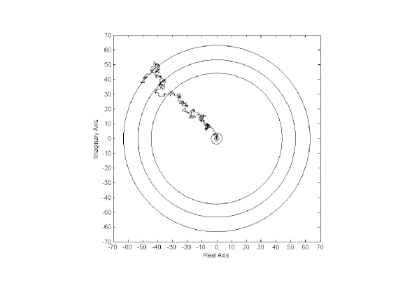
Figure 1: The random walk performed by the spherical harmonic coefficients for $l=532$, statistically the mode that displays the greatest departure from that expected under the null hypothesis. The outer circles correspond to 99.9, 99 and 95 per cent upper confidence limits s (from outer to inner); the inner circles are the corresponding lower limits, though the 99.9 per cent lower limit is too small to see.

In practice the most convenient way to assess the significance of departures from the relevant distribution would be to perform Monte Carlo experiments of the null hypothesis. For statistical measures more complicated than the net displacement, the best way to set up a statistical test is to use Monte-Carlo re-orderings of the individual steps to establish the confidence level of any departure from Gaussianity. This also enables one to incorporate such complications as galactic cuts.

The WMAP team released an Internal Linear Combination (ILC) map that combined five original frequency band maps in such a way to maintain unit response to the CMB whilst minimising foreground contamination. The construction of this map is described in detail in Bennett et al. (2003). The weighted map is produced by minimizing the variance of the temperature scale such that the weights add to one. To further improve the result, the inner Galactic plane is divided into 11 separate regions and weights determined separately. This takes account of the spatial variations in the foreground properties. Thus, the final combined map does not rely on models of foreground emission and therefore any systematic or calibration errors of other experiments do not enter the problem. The final map covers the full-sky and the idea is that it should represent only the CMB signal. Following the release of the WMAP 1 yr data Tegmark, Oliveira-Costa & Hamilton (2003; TOH) produced a cleaned CMB map. They argued that their version contained less contamination outside the Galactic plane compared with the ILC map produced by the WMAP team.

The ILC map is not intended for statistical analysis but in any case represents a useful “straw man” for testing statistical techniques for robustness. To this end, we analyzed the behaviour of the random-walks representing spherical harmonic from $l=1$ to $l=600$ in the WMAP ILC. Similar results are obtained for the TOH map so we do not discuss the TOH map here. For both variable-length (9) and unit-length (13) versions of the random-walk we generated 100000 Monte Carlo skies assuming Gaussian statistics. These were used to form a distribution of $|{\bf R_{l}}|$ (or $|{\bf\hat{R}_{l}}|$) over the ensemble of randomly-generated skies. A rejection of the null hypothesis (of stationary Gaussianity) at the $\alpha$ per cent level occurs when the measured value of the test statistic lies outstide the range occupied by $\alpha$ per cent of the random skies. The results we obtained are summarized in Table 1.

confidence level	95	99	99.9
unit length	33	6	2
variable length	20	4	1
null	30	6	0.6

Table 1: Results for random-walks with variable step-length and unit step-length for the WMAP ILC data. The columns show the number of $l$-modes for which the test statistic lies outside the $\alpha$ percent confidence limit for the Monte Carlo skies. The final row shows the number of modes that would be expected, on average, to lie outside this range if the null hypothesis were true.

The results show that this simple test does not strongly falsify the null hypothesis, which is not surprising given the simplicity of the measure we have used. The number of modes outside the accepted range is close to that which would be expected if the null hypothesis were true. Notice that slightly more modes show up in the unit length case than in the other, perhaps indicating that the phase correlations that are known to exist in this data (Chiang et al. 2004) are masked if amplitude information is also included. The most discrepant mode turns out to be $l=532$ in both cases. For interest a plot of the random walk for this case is included as Figure 1.

We can turn these results into limits on the persistence length: if $\xi$. If $\xi\neq 0$ there would be either more observed walks longer than the limits ($\xi>1$) corresponding to the null hypothesis or more shorter ones ($\xi<1$). Assuming the form (12), which should hold for large values of $l$, the current data place rough limits of $0.9<\xi<1.1$.

5 Discussion and Conclusions

We have presented a novel representation of the behaviour of spherical harmonic coefficients obtained in the representation of of CMB temperature maps. Indeed, the main result of this paper is the construction of two-dimensional walks as discussed in Section 3. In order to illustrate the method in the simplest way we performed a simple statistical test on the net displacement of the random walks for different $l$ modes. The results of this analysis do not provide conclusive evidence for departures from a homogeneous and isotropic GRF. For example, two modes are discrepant at 99.9 per cent confidence, compared with the 0.6 expected by chance. In a series of independent random skies with an expectation of 0.6 modes, Poisson statistics give a probability of 88 per cent that less than two modes would be discrepant. The detection of two modes is therefore not an indication of a strong departure from chance.

It is worth noting that the method does not pick out any significant departures at low $l$, which is where the non-parametric tests of Coles et al. (2004) were applied with positive results. This test works better with large numbers of independent $m$ modes. In the simple form presented here it seems less powerful than the phase-mapping technique of Chiang et al. (2003) and Chiang et al. (2004). Whatever forms of non-Gaussianity and/or non-stationarity there are in these data, this very simple test is not sensitive to them.

As we explained above, however, the net displacement of the random walk is a simple but rather crude indication of the properties of the $\{{\bf a_{l,m}}\}$, as it does not take into account the ordering of the individual steps. The possible non-Gaussian behaviour of the set $\{{\bf a_{l,m}}\}$ is encoded not so much in the net displacement but in the shape of the random walk. To put this another way, there are many possible paths with the same net displacement, and these will have different shapes depending on the correlations between step size and direction. Long runs of directed steps or regular features in the observed structure could be manifestations of phase correlation (Coles et al. 2004). For example, the presence of a primordial magnetic field contribution to the CMB fluctuations would result in a correlation between ${\bf a_{l-1,m}}$ and ${\bf a_{l+1,m}}$ at fixed $m$ (Chen et al. 2004). Examples of how similar effects might be produced by foregrounds, galactic cuts and so on are discussed by Naselsky et al. (2005). These phase correlations would manifest themselves in higher-order statistics of the random walk as a function of $l$. It will also be useful, say, to combine random walks as functions of $m$ for different $l$: correlations between the net displacements of such walks would indicate the presence of phase correlations too; see Coles et al. (2004). The graphical representation of the set $\{{\bf a_{l,m}}\}$ in the form illustrated by Figure 1 provides an elegant way of visualizing the behaviour of the harmonic modes and identifying any oddities. These could be quantified using a variety of statistical shape measures: moment of inertia (Rudnick, Beldjenna & Gaspari 1987), fractal dimension, first-passage statistics, shape statistics (e.g. Kuhn & Uson 1982), or any of the methods use to quantify the shape of minimal spanning trees (Barrow, Bhavsar & Sonoda 1985). It would be interesting to try these more sophisticated measures on subsequent releases of the WMAP data.

References

- [Albrecht & Steinhardt 1982] Albrecht A., Steinhardt P. J., 1982, Phys. Rev. Lett., 48, 1220
- [Banday et al. 2003] Banday A.J., Dickinson C., Davies R.D., Davies R.J., Górski K.M. 2003, MNRAS, 345, 897
- [Bardeen et al. 1986] Bardeen J.M., Bond J.R., Kaiser N, Szalay A.S., 1986, ApJ, 304, 15
- [Barrow et al. 1985] Barrow J.D., Bhavsar S.P., Sonoda D.H., 1985, MNRAS, 216, 17
- [Bennett et al. 2003] Bennett C., et al. 2003, ApJS, 148, 1
- [Chandrasekhar 1943] Chandrasekhar S., 1943, Rev. Mod. Phys., 15, 1
- [Chen et al. 2004] Chen G., Mukherjee P., Kahniashvili T., Ratra B., Wang Y., 2004, ApJ, 611, 655
- [Chiang, Naselsky & Coles 2004] Chiang L.-Y., Naselsky P.D., Coles P., 2004, ApJ, 602, L1
- [Chiang et al. 2003] Chiang L.-Y., Naselsky P. D., Verkhodanov O. V., Way M. J., 2003, ApJ, 590, L65
- [Coles et al. 2004] Coles P., Dineen P., Earl J., Wright D., 2004, MNRAS, 350, 989
- [Colley & Gott] Colley W.N., Gott J.R., 2003, MNRAS, 344, 686
- [De Oliveira-Costa et al. 2004a] de Oliveira-Costa A., Tegmark M., Zaldarriaga M., Hamilton A.J.S., 2004, Phys. Rev. D., 69, 063516
- [De Oliveira-Costa et al. 2004b] de Oliveira-Costa A., Tegmark M., Davies R.D., Gutierrez C.M., Lasenby A.N., Rebolo R., Watson R.A., 2004, ApJ, 606, L89
- [Dineen & Coles 2004] Dineen P., Coles P., 2004, MNRAS, 348, 52
- [Dineen et al. 2004] Dineen P., Rocha G., Coles, P., 2005, MNRAS, 358, 1285
- [Efstathiou 2004] Efstathiou G., 2004, MNRAS, 348, 885
- [Eriksen et al. 2004] Eriksen H. K., Hansen F. K., Banday A. J., Gorski K. M., Lilje P. B., 2004, ApJ, 605, 14
- [Guth 1981] Guth A. H., 1981, Phys. Rev. D., 23, 347
- [Guth & Pi 1982] Guth A. H., Pi S.-Y., 1982, Phys. Rev. Lett. 49, 1110
- [Hajian & Souradeep 2003] Hajian A., Souradeep T., 2003, ApJ, 597, L5
- [Hajian, Souradeep & Cornish 2004] Hajian, Souradeep T., Cornish N., 2004, preprint, astro-ph/0406354
- [Hinshaw et al. 2003] Hinshaw G. et al. 2003, ApJ, 148,
- [Hughes 1995] Hughes B.D., 2004, Random Walks and Random Environments. Volume 1: Random Walks. Oxford University Press, Oxford.
- [Komatsu et al. 2003] Komatsu E. et al. 2003, ApJ, 148, 119
- [Kuhn & Uson 1982] Kuhn J.R., Uson J.M., 1982, ApJ, 263, L47
- [Larson & Wandelt 2004] Larson D.L., Wandelt B.D., 2004, ApJ, 613, L85
- [Linde 1982] Linde, A.D., 1982, Phys. Lett. B., 108, 389
- [McCrea & Whipple 1940] McCrea W.H., Whipple F.J.W., 1940, Proc. R. Soc. Edin., 60, 281
- [Naselsky et al. 2004] Naselsky P.D., Chiang L.-Y., Olesen P., Verkhodanov O., 2004, astro-ph/0405181
- [Naselsky, Doroshkevich & Verkhodanov 2003] Naselsky P.D., Doroshkevich A.G., Verkhodanov O., 2003, ApJ, 599, L53
- [Naseksly et al. 2005] Naselsky P.D., Chiang L.-Y., Olesen P., Novikov I., 2005, Phys. Rev. D., submitted, astro-ph/0505011
- [Park 2004] Park, C.-G., 2004, MNRAS, 349, 313
- [Pearson 1905] Pearson K., 1905, Nature, 72, 294
- [Rayleigh 1905] Rayleigh, 1905, Nature, 72, 318
- [Rudnick et al.] Rudnick J., Beldjenna A., Gaspari G., 1987, J. Math. Phys. A, 20, 971
- [Smoot et al. 1992] Smoot G.F. et al. 1992, ApJ, 396, L1
- [Starobinsky 1979] Starobinsky A. A., 1979, Pis’ma Zh. Eksp. Teor. Fiz., 30, 719
- [Starobinsky 1980] Starobinsky A. A., 1980 Phys. Lett. B., 91, 99
- [Starobinsky 1982] Starobinsky A. A., 1982, Phys. Lett. B., 117, 175
- [Tegmark, de Oliveira-Costa & Hamilton 2003] Tegmark M., de Oliveira-Costa A., Hamilton A.J.S., 2003, Phys. Rev. D., 68, 123523
- [Vielva et al. 2004] Vielva P., Martinez-Gonzalez E., Barreiro R.B., Sanz J.L., Cayon L., 2004, ApJ, 609, 22
- [Watts et al. 2003] Watts P.I.R., Coles P., Melott A.L., 2003, ApJ, 589, L61