At what particle energy do extragalactic cosmic rays start to predominate?
Abstract
We have argued (e.g. 1 ) that the well-known ‘ankle’ in the
cosmic ray energy spectrum, at logE (eV) 18.7-19.0, marks
the transition from mainly Galactic sources at lower energies to
mainly extragalactic above. Recently, however, there have been
claims for lower transitional energies, specifically from logE
(eV) 17.0 2 via 3 to 18.0
4 . In our model the ankle arises naturally from the sum of
simple power law-spectra with slopes differing by ; from differential slope for Galactic
particles (near logE = 19) to for extragalactic
sources. In the other models, on the other hand, the ankle is
intrinsic to the extragalactic component alone, and arises from
the shape of the rate of energy loss versus energy for the
(assumed)
protons interacting with the cosmic microwave background (CMB).
Our detailed analysis of the world’s data on the ultra-high energy
spectrum shows that taken together, or separately, the resulting
mean sharpness of the ankle (second difference of the
log(intensityE3) with respect to logE) is consistent
with our ‘mixed’ model. For explanation in terms of extragalactic
particles alone, however, the ankle will be at the wrong energy –
for reasonable production models and of insufficient magnitude if,
as seems likely, there is still a significant fraction of heavy
nuclei at the ankle energy.
I Introduction
A key property of the cosmic radiation is the division between those particles of Galactic origin and those which are extragalactic. It is virtually certain that those below about logE (eV) = 17 are Galactic (G) and that the very highest energy particles are extragalactic (EG), but the energy (E0.5) at which EG starts to dominate is debatable. It is this question that is the subject of this paper.
In every model the Galactic magnetic field progressively loses its trapping power as the rigidity increases so that the mean charge of the detected Galactic particles increases. Ideally, measurements of the mass composition should be possible and these would appear to indicate E0.5 but there is the distinct likelihood of a significant fraction of heavy nuclei in the EG beam.
Here, we start by considering the measured spectral shape and then examine the possibility of an explanation in terms of primary protons. This is followed by an analysis of the mass composition and its relevance to the Galactic/Extragalactic boundary.
II The measured spectral shape
A number of measurements have been made over the years, using increasingly large extensive air shower (EAS) arrays. Our earlier work 1 gave a summary and here we update the analysis. Figure 1 gives the individual spectra. It will be noted that, when the energy range covered is large enough, there is clear evidence for the presence of an ankle. Defining ‘sharpness’ as in related work, (e.g. 5 ), by S = with a bin width of logE = 0.2 – or converted to that value – the values derived by us are as given in Table 1 (references to the individual arrays are given in Ref. 1 ).
A variety of methods have been used to determine the sharpness values including a variation where the regions near the individual ankles (0.2 in logE) are not used in determining the actual ankle position in each case. The result is that there should be no artificial sharpening of the overall ankle (a situation suggested by some, e.g. 6 ).
Figure 2 shows the superimposed spectra normalized to the datum intensity 7 and the ankle-energy. It is evident that the well known large systematic differences in intensity do not occur until beyond the ankle region. Figure 3 shows the combined data – and corresponding uncertainties. The extent to which our simple explanation in terms of the addition of a rapidly falling G-spectrum and a standard (approximately E-2) EG-spectrum fits the data near the ankle is clear. The expectation (sum) has observational uncertainties added to it; their effect is very small.
Returning to the sharpness values, set (3) in Table 1 is probably the safest to use. The mean value is S = where the ‘error’ has been derived from the dispersion of the individual values. The expected value for the ‘intersecting lines’ from G and EG spectra, is S = 0.96 without experimental resolution, falling to 0.90 with the inclusion of noise. Thus, there is consistency.
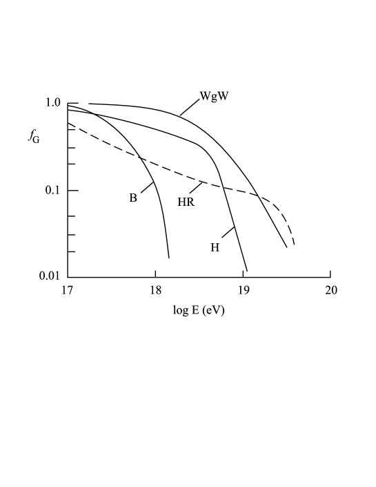
III Models for explaining the spectral shape in the ankle region
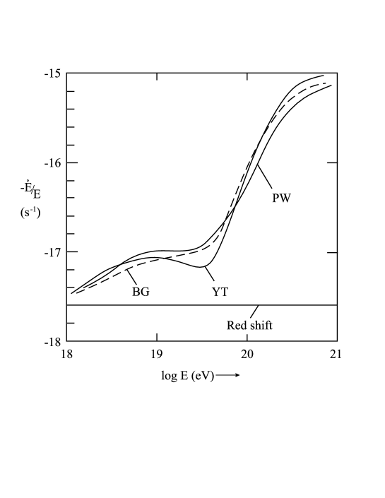
As remarked earlier, the competing models have the Galactic flux reduced to a very low level by the time the ankle is reached and the ankle is formed by the effect of e+e- production on the (assumed) EG proton spectrum. Figure 4 shows the Galactic fraction for the various models, including our own. Figure 5 shows the rate of energy loss for e+e- and pion production from our own calculations 1 and by others 8 ; 9 . If a function of this type is multiplied by an assumed EG injection spectrum then the usual form of EG-proton spectrum is derived; it is evident that there is, indeed, an ankle in the region of log E = 19. Figure 6 shows the multiplying factor for a number of situations, to be described.
It should be pointed out that the use of the factor taken simply as the reciprocal of Figure 5, is for a Euclidian Universe, ie with no expansion and integration for a uniform spatial and temporal distribution of sources out to the Hubble radius. In fact, there will be a number of factors which perturb the simple form of the predicted spectrum, particularly at and below several times log E = 19 (at higher energies the collection volume is local and expansion effects are small). The factors of concern are:
-
1
The limit on red-shift beyond which the spatial density of galaxies – which are potential sources of ultra-high energy cosmic rays (UHECR) – becomes small.
-
2
Scattering of particles, which increases the path length and thereby travel time.
-
3
Possible -dependent production rates (the ‘cosmological increase’ – e.g. 10 )
-
4
The enhanced CMB temperature, and consequent increased energy loss rates for the protons, as increases.
-
5
The stochastic nature of the sources in space and in time.
Concerning 1, there is the immediate problem relating to the actual nature of the sources of UHECR. In order of increasing general activity we have the following approximate densities, in units of number per Gpc3.
| Normal galaxies | 3 out to |
|---|---|
| Colliding galaxies | at small , increasing with |
| Seyfert galaxies | at small , increasing slowly with |
| Quasars | Increasing with , from 2 at to at , then falling 11 |
For protons of log E = 19 the attenuation length in a non-evolving universe is Gpc (ie ) and thus, only for quasars will there be large stochastic effects. The number of quasars in a sphere of radius 0.84 Gpc will be 2 or 3 and at higher energies the stochastic effects will even more serious, however, here we are preoccupied with ‘ankle’-energies (ie log E = 19).
If now we consider the increased energy losses as increases, the collection radius will be smaller than 1.6 Gpc and the stochastic effects for quasars will be larger. When allowance is made for the effect of large scale source density variations due to superclusters (the ‘supercluster-enhancement’, 12 ), voids and ‘great-attractors’, the spectral shape in the region of 1019eV log E = 19 is unlikely to be smooth, if quasars are responsible for the particles. The chance of having the observed ankle and an otherwise smooth spectrum is surely very unlikely.
Seyfert or colliding galaxies seem more likely here, although the temporal variations for Seyfert galaxies (the fact that they are ‘on’ for only about 1% of the time) will be significant.
Turning to factor 2, scattering is no doubt important for 1019 eV protons. The Larmor radius in our usually adopted magnetic field of G 13 is 3 Mpc and the corresponding ‘scattering-horizon’ is about 300 Mpc. This will increase the stochastic fluctuations somewhat, but this effect is unlikely to be large.
As remarked already, Figure 6 shows the factor by which the spectral shape should be multiplied in order to achieve the expected shape. The ‘predictions’ are given for a variety of situations, and can be considered in turn:
-
a
Uniform production model. This is the standard, very approximate, case where it is assumed that there is uniform production everywhere but -dependent losses are ignored. It is taken from the inversion of PW in Figure 5; that derived from the other curves in the Figure would not be very different. It will be noted that there is, indeed, an ankle near log E = 19 in the Euclidian case.
- b
-
c
An estimate for an injection spectrum which has the form E-2 but has an intensity dependence similar to that for radio sources, ie a ‘cosmological increase’ at ‘large’ 10 . The effect of the increase is to raise the intensity of lower energy particles which do not suffer much loss on the CMB.
IV Discussion of the spectral shapes
The first matter to discuss is the actual energy at which the ankle occurs. This depends on the absolute calibration of the energies for which, as has been remarked, there is no agreement. Figure 2 shows the ankle at log E = 18.93 for the Hi-Res 7 normalization; with the AGASA 1 normalization the knee moves up to log E = 19.06. Here we will take log E = 19.0, the mean.
Turning to Figure 6 there is seen to be a wide disparity of shapes but
all have an ankle. It is evident that BG0.33 and PW have ankles at somewhat
too high an energy but, insofar as galaxy-sources of UHECR almost certainly
extend further than this cannot be regarded as fatal for the EG-model.
For PW, the maximum sharpness is:
S, i.e. not inconsistent with observation, although, as
remarked, the energy value is high and the physics is suspect.
For the more likely case of a -dependent injection rate (eg ‘PJ’) the sharpness is reasonable (S) but the energy at which the maximum occurs, log E18.6, is too low.
Before continuing to examine the relevance of the mass spectrum other considerations are necessary, related to the other factors referred to in section 2. The smoothing introduced by factor 5 in section 2, viz stochastic processes is important. One such relates to the non-uniformity of density of galaxies in the universe. Calculations allowing for the enhanced density of local galaxies in the VIRGO supercluster (‘supercluster enhancement’ 12 ) show a displacement of the patterns in figure 6 to higher energies by a factor log E0.2, thereby taking ‘PW’ even further from ‘the truth’.
An examination of the topology of galaxies as a whole shows the presence of remarkable fluctuations in density on scales even higher than that of superclusters. For example, there is evidence for ‘huge regions of underdensity in both hemispheres’ 15 and there is a 30% reduction to (440 Mpc) in the Southern Hemisphere. The net result for the range of distances corresponding to the ankle (840 Mpc for log E = 19) is that we estimate a standard deviation in log E of about 0.3. Application of a Gaussian with this standard deviation causes a reduction in sharpness by a factor of 0.6. The value for PW then become lower than needed.
The conclusion is, therefore, at this stage, that the position of the ankle allows an explanation in terms of EG particles alone, but that its magnitude is rather low (0.6 compared with a needed 0.9). Furthermore, a cosmological increase in Galactic output – which seems likely on general astrophysical grounds – is not allowable, nor indeed is allowance for -dependent losses, which must be present. The decisive blow against the EG origin of the ankle comes from the mass composition, however, and this aspect will now be examined.
V The mass composition of the particles above logE (eV) = 17
The relevance of the mass composition here is that we have assumed, so far, that at least at energies above log E = 19, the bulk of the EG particles are protons. It has proved notoriously difficult to determine the mass spectrum, largely because of uncertainties in the high energy interaction model to be adopted so far above the (accelerator) energies at which the models can be checked, but some progress has been made.
It would be expected that Galactic particles would be increasingly lost as the particle rigidity increases and, in consequence, that the fraction of heavy nuclei (iron) would continuously increase. An indication of the extent of the Galactic component is therefore tied up with the fraction of the beam which we assume to be composed of such heavy nuclei.
Over the years we have studied this aspect in a number of ways, principally by examining the frequency distribution of depth of shower maximum and by studying the data relating to the ‘Galactic Plane Excess’.
Figure 7 shows the results for , the fraction or iron in the primary beam. The results denoted ‘’ are from the frequency distribution of values as analysed by ourselves 16 ; we prefer this technique to that of using the mean (e.g. 7 ) because of the effect of uncertainties in the nuclear interaction model. In the fluctuation model, the high mass ‘tail’ to the distribution is assumed due to iron and the distribution displaced accordingly. The results from the mean are considered later.
The results marked ‘T’ come from our analyses of the b-distribution in the Inner Galaxy using trajectory calculations for particles accelerated in the Galactic Plane 17 .
We turn now to other estimates, from the mean depth of shower maximum. A useful survey 18 gives the median denoted D in Figure 7; this includes the low values from Hi-Res. (II) which provided the reason for the low cross-over point given earlier. (Figure 4). Also included is the latest AGASA measurement 19 , at log E = 19.3, denoted ‘A’.
It is evident that the new determinations (D and A) are, if anything, somewhat higher than our own, particularly above log E = 18.5, so that our estimate of the Galactic fraction in Figure 4 has a measure of confirmation. The values at log E = 19 can be taken as an example. The overall mean of (Figure 7) is at 0.35 so that, for two components only, Galactic iron and Extragalactic protons, the corresponding Galactic fraction is also 0.35. This can be compared with our ‘need’ of 0.35 for the Hi-RES normalization and 0.42 for AGASA. There is clearly no problem in terms of consistency. However, there is an important implication for the expected sharpness, as will now be described.
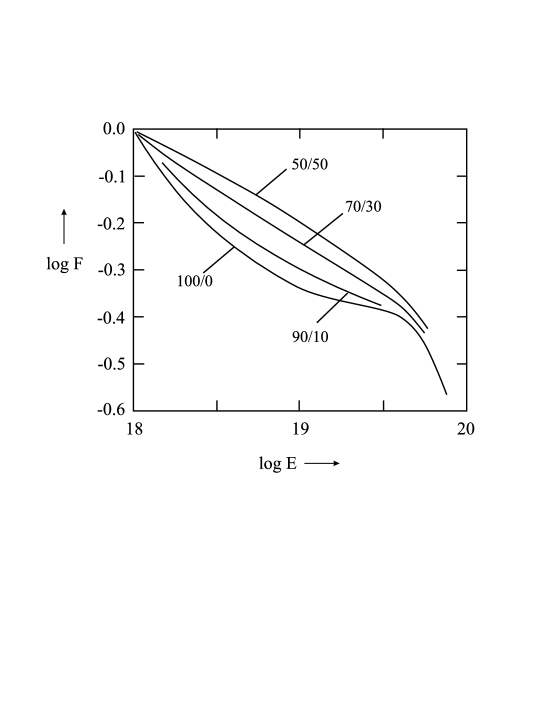
V.1 Sharpness for a mixed composition
Insofar as the energy-loss rates for protons – and nuclei (eg iron) are different, their sum will have a different shape to either. Figure 8 shows the equivalent to Figure 7. For the best estimate of the p/Fe mixture of 90/10, the sharpness is very small, and at too low an energy.
VI Conclusions
A variety of evidence leads us to believe that the ankle in the primary energy spectrum is due to the rapid transition from Galactic to Extragalactic particles and is not due to Extragalactic particles alone, which are required to predominate above logE = 18.0. In our model, at logE=19.0, 30%– 40% of the particles are still Galactic, although this fraction is falling rapidly with increasing energy. In ‘competing models’ this fraction is 10% for the Hi-Res case 2 , 2% in the ‘Hillas-model’ 4 and zero in the Berezinsky et al. model 3 .
Acknowledgements.
The authors are grateful to A.M.Hillas for useful comments,and for making available the details of his model.References
- (1) J. Szabelski et al., Astropart.Phys. 17, 125 (2002).
- (2) G. Thompson et al., Proc.Catania Cosmic Ray Conference (2004).
- (3) V.S. Berezinsky et al., Astropart. Phys. 21, 617 (2004).
- (4) A.M. Hillas, Proc. Leeds Cosmic Ray Conference (2004).
- (5) A.D. Erlykin and A.W. Wolfendale, J.Phys.G 23, 979 (1997).
- (6) A.D. Hillas (private communication)
- (7) G. Archibold et al., Proc. 28th ICRC, Tsukuba, 1, 405 (2003).
- (8) V.S. Berezinsky and S.I. Grigor’eva, Astron.Astrophys. 199, 1 (1988).
- (9) S. Yoshida and M. Teshima, Prog. Theor.Phys. 89, 833 (1993).
- (10) R.J. Protheroe and P. Johnson, Astropart.Phys. 4, 253 (1996).
- (11) I. Robson, Active Galactic Nuclei, John Wiley & Sons, Chichester (1996).
- (12) A.W. Strong et al., J.Phys.A 7, 1489; 1767 (1974).
- (13) S.S. Al-Dargazelli et al., J.Phys.G 22, 1825 (1996).
- (14) S. Yoshida and M. Teshima, Prog. Theor. Phys. 89, 833 (1993).
- (15) W.J. Frith et al., Mon. Not. Royal Astronomical Society 345, 1049 (2003).
- (16) T. Wibig and A.W. Wolfendale, J.Phys.G 25, 1099 (1999).
- (17) X. Chi et al., J.Phys. G. 20, 673 (1994).
- (18) M.T. Dova et al., Proc 28th ICRC, Tsukuba, 1, 377 (2003).
- (19) K. Shinosaki et al., Proc. 28th IRC, Tsukuba, 1, 401 (2003).


(c, d) The world average data after subtraction of the Galactic component. The line corresponds to a spectrum with slope . It is evident that a smoothly falling Galactic spectrum results in an EG spectrum that is a simple power law for energies below log E 19.4.
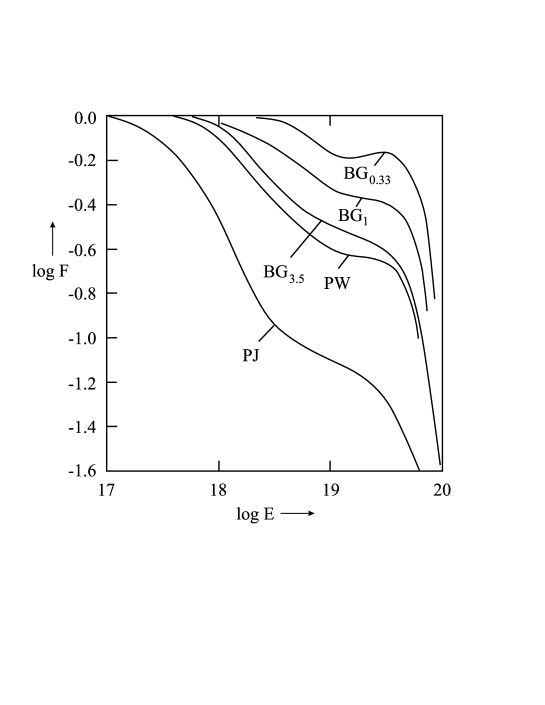
BG: Berezinsky and Grigor’eva [8] for no cosmological increase in injection spectrum with increasing red shift, but integrating out to various maximum -values (eg BG3.5 means integrating to )
PW: ‘present work’ from Figure 5.
PJ: Protheroe and Johnson [10]: this includes a cosmological increase in injection with increasing .
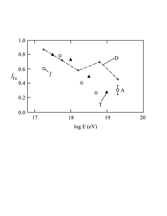
Origin of the estimates: : frequency of shower maximum values [16], T: ‘trajectories’ for Galactic particles [17], A: Akeno [19], D: Doveet al. [18].
There seems little doubt that there are heavy nuclei at log E = 19.
| array | sharpness | ||
|---|---|---|---|
| 1 | 2 | 3 | |
| Akeno∗ | 2.68 | 2.68 | 0.86 |
| AGASA | 0.99 | 1.03 | 0.85 |
| Fly’s Eye | 1.06 | 0.98 | 0.93 |
| Hi Res I+II | 0.58 | 0.98 | 0.90 |
| Haverah Park | 0.62 | 0.83 | 0.91 |
| Yakutsk 1+2 | 0.90 | 0.80 | 0.78 |
| Mean S | 0.83 | 0.92 | 0.870.02 |
| ————————– |
| The Akeno values are uncertain and have not been used in the analysis. |
| key: | |
| 1: | Fits to all the data points. |
| 2: | Fits excluding those within of the minimum. |
| 3: | As 2 but with one, universal index (EG exponent) for all experiments. |