Beam mismatch effects in Cosmic Microwave Background polarization measurements

Measurement of cosmic microwave background polarization is today a major goal of observational cosmology. The level of the signal to measure, however, makes it very sensitive to various systematic effects. In the case of Planck, which measures polarization by combining data from various detectors, the beam asymmetry can induce a conversion of temperature signals to polarization signals or a polarization mode mixing. In this paper, we investigate this effect using realistic simulated beams and propose a first-order method to correct the polarization power spectra for the induced systematic effect.

1 Introduction

After the success of COBE (Smoot et al, smoot (1992)) and WMAP (Bennett et al. Bennett (2003) , the Planck mission, to be launched by ESA in early 2007, is the third generation space mission dedicated to the measurement of the properties of the Cosmic Microwave Background (CMB). About 20 times more sensitive than WMAP, Planck will observe the full sky in the millimeter and sub-millimeter domain in nine frequency channels centered around frequencies ranging from 30 to 70 Ghz (for the Low Frequncy Instrument, or LFI) and from 100 to 850 GHz (for the High Frequency Instrument or HFI). Of these channels, the seven at lowest frequencies — from 30 to 350 GHz, are polarization sensitive.

Temperature anisotropies have been detected by many experiments now, the most recent of which detect a series of acoustic peaks in the CMB spatial power spectrum (de Bernardis et al, boom1 (2000), Hanany et al, maxima1 (2000), Benoît et al, archeops1 (2003), Hinshaw et al, wmapcl (2003)), confirm the Gaussianity of observable CMB fluctuations (Komatsu et al, wmapgauss (2003), though wavelet methods have detected presence of non-Gaussianity in WMAP data, Vielva et al, vielva (2004)), and demonstrate the spatial flatness of the Universe (Netterfield et al, Netterfield (2002), Lee et al, maxima2 (2001), Benoît et al, archeops2 (2003), Spergel et al, wmapcp (2003), Spergel et al, wmapcp3 (2006)). This provides compelling evidence that the primordial perturbations indeed have been generated during an inflationary period in the very early Universe. The next challenge now is the precise measurement of polarization anisotropies and, in particular, the detection of the pseudo-scalar part of the polarization field (the $B$ modes of CMB polarization) which are expected to carry the unambiguous signature of the energy scale of inflation and of the potential of the inflationary field. The Planck mission will be the first experiment able to constrain significantly these $B$ modes over the full sky and hence to measure them on very large scales.

The first detection of CMB polarization at one degree angular scale of resolution, at a level compatible with predictions of the standard cosmological scenario, has been announced by Kovac et al (Kovac (2002)) (see also Leitch et al Leitch (2004)). Since then, CBI and CAPMAP have also obtained significant detection of CMB E–mode polarization (Readhead et al. Readhead (2004) and Barkats et al. Barkats (2005)). More recently, the Boomerang (Piacentini et al Piacentini (2005), Montroy et al Montroy (2005)) and WMAP (Kogut et al. Kogut (2003), Page et al. Page (2006)) teams have obtained a measurement of the temperature-polarization correlation and E–mode spectrum compatible with cosmological model. No significant constraint on B–mode at degree angular scales exist today.

While the measurement of the temperature and polarization auto and cross power spectra of the CMB carries a wealth of information about cosmological parameters and about scenarios for the generation of the seeds for structure formation, some near–degeneracies exist which require extremely precise measurements. In particular, a very precise control of systematic errors is required to constrain parameters which impact these anisotropies and polarization fields at a very low level.

Many sources of systematic errors are potentially a problem for polarization measurements. In particular, the shape of the beams of the instrument need to be known with extreme precision. In addition, when the measurements of several detectors are combined to obtain polarization signals, it is required that the responses of these detectors be matched precisely in terms of cross–calibration, beam shape, spectral response, etc.

Measurements of Planck telescope beams in the actual operation conditions are not to be made on ground. Also, there are no polarized astrophysical sources for the in-flight beam calibration. Therefore, one should rely on numerical simulations of the beams and self-correcting algorithms of data processing that should allow efficient elimination of systematic errors. In polarization measurements, a significant systematic error would arise due to elliptical shapes of telescope beams which appear, mainly, due to ellipsoidal shape of telescope mirrors introducing astigmatic aberrations and other beam imperfections even with the otherwise ideal mirror surfaces.

In this paper, we investigate the impact of beam imperfections on the measurement of polarization power spectra. We then discuss a method for first-order correction of the effect of these imperfections. To illustrate this method, we apply it to the case of Planck HFI polarization measurement.

The remainder of this paper is organized as follows. In section 2, we discuss the issue of beam shape mismatch for the detection of CMB polarization. Section 3 is dedicated to the computation of simulated readouts using the realistic beams described in Section 2 and the reconstruction of polarized power spectra. In Section 4, we present a method to correct for the systematic bias in the $B$ mode power spectrum induced by the asymmetry of the beams. Finally, Section 5 draws the conclusions.

2 The beam–mismatch problem in polarization measurements

The HFI polarimeters employ Polarization Sensitive Bolometers (PSB) cooled down to the temperature of 100 mK by a space ³He –⁴He dilution fridge. These devices, also used on Boomerang (though at 300 mK), are presently the most sensitive operational detectors for CMB polarization measurements (Jones et al., psb (2003), Montroy et al., b2k (2003)). Each PSB measures the power of the CMB field component along one linear direction specified by the PSB orientation (Turner et al, PSB (2001)).

Ideally, the PSBs are combined in pairs, each pair placed at the rear side of respective HFI horn, with the two PSB of the pair, $a$ and $b$, being oriented at $90^{\circ}$ of relative angle and receiving the radiation from the same point on the sky. The ideal polarimeters produce the measured signals (readouts):

$$s_{a}=\frac{1}{2}(I+Q\cos 2\alpha+U\sin 2\alpha)$$ (1)

$$s_{b}=\frac{1}{2}(I-Q\cos 2\alpha-U\sin 2\alpha)$$ (2)

where $I$, $Q$, $U$ are the Stokes parameters of incoming radiation (see e.g. (Born and Wolf, born (1997)) for the definition of Stokes parameters) and $\alpha$ is the angle between the orientation of the first ($a$) of two PSBs and the first ($x$) of two orthogonal axes of the frame chosen for the representation of Stokes parameters. The $V$ Stokes parameter does not enter Eqs. (1), (2) since the PSBs are designed to be, ideally, insensitive to $V$ and, besides, $V$ is extremely small for the CMB radiation.

In practice, the detectors produce beam–integrated signals so that equation 1 is modified to (Kraus Kraus (1986))

$$s_{a}=\frac{1}{2}\int_{\rm beam}{\rm d}\Omega\int_{\rm band}{\rm d}\nu\,({\widetilde{I}_{a}}I+{\widetilde{Q}_{a}}Q+{\widetilde{U}_{a}}U+{\widetilde{V}_{a}}V)$$ (3)

and similarly for $s_{b}$ where the PSB responses ${\widetilde{I}_{a}}(\@vec{x},\nu)$ etc are the telescope beam patterns of Stokes parameters computed in transmitting mode and normalized to unity at maximum, functions of both the radiation frequency $\nu$ and the observation point $\@vec{x}$ (the $V$ term is neglected in most of the following discussion). The responses of different polarimeters (a and b) should be adjusted as much as possible (both in frequency and in angular pattern on the sky) so that, ideally, one should have

$${\widetilde{I}_{a}} = {\widetilde{I}_{b}}$$ (4)

$${\widetilde{Q}_{a}} = \ \ {\widetilde{I}_{a}}\cos 2\alpha,\quad{\widetilde{U}_{a}}=\ \ {\widetilde{I}_{a}}\sin 2\alpha,$$ (5)

$${\widetilde{Q}_{b}} = -{\widetilde{I}_{b}}\cos 2\alpha,\quad{\widetilde{U}_{b}}=-{\widetilde{I}_{b}}\sin 2\alpha$$ (6)

$${\widetilde{V}_{a}} = {\widetilde{V}_{b}}=0$$ (7)

where $\alpha$, similarly to the definition above, is the angle of nominal orientation of polarimeter $a$ on the sky with respect to the reference axis chosen for the definition of $Q$ and $U$. In this case, with $\widetilde{I}_{a}=\widetilde{I}_{b}$, Eq. (3) is reduced to the form similar to Eqs. (1) and (2).

For simplicity, we approximate the PSB response as averaged over the frequency band of the particular channel, thus introducing the band–averaged beam patterns defined as

$$\widetilde{I}(\@vec{x})=\int_{\rm band}{\rm d}\nu\,{\widetilde{I}}(\@vec{x},\nu)$$ (8)

and similarly for $\widetilde{Q}$ and $\widetilde{U}$ (for radiation independent on $\nu$ on the beam width scale, this generates an exact readout).

Ideally, the beam patterns on the sky ${\widetilde{I}}(\@vec{x})$ should be as close as possible to a perfect Gaussian. Unfortunately, design and construction imperfections, telescope aberrations, and optical misalignment all generate small differences in the beam patterns, the impact of which must be investigated accurately, especially for very sensitive CMB polarization measurements.

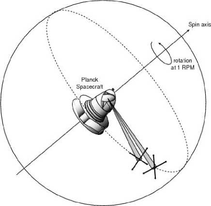
(a) (b)

Figure 1: (a) The scanning of the polarized detectors provides the measurements of intensity of the CMB field components along four directions at each point on the scan path. (b) Definition of axis specifying the Stokes parameters reference frame as seen from the sky. The detector pair on the left (e.g. 143-4) measures the $Q$ Stokes parameter, while the pair on the right (e.g. 143-2) measures $U$ when $Q$ and $U$ are defined with respect to the $(x_{\alpha},y_{\alpha})$ frame (see Appendix A for further detail on reference axis).

Measuring polarization, i.e. measuring the $I$, $Q$ and $U$ Stokes parameters, indeed involves combining several such measurements with different angles $\alpha$ to separate the $I$, $Q$ and $U$ contributions. The Planck HFI detector set–up is such that the beams of two horns with complementary pairs of PSB oriented at 45^∘ one pair with respect to the other follow each other on circular scan paths on the sky as shown in Figs. 1 and 2 (see Appendix A for further detail and notations). Then, in a system where reference axes for defining $Q$ and $U$ are along the scan path ($x$) and orthogonal to it ($y$), the four readouts $s_{\alpha}$ of this set of PSB ($\alpha=0^{\circ},45^{\circ},90^{\circ},135^{\circ}$) allow the direct measurement of $I$, $Q$ and $U$ as

$$I = s_{0^{\circ}}+s_{90^{\circ}}=s_{45^{\circ}}+s_{135^{\circ}}$$

$$Q = s_{0^{\circ}}-s_{90^{\circ}}$$ (9)

$$U = s_{45^{\circ}}-s_{135^{\circ}}.$$

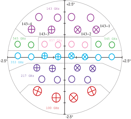
Figure 2: Planck focal plane unit (FPU) with polarization sensitive bolometers as seen from the sky. Complementary pairs of PSB detectors are arranged in two horns following each other while scanning the sky so that four detectors are in an optimized configuration for polarization measurement.

In practice, when the responses ${\widetilde{I}_{0^{\circ}}}$ and ${\widetilde{I}_{90^{\circ}}}$ are not perfectly equal, there is a small residual of $I$ in the estimate $\widehat{Q}$ of $Q$:

$${\widehat{Q}}=Q+\frac{1}{2}\int_{\rm beam}{\rm d}\Omega({\widetilde{I}_{0^{\circ}}}-{\widetilde{I}_{90^{\circ}}})I.$$ (10)

Similarly, there may be a small leakage of each Stokes component into the others. These errors are a source of trouble for measuring $B$ mode especially, as they result in the leakages of $I$ into $E$ and $B$ (possibly significant) and of $E$ into $B$ because $I\gg E\gg B$ on most scales.

This source of systematic effects for polarization measurements is not specific to Planck. Any instrument measuring polarization in a similar way, where signals proportional to $I$ need to be eliminated from the measurements in order to obtain polarization data, may suffer from this.

The quantitative investigation of the impact of such effects requires a realistic estimate of mismatch between the companion beams, the simulation of signal data using these beams, the reconstruction of maps and of power spectra using these simulated data, and the investigation of the correction of the effect by data processing methods.

The computation of the Planck HFI beams is discussed in Appendix A and in (Yurchenko et al., 2004b ). Here, we will describe their main characteristics relevant for the following sections. Because of telescope aberrations, the shape of the intensity beams is essentially Gaussian elliptic (down to nearly -30 dB) with the major axis around 10% longer than the minor axis (see Fig. 3). Thanks to the use of PSB, the intensity beams of an orthogonal pair of detectors within one horn are very close to each other: the difference is at most 0.6%. On the other hand, the difference between beams of detectors in two different horns can be up to 7%: this difference is mainly due to the different orientation of the beam ellipses. As emphasized in Appendix A, relaxing the assumptions of perfect conductors and perfect alignment is not expected to strongly modify the general shape of the beams. In the next sections, we will refer to these computer-simulated beams as “realistic beams”.

(a) (b)

Figure 3: Broad–band power patterns ($\widetilde{I}$ responses) of the telescope beams to be superimposed on the sky for polarization measurements, (a) HFI-143-2a and (b) HFI-143-4a, in SC spherical frame on the sky, with the spin axis of telescope as a pole (isolevels are shown from the maximum down to $-60\,$dB with a step of $-3\,$dB).

3 Effect of beams on polarization power spectra

The main goal of this section is to study the systematic effect induced on the power spectra estimation by realistic beams described in the previous section, knowing that this effect will depend also on the scanning strategy. As the Planck mission will scan the sky along large opening angle circles, resulting in large parts of the sky where the scans are mostly parallel, we have focused the study to the observation of a $15^{\circ}\times 15^{\circ}$ region of the sky scanned only along parallel directions. This restriction does not spoil the interest of the study as the small scale distortion of the beams are expected to affect mainly the small angular scales of the power spectra. In addition, other experiments scanning only a fraction of the sky are affected by the similar systematic effects. This restriction also offers a practical advantage: the computation of the effects of tiny beam mismatches on sub-beam scales requires a map resolution better than the beam size. For the Planck HFI 143 GHz channel, the resolution of about 7 arcminutes justifies models at sub-arcminute scales. We have thus chosen to work on maps of $2048\times 2048$ pixels of about 30 arcseconds each.

The following paragraphs describe the generation of CMB polarization maps from power spectra, and the simulation of instrument signals.

3.1 Generation of CMB polarization maps

Simulated square maps of CMB intensity and polarization are generated using the approximate relation between the power spectra in flat ($C(k)$) and spherical ($C_{l}$) coordinates: $k^{2}C(k)\simeq\left.l(l+1)C_{l}\right|_{l=k}$ (see, for example, White et al White99 (1999)). The three maps of $T$, $E$ and $B$ are then computed from three independent realizations of Gaussian white noise $D^{1}(\mathbf{k})$, $D^{2}(\mathbf{k})$ and $D^{3}(\mathbf{k})$ as:

$$a^{T,B}(\mathbf{k})=D^{1,3}(\mathbf{k})\sqrt{C_{l}^{T,B}}$$

and

$$a^{E}(\mathbf{k})=D^{1}(\mathbf{k})\frac{C_{l}^{TE}}{\sqrt{C_{l}^{T}}}+D^{2}(\mathbf{k})\left(C_{l}^{E}-\frac{\left(C_{l}^{TE}\right)^{2}}{C_{l}^{T}}\right)^{1/2}$$

so that the correlation between the $T$ and $E$ maps is taken into account. $C_{l}$’s are the usual spectra describing the CMB temperature and polarization. For our simulations, we used the cosmological parameters from the WMAP best fit model, except that we imposed a tensor to scalar ratio of 0.1. The simulated maps include the Gaussian part of the gravitational lensing effect of the $E$ mode.

3.2 Simulation of instrument readouts

The readouts must be computed from the $I$, $Q$ and $U$ Stokes parameters. We thus need to convert the $E$ and $B$ maps to $Q$ and $U$ using relations (38) in Zaldarriaga & Seljak Zaldarriaga97 (1997):

$$a^{Q}(\mathbf{k})=a^{E}(\mathbf{k})\cos 2\phi_{\mathbf{k}}-a^{B}(\mathbf{k})\sin 2\phi_{\mathbf{k}}$$ (11)

$$a^{U}(\mathbf{k})=a^{E}(\mathbf{k})\sin 2\phi_{\mathbf{k}}+a^{B}(\mathbf{k})\cos 2\phi_{\mathbf{k}}$$ (12)

where $k_{x}+ik_{y}=k\mbox{e}^{i\phi_{\mathbf{k}}}$. The readout from one detector is then obtained by convolving its $\widetilde{I}$, $\widetilde{Q}$ and $\widetilde{U}$ beams with the $I$, $Q$ and $U$ maps from the sky and summing as in Eq. (3). In the case of the parallel scanning strategy we used, the convolution can be easily done, once for all directions of observation, by multiplication in Fourier space. Thus, we obtain four maps of readout signals, one for each polarization channel, $s_{0^{\circ}}$, $s_{90^{\circ}}$, $s_{45^{\circ}}$ and $s_{135^{\circ}}$, with polarization angles $\alpha=0^{\circ}$, $90^{\circ}$, $45^{\circ}$ and $135^{\circ}$ with respect to the $x$-axis of the map. With account of established focal plane unit (FPU) notation of channels (see Appendix A), they correspond, e.g., to the PSB channels 4b, 4a, 2b, and 2a, respectively, of two horns HFI-143-4 and HFI-143-2 where $x$-axis is the $\varphi_{SC}$-axis of spacecraft (SC, see Appendix A) frame viewed from the sky (Fig. 1b).

Since the goal of this work is to study only the systematic bias induced on polarization power spectra, we do not add any white or low-frequency noise to the signal, neither any other systematic effects (Kaplan & Delabrouille Kaplan (2002)). These other systematic effects will be studied in detail in a forthcoming paper. In particular, we assume here that the time constant of bolometers, which induce an elongation of the beams in the scanning direction, has been corrected for.

3.3 Reconstruction of the power spectra

The parallel scanning strategy allows us to reconstruct the $I$, $Q$ and $U$ maps from the readout maps using Eqs. (9). The reconstructed $E$ and $B$ maps can be obtained from $Q$ and $U$ using the reciprocal transformation of the equations (11) and (12). The power spectra are then estimated directly from the Fourier transform of the reconstructed $\widehat{I}$, $\widehat{E}$ and $\widehat{B}$ maps, by averaging the $\widehat{a}^{X}(\mathbf{k})\widehat{a}^{Y*}(\mathbf{k})$ in bins of width $\Delta k=\Delta l=20$ (with $X,Y\in\{I,E,B\}$). The recovered power spectra are then corrected for the smoothing effect due to the beams, which can be approximated in Fourier space by a factor $\exp[-l(l+1)\sigma^{2}]$. However, because of the pixelization of the maps, this approximation is not good enough. Instead, we have corrected the power spectra using the power spectrum of the intensity beam, $B(k)=\left\langle|\widehat{a}^{I}(\mathbf{k})|^{2}\right\rangle$, where $\widehat{a}^{I}(\mathbf{k})$ is the average of the intensity beams of the four detectors. This is exact if the beams are axially symmetric and identical, and otherwise provides a way to symmetrize the beams in Fourier space. We have used this correction in all the power spectra shown hereafter.

The $B$ mode power spectrum reconstructed by using an ideal circular Gaussian beam in both the readout and reconstruction computations (assuming Eqs. (5) and (6)) is shown on Fig. 4a. The points shown are the average of 450 simulations and the error bars represent the dispersion. The relative error is shown in Fig. 4b, demonstrating that the statistical error on the power spectrum reconstruction averaged over 450 simulations is less than 2%. Finally, Fig. 5 presents the histogram of the bias divided by the dispersion, which is well fitted by a Gaussian with unit dispersion as expected for the ideal case. Identical results are obtained with other power spectra ($T$, $E$ and $T$-$E$ correlation).

We can now use this tool to estimate the bias induced on the power spectra reconstruction by the realistic beam shapes described in section 2.

3.4 Effects of beams on polarization power spectra

We apply our algorithm (both the readout simulation and $C_{l}$ reconstruction) using the realistic beam patterns $\tilde{I}$, $\tilde{Q}$ and $\tilde{U}$ presented in section 2. The output power spectra shown in Fig. 6 and 7 are averaged over 450 simulations. The temperature power spectrum is perfectly recovered, while we can distinguish a small but systematic excess in the $E$ power spectrum at $l>2000$ and a systematic loss in the $T$-$E$ correlation for $l>1000$. The $B$ mode is strongly affected after the peak of the lensing signal at $l\sim 900$, with a bias of up to 50% of the signal at $l\sim 1500$, and about 10% around the lensing signal peak at $l\sim 1000$.

The spurious $B$ mode may come from leakage of either the temperature or the $E$ mode. In order to separate the two possible origins, we have done the same simulation using the realistic beams $\tilde{I}$, $\tilde{Q}$ and $\tilde{U}$ when computing both the readouts and $C_{l}$ reconstruction but with no input $E$ mode (and no $T-E$ correlation). The results for $T$-$E$, $E$ and $B$ power spectra are shown on Fig. 9 (the temperature power spectrum is not modified). We observe that the spurious $B$ mode is about three times smaller in this case, indicating that about 2/3 of the spurious $B$ seen with realistic input $E$ mode came from $E$ leakage. On the other hand, the level of the $E$ mode is much higher than would be expected if it came from a mixing from $B$ modes into $E$ modes.

In order to check this, we made a simulation with elliptic Gaussian beams identical for detectors within the same horn, but with different ellipse directions for different horns. We have assumed Eqs (5) and 6 to represent the ideal polarization sensitivity of the channels, so that there is no total intensity leakage into polarization signal due to beam difference, and, again, used no input $E$ mode. In this situation, the recovered $E$ mode is a small fraction of the input $B$ mode signal, i.e. much smaller than the recovered $E$ mode in the previous test. This means that the $E$ mode recovered in the previous test (using realistic beams) was not due to a leakage from $B$ modes to $E$ modes, but rather from a leakage from $T$ to $E$. We conclude that, both the $E$ mode and the spurious $B$ mode found with realistic simulated beams when there is no $E$ mode in the readout simulation, come from a temperature leakage due to the differences in the beam patterns between detectors within the same horn, which is up to 0.9% (Fig. 13a).

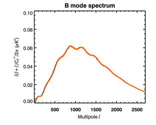
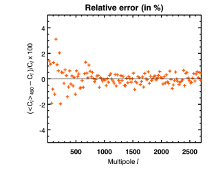
(a) (b)

Figure 4: (a) Input and recovered $B$ mode power spectrum with an ideal instrument, i.e. when four identical and axially symmetric Gaussian beams are used for both the readout generation and the $C_{l}$ reconstruction. The small peak at $l\sim 100$ is produced by the gravitational waves (the tensor to scalar ratio is $r=0.1$), while the main pattern peaking at $l\sim 1000$ is due to the lensing effect. The error bars are smaller than the thickness of the black solid line showing the input model. (b) The relative error between the recovered and the initial power spectrum; the recovered power spectrum is the average of 450 simultations: the statistical error is less than 2%, thus allowing the detection, in non ideal cases, of biases higher than 2%. Identical figures are obtained for $T$, $E$ and $T-E$ correlation power spectra.

Figure 5: Histogram of the biases divided by the statistical dispersion for all multipole bins shown on figure 4. As expected, the histogram is well fitted by a Gaussian of unit variance, showing that the dispersion on 450 simulations gives a good estimate of the errors.

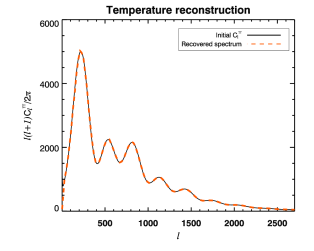
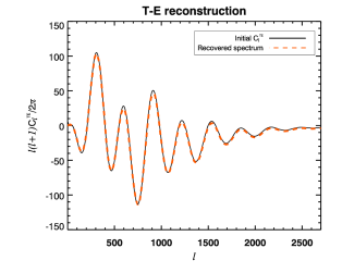
(a) (b)

Figure 6: Input and recovered power spectra of (a) temperature and (b) $T$-$E$ correlation signals, using the simulated beams of Sec. 2 for the readout simulation and the $C_{l}$ reconstruction. The recovered power spectra are corrected for an average symmetric beam effect by multiplying them by the power spectrum of the average beam map.

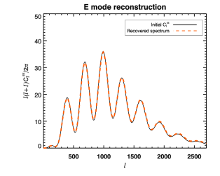
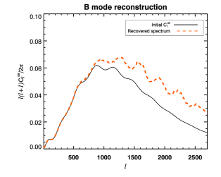
(a) (b)

Figure 7: Input and recovered power spectra of (a) $E$ mode and (b) $B$ mode signals, using the simulated beams of Sec. 2 for the readout simulation and the $C_{l}$ reconstruction. The recovered power spectra are corrected for an average symmetric beam effect by multiplying them by the power spectrum of the average beam map.

Figure 8: Recovered $B$ mode power spectrum in a simulation with no initial $B$ mode. The theoretical $B$ mode power spectra due to primordial gravitational waves are also shown for different values of the tensor-to-scalar ratio : 0.1, $10^{-3}$, $10^{-5}$ and $10^{-6}$ from top to bottom.

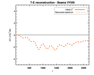
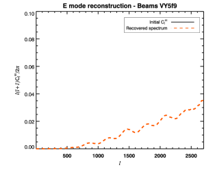
(a) (b) (c)

Figure 9: Spurious generation of $E$ and $B$ modes from temperature signals using simulated beams of Sec. 2 for the readout simulation and the $C_{l}$ reconstruction, but with no initial $E$ mode.

We thus see that two different effects produce the observed spurious $B$ mode. First, there is a mixing between the two polarization modes, essentially from $E$ to $B$ as $E\gg B$ on all scales, due to the beam mismatch between the two different horns. Second, there is a temperature leakage, this time due to the beam mismatch between the PSB within the same horn.

As seen on Fig. 7, the beam asymmetry affects mainly the high-$l$ part of the power spectra (typically $l>500$). However, it is not negligible at low $l$, where the gravitational waves lie. The Fig. 8 shows the recovered power spectra when there is no initial $B$ mode in the simulation compared to the expected $B$ mode signal from gravitational for various tensor-to-scalar ratios. The leakage from $T$ and $E$ mode to $B$ mode power spectrum becomes greater than the gravitational wave $B$ mode signal for $T/S\lesssim 10^{-5}$.

3.5 Link with previous work

Various studies have been done on the systematic effects on CMB polarization measurements, in particular the exhaustive work by Hu et al., Hu2002 (2002) (referred to as HHZ hereafter). This paper tries to estimate analytically the systematic effects on $B$ mode power spectrum, using a second order expansion and relating the terms of the expansion to beam defects such as, for example, pointing error, ellipticity, monopole leakage or calibration. The different systematic effects are assumed to be described by a statistically isotropic field, with a power spectrum of the form :

$$C_{l}\propto\exp(-l(l+1)\alpha^{2}),$$ (13)

so that the leakage from $T$ or $E$ to $B$ can be written as a convolution between $EE$ or $TT$ and systematic effect power spectra (Eqs. 30 and 34 in HHZ).

In our approach, the $I$, $Q$ and $U$ maps are given through the signals of four detectors (Eqs. 9). In the quasi-ideal case of all $Q$ and $U$ beams defined by Eqs 5 and 6, but with intensity beams different between the two horns, it can be shown that the error on the $B$ mode power spectrum is given by :

$$\delta C_{l}^{BB}=\frac{\left\langle\left|\Delta\widetilde{I}_{13}(\mathbf{l})\right|^{2}\cos^{2}(2\phi_{l})\sin^{2}(2\phi_{l})\right\rangle_{\phi_{l}}}{B_{l}}C_{l}^{EE}(\sigma)$$ (14)

where $\Delta\widetilde{I}_{13}=\widetilde{I}_{1}-\widetilde{I}_{3}$ is the beam difference, $B_{l}$ is the average beam power spectrum and $C_{l}^{EE}(\sigma)$ is the power spectrum of the $E$ map convolved with the average beam. This form is a particular case of the one given by HHZ, and describes completely the systematic effects on the $B$ mode power spectrum due to the beam mismatch between horns. Note however that there is no mixing between different $l$ of the power spectra. The major difference with HHZ estimate is in the shape of the beam difference power spectrum (first factor in Eq. 14) which can be fitted by $C_{l}^{\delta I}\propto l^{4}$ in the interval $l\in\{1,\ldots,3000\}$, very different from HHZ assumption, Eq. 13.

In the particular case we consider (beam mismatch) our approach gives more realistic results, as we use accurate simulations of the beams. Moreover, the power spectrum of the defect due to beam mismatch we compute from these beams is very different to HHZ assumption, leading to a different estimate of the size of the effect.

4 Correction of polarization spectra for systematic errors

We shall now propose a simple way to correct for the spurious $B$ mode deduced from the observations of the previous section. The idea is to assume that temperature and $E$ mode maps are recovered well enough to estimate the $T$ and $E$ to $B$ mode leakage, if we know the beam patterns. We will discuss three cases of $C_{l}$ correction, depending on the knowledge of the beams. In all three cases, the initial readouts are generated with the realistic $\tilde{I}$, $\tilde{Q}$ and $\tilde{U}$ beam patterns of Sec. 2.

4.1 Perfect knowledge of the intensity beam pattern

In order to have an idea of the ability of the method to remove the spurious $B$ mode, we have tested it in the case of a perfect knowledge of the intensity beam patterns. However, because of the lack of polarized point sources with known polarization characteristic, we assumed that only the intensity beam patterns $\widetilde{I}$ were perfectly measured while the $\tilde{Q}$ and $\tilde{U}$ needed for the $C_{l}$ correction are computed using relations (5) and (6) with the relevant $\tilde{I}$ in all the three cases considered.

The method is as follows. By a quick analysis of the data, we would find maps and their corresponding power spectra similar to the ones shown in Figs. 6 and 7. Since the $T$ and $E$ mode power spectra are recovered with a very good approximation, we may assume that the recovered maps are good as well. Starting with the temperature and the $E$ mode maps, assuming no initial $B$ mode and using a precise knowledge of the beams, we could then simulate the instrument signals. From the previous consideration, we expect to find, from these simulated signals, a spurious $B$ mode polarization coming both from a temperature leakage and a polarization mode mixing. The $B$ mode power spectrum of this simulated signal should be an estimate of the spurious $B$ mode.

The result for the $B$ mode correction, using exact $\tilde{I}_{a}$ and $\tilde{I}_{b}$ and assuming relations (5) and (6) for the leakage estimation, is shown on Fig. 10. The correction allows us to reduce the bias down to less than 1% of the lensing signal in the interval $2<l<1500$.

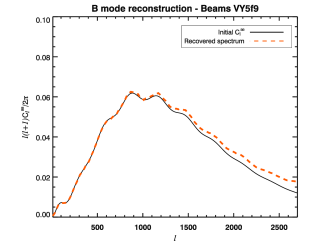
Figure 10: Recovered $B$ mode power spectrum before (red, dashed line) and after (green, dot-and-dashed line) correction. The power spectrum is corrected by subtracting the estimated leakage (blue dotted line) assuming knowledge of the exact beams (see text). Bottom: Difference between corrected and initial power spectra.

4.2 Assuming identical beams within the same horn

In a second case, we supposed that, in order to increase the signal to noise ratio, we need to use the signal from both detectors within one horn to measure the beam patterns. With this method, we would find as beam pattern the average of the beams of the two detectors within one horn, i.e. the average error on the beams is about 0.5% of the beam maximum.

The result obtained for the $B$ mode correction is presented on Fig. 11. This time, there is still some bias left in the corrected power spectrum, around 3% at $l\sim 1000$ and up to 13% for $l\sim 2100$.

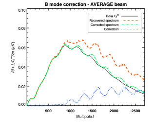
Figure 11: Recovered $B$ mode power spectrum before (red, dashed line) and after (green, dot-and-dashed line) correction. The power spectrum is corrected by subtracting the estimated leakage (blue dotted line) using beams averaged within one horn (0.5% error, see text). Bottom: Difference between corrected and initial power spectra.

4.3 Fitting the beams with elliptic Gaussians

If we have only few point sources or low signal-to-noise ratio on signal, we may want to parametrize the beam patterns with a function requiring a small number of parameters. As an example, we have fitted the four intensity beam patterns by elliptic Gaussian. The error of the fit is around 2% of the maximum of the beam.

The result is shown in Fig. 12, together with the difference between the corrected and initial $B$ mode power spectra. The result is very similar to that of Fig. 11 (using horn-averaged beams), though the remaining bias is slightly higher.

This simple method thus seems efficient to recover the right height of the lensing effect peak at $l\sim 1000$. Though it is applied here in the case of a simple scanning strategy (parallel scans), it should be applicable to any scan strategy, as soon as the bias estimation is done using the beams as precise as possible and the same scanning strategy as the real one.

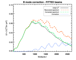
Figure 12: Recovered $B$ mode power spectrum before (red, dashed line) and after (green, dot-and-dashed line) correction. The power spectrum is corrected by subtracting the estimated leakage (blue dotted line) using elliptic Gaussian beams fitted on the exact beams (2% error, see text). Bottom: Difference between corrected and initial power spectra.

5 Conclusions

In this paper, we have shown the effect of asymmetric telescope beams on the bolometric measurements of polarization of incoming radiation by considering the case of the Planck satellite mission. We have used electromagnetic simulation of the optical system (including telescope and horns) to compute the main beam shapes of the different detectors of Planck. These beams are roughly Gaussian elliptical, with a major axis 10% larger than the minor axis and with essentially different orientations of the beam ellipses for the two horns to be combined to measure the full set of Stokes parameters, $I$, $Q$ and $U$.

By simulating the scan of a patch of the sky by Planck with these realistic, simulated beams, we have estimated the bias induced on the $E$ and $B$ mode polarization spectra due to their asymmetric shapes. We first remark that the $E$ mode power spectrum is very well recovered (once corrected for an effective symmetric beam), the bias being around 0.1% of the signal in the multipole range $300<l<2000$, where lies the most interesting part of the signal. On the other hand, the $B$ mode is affected by a bias around 10% at the peak of the lensing signal ($l\sim 1000$) and increasing for higher $l$, up to 100% of the signal at $l\sim 2500$. This bias has two origins. First, it is produced by the difference of beam patterns of two different horns combined to measure $Q$ and $U$. This difference induces mainly an error on the polarization angle, which turns to a mixing of $E$ and $B$ modes. Since, in general, $E\gg B$, we observe finally a leakage from $E$ to $B$. The second origin of the bias is the minor difference of beam patterns of two PSB channels with orthogonal polarizations within the same horn, which induces a temperature to polarization leakage.

Finally, we have proposed a way to correct the $B$ mode power spectrum from the above bias in a one-step correction which uses the measured $T$ and $E$ maps to compute the expected leakage into $B$ when they are observed with a model of the instrument’s beams. The efficiency of this correction depends on the precision of the beam knowledge: for example, using elliptical Gaussian fits of the actual beams allows us to reduce the bias from 10% to 3% at the lensing signal peak, $l\sim 1000$. In all cases, this first order correction has been shown to reduce significantly $B$ mode contamination. More refined treatments, currently being investigated, are expected to be yet more efficient if needed.

Appendix A Simulation of the Planck HFI telescope beams

It will not be possible to measure HFI beams on ground. The HFI bolometers indeed work only at 100 mK and are designed for the thermal load of a few Kelvin environment in space. Whereas the instrument can be put in a large vacuum tank cooled to 4 K, it is not possible to perform far field measurements of the full system, which would require placing a source hundreds of meters away from the instrument. Hence, responses can only be measured at subsystem level (e.g. bolometers + horns) and must be associated to a physical model of the telescope to predict the beam shape of the complete integrated optical system.

In this paper, for the investigation of beam mismatch effects, we use computer-simulated Planck HFI beams. We consider four HFI-143 beams comprising eight PSB channels used for the polarization measurements in the band centered at the frequency $\nu=143$ GHz. The polarization direction of each PSB is specified by the polarization angle $\psi$ on the sky and labeled by the relevant index of the channel ($\psi_{1a}$, $\psi_{1b}$ etc) as shown in Fig. 1(b).

In the design of the focal plane unit (FPU), the polarization angles $\psi_{i\alpha}$ notifying the channels are measured from the upward direction of local meridian of the spherical frame of spacecraft (SC) having the geometrical spin axis of telescope as a pole and counting the angles $\Psi$, as viewed from telescope, clockwise toward the direction of maximum polarization sensitivity of the channel. Similarly, we define the polarization angle $\psi$ at each observation point $\@vec{x}$ in the beam pattern. The direction of maximum polarization sensitivity is the major axis of polarization ellipse at point $\@vec{x}$; for the angles $\psi_{i\alpha}$ notifying the channels, $\@vec{x}$ is the beam axis defined as the point of maximum intensity $\widetilde{I}$ (at this point, the beam field is linearly polarized).

Following this definition, we consider eight PSB channels of the HFI-143 beams which are sensitive to the linearly polarized radiation with polarization angles on the sky $\psi_{1a}=\psi_{2a}=45^{\circ}$, $\psi_{1b}=\psi_{2b}=135^{\circ}$, $\psi_{3a}=\psi_{4a}=0^{\circ}$, and $\psi_{3b}=\psi_{4b}=90^{\circ}$. The four beams are arranged in two pairs (1 and 3, 2 and 4), with two beams of each pair scanning the sky along the same scan path as shown in Figs. 1 and 2. In each pair of beams, the angles $\psi_{i\alpha}$ correspond to a full set of four PSB detectors for polarization measurements with optimized polarimeter configuration (Couchot et al, Couchot (1999)).

The power patterns of two beams tracing the same scan path, HFI-143-2-a/b and HFI-143-4-a/b, are shown in Fig. 3 as projected on the sky in the spherical frame SC with coordinates $\varphi_{SC},\theta_{SC}$ ($\eta_{SC}=90^{\circ}-\theta_{SC}$) where the azimuthal angle $\varphi_{SC}$ is counted to the right from the optical axis of telescope as viewed from the sky and the polar angle $\theta_{SC}$ is measured from the upward direction of nominal spin axis (the optical axis of the telescope corresponds to $\varphi_{SC}=0^{\circ}$ and $\eta_{SC}=5^{\circ}$).

Notice that both the $a$,$b$ labels of channels and polarization angles $\psi$ are conventionally defined with respect to meridians (verticals) of the SC frame viewed from telescope, as accepted by the FPU design. In the meantime, because of the scanning strategy, the reference axes for the Stokes parameters on the CMB maps are usually parallels (horizontals) of the SC frame viewed from the sky to the telescope.

To reconcile these definitions, we continue to use the polarization angles $\psi$ and the established notations $a$,$b$ for the PSB channels. In the same time, for processing the readouts according to Eqs. (1)–(3), we define beam responses ${\widetilde{I}}$, ${\widetilde{Q}}$, ${\widetilde{U}}$, ${\widetilde{V}}$ in SC frame viewed from sky, with the first and the second reference axes being the azimuth $\varphi_{SC}$ and the elevation $\eta_{SC}$, respectively (they constitute the right-hand frame $xy$ for defining Stokes parameters on the sky as viewed from sky to telescope). With these definitions, the polarization angle in $xy$ frame is the angle $\alpha$ in Eqs. (1), (2) where $\alpha=\psi+90^{\circ}$.

The beams in Fig. 3 are computed with an extended version of the fast physical optics code (Yurchenko et al, FPO (2001)) developed specifically for the efficient simulations of the Planck HFI beams. The extended code allows us to propagate via the telescope the aperture field of the HFI horns mode–by–mode at various frequencies. The aperture field is generated by the PSB bolometers considered as polarized black–body radiators (in the transmitting mode) located at the rear side of the horns. In this way, we obtain the band–averaged far-field patterns of Stokes parameter responses $\widetilde{I}$, $\widetilde{Q}$, $\widetilde{U}$, $\widetilde{V}$ of the broad–band telescope beams as produced by the actual corrugated horns (Yurchenko et al, 2002a ) rather than by simplified model feeds.

Rigorous computations of beams require scattering matrix simulations of horns (Murphy et al, horns (2002)). In this approach, the effective modes of the electric field at the horn aperture, $E_{nm}$, are represented via the canonical TE, TM modes ${\cal E}_{nj}$ of a cylindrical waveguide as follows

$$E_{nm}(\rho,\varphi)=\sum_{j=1}^{2M}S_{nmj}{\cal E}_{nj}(\rho,\varphi)$$ (15)

where $S_{nmj}$ is the scattering matrix computed by Murphy et al (horns (2002)) for each horn at various frequencies, $n=0,1,...,N$ is the azimuthal index and $m,j=1,2,...,2M$ are the radial indices accounting for both the TE ($m,j=1,...,M$) and TM ($m,j=M+1,...,2M$) modes.

Recent simulations of the HFI-143 beams (Yurchenko et al, 2004a ) were performed with the scattering matrices of size $20\times 20$ ($M=10$, $N=1$) using nine sampling frequencies spanning the band $\nu=123-163\,$GHz. Although the power patterns of these beams only slightly differ from those computed earlier (Yurchenko et al, 2002a ) with matrices $10\times 10$ and five sampling frequencies ($\Delta P<0.1\;$dB at $P=-3\;$dB and $\Delta P<1.5\;$dB at $P=-30\;$dB), the effect on the difference between the beams of different polarization and on the fine polarization properties of beams is noticeable. This suggests that the latter parameters could be sensitive to other features of the model as well.

In this paper, the HFI-143 beams are computed with two essential updates compared to (Yurchenko et al, 2004a ): the horn design is slightly altered so that the horns are now slightly elongated compared to those used earlier, and the horn positions are now the final ones, being defined by the parameter $R_{C}=1.2$ mm that specifies the refocus of the horn aperture with respect to the geometrical focus of telescope for each beam.

The horn positions were optimized to achieve the best resolution (the minimum beam width) of the broadband beams (this also maximizes the gain) so that the value $R_{C}=1.2$ mm is close to the optimal horn positioning. We use updated scattering matrices of size $20\times 20$ for representing the horn field and nine sampling frequencies for spanning the frequency band $\nu=121-165$ GHz which is characteristic of the updated horns.

At this stage, we assume smooth telescope mirrors with ideal elliptical shape, perfect electrical conductivity of their reflective surfaces, and with ideal positioning of both the mirrors and horn antennas. The convergence accuracy of computations was better than $0.1\%$ relative to the maximum of the beam intensity pattern $\widetilde{I}(\varphi,\eta)$ (for comparison, the difference of the broadband power pattern and the pattern computed at the central frequency is about $1\%$).

To be perfectly representative of what the actual beams may be, one should take into account possible misalignments of the optics, tilts and deformations of the mirrors, etc. In principle, however, tolerances on the alignment of mirrors and positioning of horns are such that the modifications they induce on the beams are supposed to be small, and we neglect this last issue for the present work.

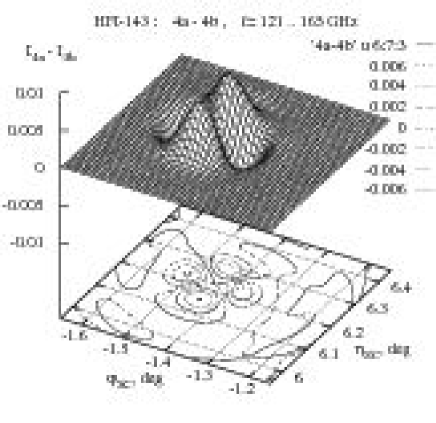
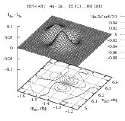
(a) (b)

Figure 13: Relative difference of power patterns (a) $\widetilde{I}_{4a}-\widetilde{I}_{4b}$ of two orthogonal channels of the same beam HFI-143-4 ($\psi=0^{\circ}$ and $\psi=90^{\circ}$, respectively) and (b) $\widetilde{I}_{4a}-\widetilde{I}_{2a}$ of the channels HFI-143-4a and HFI-143-2a ($\psi=0^{\circ}$ and $\psi=45^{\circ}$, respectively) when superimposed by spinning the telescope about the geometrical spin axis.

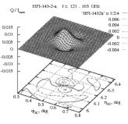
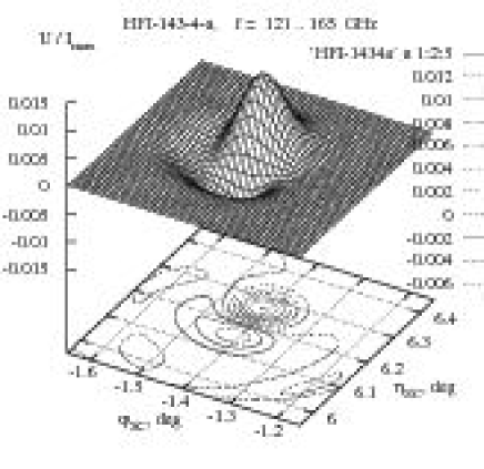
(a) (b)

Figure 14: The $\widetilde{Q}$ and $\widetilde{U}$ Stokes parameters responses: (a) $\widetilde{Q}$ of the beam HFI-143-2a and (b) $\widetilde{U}$ of the beam HFI-143-4a (ideally, both $\widetilde{Q}$ and $\widetilde{U}$ should be zero in the beams of these polarizations for the selected reference axes).

To minimize the beam mismatch between the channels of orthogonal polarizations, the PSB bolometers of each pair of channels, $a$ and $b$, are placed in the same cavity in the rear side of the respective horn and share the same optics — waveguides, filters, horns, telescope. Because of this design, the difference of power patterns of orthogonal polarizations of the same beam on the sky is really small (Fig. 13, a), with the peak value for all the broadband beams being about $\delta\widetilde{I}_{4a4b}={\rm max}(\widetilde{I}_{4a}-\widetilde{I}_{4b})/\widetilde{I}_{max}=0.6\%$ (at the central frequency $f=143$ GHz, the typical difference is $\delta\widetilde{I}_{4a4b}=0.9\%$).

A small difference of this kind arises for two reasons: (a) due to minor axial asymmetry of polarized modes that appears on the horn aperture when the PSB radiation (in the transmitting mode) propagates through the horn (the difference varies in sign and magnitude with frequency, though being well balanced over the band) and (b) due to some difference in the propagation of different polarizations along the same path via the telescope (all the differences are computed with the patterns normalized to the unit total power of the beams).

The mismatch of power patterns of different beams is about 10 times more significant (Fig. 13, b). It depends essentially on the location of horns in the focal plane of telescope. For the pair of beams HFI-143-2 and HFI-143-4, when superimposed on the sky by spinning the telescope until the coincidence of azimuths of beam axes, the peak difference of the relative power across the pattern varies from $7.0\%$ to $8.2\%$ depending on the polarizations being compared. Notice that the statistical difference of $5\%$ is already rather crucial for the reliable reconstruction of the CMB polarization map (Kaplan et al, Kaplan (2002)).

Fig. 14 shows the patterns of $\widetilde{Q}$ and $\widetilde{U}$ Stokes parameter responses of the HFI-143-2a and HFI-143-4a beams, respectively. The peak values of these parameters are $\widetilde{Q}_{2a}=0.6\%$ and $\widetilde{U}_{4a}=1.2\%$ (ideally, $\widetilde{Q}$ and $\widetilde{U}$ should be zero in these polarizations). For comparison, the peak values of $\widetilde{V}$ are $3.7\%$ and $4.2\%$, respectively. The positive and negative values of $\widetilde{Q}$ and $\widetilde{U}$ (as well as $\widetilde{V}$) are well balanced over the beam patterns and the average is very close to zero. It proves that the chosen directions of polarization of the horn aperture field as found by optimizing on-axis beam polarization directions (Yurchenko,2002b ) are pretty good, even though the beam patterns are not quite symmetrical due to aberrations.

The analysis of different contributions to non-zero values of $\widetilde{Q}_{2a}$, $\widetilde{U}_{4a}$ and $\widetilde{V}$ shows that $\widetilde{V}$ arises mainly because of the field propagation via the telescope ($\widetilde{V}_{\rm max}$ on the horn aperture is only $0.5\%$). On the contrary, both $\widetilde{Q}_{2a}=0.6\%$ and $\widetilde{U}_{4a}=1.2\%$ given above and the power differences between the orthogonal channels of the same beams, $\delta\widetilde{I}_{2a2b}=\delta\widetilde{I}_{4a4b}=0.6\%$, are essentially due to the horn effects ($\widetilde{U}=0.4\%$ and $\delta\widetilde{I}_{ab}=0.8\%$ on the horn aperture). The telescope contribution, though non-additive, is still important, as the propagation of the axially symmetric quasi-Gaussian source field shows (in this case, $\delta\widetilde{I}_{2a2b}=0.9\%$ and $\delta\widetilde{I}_{4a4b}=1.0\%$ in the beams on the sky, being zero in the source field).

Finally, in the cross-beam power differences $\delta\widetilde{I}_{2\alpha 4\beta}$, both the horn and the telescope effects are significant (e.g., $\delta\widetilde{I}_{2\alpha 4\beta}$ depends, to some extent, on polarizations being compared), although the telescope effect dominates (for the quasi-Gaussian source field, $\delta\widetilde{I}_{2\alpha 4\beta}$ varies from $5.7\%$ to $6.7\%$ in a way consistent with the variations in the beams from the actual corrugated horns of respective polarizations).

References

- (1) Barkats, D. et al 2005, ApJ 619 L127-L130
- (2) Bennett, C. L. et al. 2003, ApJ Supp. 148, 1
- (3) Benoît, A., Ade, P., Amblard, A. et al. 2003, A&A Letter, 399, L19-L23
- (4) Benoît, A., Ade, P., Amblard, A. et al 2003, A&A Letter, 399, L25-L30
- (5) de Bernardis, P., Ade, P. A. R., Bock, J. J. et al. 2000, Nature, 404, 95
- (6) Born, M. and Wolf, E., 1997, Principles of Optics
- (7) Couchot, F., Delabrouille, J., Kaplan, J., & Revenu, B. 1999,A&A, 135, 579
- (8) Hanany, S., Ade, P., Balbi, A., et al. 2000, ApJ, 545, L5
- (9) Hinshaw, G., Spergel, D. N., Verde, L. et al. 2003, ApJS, 148, 135
- (10) Jones, W. C., Bhatia, R., Bock, J. & Lange, A. E. 2003, Proc. SPIE, 4855, 227
- (11) Kaplan, J. & Delabrouille, J. 2002, in Astrophysical Polarized Backgrounds, AIP Conf. Proc., 609, 209
- (12) Komatsu, E., Kogut, A., Nolta, M. et al. 2003, ApJS, 148, 119
- (13) Kogut, A. et al. 2003, ApJS, 148, 161
- (14) Kovac, J., Leitch, E. M., Pryke, C., Carlstrom, J. E., Halverson, N. W. & Holzapfel, W. L. 2002, Nature, 420 (6917), 772
- (15) Hu, W, Hedman, M. M. and Zaldarriaga, M., 2003, Phys. Rev. D, bf 67, 4, 043004
- (16) Kraus, J. D., 1986, Radioastronomy
- (17) Lee, A. T., Ade, P., Balbi, A., et al. 2001, ApJ, 561, L1
- (18) Leitch, E. M. et al. 2004, submitted to ApJ, astro-ph/0409357
- (19) Miller, A. D., Caldwell, R., Devlin, M. J., et al. 1999, ApJ, 524, L15
- (20) Montroy, T., Ade, P. A. R., Balbi, A. et al., 2003, New Astronomy Reviews, 47, 11-12, 1057
- (21) Montroy, T. E. et al., 2005, submitted, astro-ph/0507514
- (22) Murphy, J. A., Gleeson, E., Maffei, B. & Wylde, R. J. 2002, in 25th ESA Antenna Workshop on Satellite Antenna Technology, ed. K. van ’t Klooster & L. Fanchi (ESTEC, Noordwijk, The Netherlands) 649
- (23) Netterfield, C. B. et al. 2002, ApJ, 571, 604
- (24) Page, L., Hinshaw, G., Komatsu, E. et al. 2006, submitted, astro-ph/0603450
- (25) Piacentini, F. et al. 2005, submitted, astro-ph/0507494
- (26) Readhead, A. C. S., et al. 2004, Science, 306, 836-844
- (27) Smoot, G. F., Bennett, C. L., Kogut, A., et al. 1992, ApJ, 396, L1
- (28) Spergel, D. N., Verde, L., Peiris, H. V. et al 2003, ApJS, 148, 175
- (29) Spergel, D. N., Bean, R., Doré, O. et al 2006, submitted
- (30) Turner, A. D., Bock, J. J., Beeman, J. W., Glenn, J., Hargrave, P. C., Hristov, V. V., Nguyen, H. T., Rahman, F., Sethuraman, S. & Woodcraft, A. L. 2001, Appl. Opt., 40, 4921
- (31) Vielva, P., Martínez-González, E., Bareiro, R. B. et al 2004 ApJ, 609, 22
- (32) White, M., Carlstrom J. E., Dragovan, M. & Holzapfel, W. L., Astrophys.J., 1999, 514, 12
- (33) Yurchenko, V. B., Murphy, J. A. & Lamarre, J.-M. 2001, Int. J. Infrared & Millimeter Waves, 22, 173
- (34) Yurchenko, V. B., Murphy, J. A. & Lamarre, J.-M. 2002a, in 25th ESA Antenna Workshop on Satellite Antenna Technology, ed. K. van ’t Klooster & L. Fanchi (ESTEC, Noordwijk, The Netherlands) 281
- (35) Yurchenko, V. B. 2002b, in Experimental Cosmology at Millimetre Wavelengths, ed. M. De Petris, P.A. Moro & M. Gervasi, AIP Conf. Proc., 616, 234
- (36) Yurchenko, V. B., Murphy, J. A., Lamarre, J.-M. & Brossard, J. 2004a, Int. J. Infrared & Millimeter Waves, 25, 601
- (37) Yurchenko, V. B., Murphy, J. A. & Lamarre, J.-M. 2004b, Proc. SPIE Int. Soc. Opt. Eng. 5487, 542
- (38) Zaldarriaga, M. & Seljak, U 1997, Phys.Rev. D, 55, 1830-1840