Supernovae type Ia data favour coupled phantom energy

Abstract

We estimate the constraints that the recent high-redshift sample of supernovae type Ia put on a phenomenological interaction between dark energy and dark matter. The interaction can be interpreted as arising from the time variation of the mass of dark matter particles. We find that the coupling correlates with the equation of state: roughly speaking, a negative coupling (in our sign convention) implies phantom energy ($w_{\phi}<-1$) while a positive coupling implies “ordinary” dark energy. The constraints from the current supernovae Ia Hubble diagram favour a negative coupling and an equation of state $w_{\phi}<-1$. A zero or positive coupling is in fact unlikely at 99% c.l. (assuming constant equation of state); at the same time non-phantom values ($w_{\phi}>-1$) are unlikely at 95%. We show also that the usual bounds on the energy density weaken considerably when the coupling is introduced: values as large as $\Omega_{m0}=0.7$ become acceptable for as concerns SNIa. We find that the rate of change of the mass $\dot{m}/m$ of the dark matter particles is constrained to be $\delta_{0}$ in a Hubble time, with $-10<\delta_{0}<-1$ to 95% c.l.. We show that a large positive coupling might in principle avoid the future singularity known as “big rip” (occurring for $w_{\phi}<-1$) but the parameter region for this to occur is almost excluded by the data. We also forecast the constraints that can be obtained from future experiments, focusing on supernovae and baryon oscillations in the power spectra of deep redshift surveys. We show that the method of baryon oscillations holds the best potential to contrain the coupling.

I Introduction

One of the main open problems in Cosmology is to determine the properties of the unclustered component called dark energy that is required to explain CMB, supernovae Ia, cluster masses and other observational data.

Although most work on dark energy assumes it to be coupled to the other field only through gravity, there is by now a rich literature on possible interactions to standard fields and to dark matter. Even before the evidences in favor of dark energy, a coupling between a cosmic scalar field and ordinary matter has been studied by Wetterich wet88 ; wet90 while Damour, Gundlach and Gibbons dam investigated the possibility of a species-dependent coupling within the context of Brans-Dicke models. Generally speaking, any low-energy limit of higher-dimensional theories predicts the existence of scalar fields coupled to matter. More recently, several authors considered an explicit coupling between dark energy and matter: we denote this class of models as coupled dark energy. A partial list of works in this field is in refs. cq ; chim ; post2002 . Other authors considered a coupling to specific standard model fields: to the electromagnetic field carroll , to neutrinos horvat , to baryonic or leptonic current li : in these cases, there are strong constraints from local observations or from variation of fundamental constants.

In this paper we confine our attention to the interaction with dark matter, as in ref. cq . Such a coupling is of course observable only with astrophysical gf and cosmological aq experiments involving growth of perturbations or global geometric effects. Notwithstanding the large number of papers dealing with variants of coupled dark energy, the works dedicated to constraining the interaction via supernovae Type Ia (SNIa) are very limited. The main reason is that there is yet no compelling form of the interaction (just as there is no compelling form of the dark energy equation of state). To make a step towards constraining the energy exchange between the dark components, instead of considering a specific coupling motivated by (or inspired by) some fundamental theory, we adopt here a phenomenological point of view. That is, we assume a general relation between dark energy and dark matter and derive its theoretical and observational properties. Our simple relation includes several previous coupled and uncoupled dark energy models but extends the analysis to cases which have not been tested so far. The main aim of this paper is to derive bounds on the interaction strength by analysing the recent SNIa sample of Riess et al. riess2004 , which include several $z>1$ supernovae. This works extends previous investigations in ref. Dalal , which studied the same relation between dark matter and dark energy, and in ref. agp , which compared the recent SNIa data with a special class of coupled dark energy models motivated by superstrings and characterized by a constant ratio of densities.

II Modeling the interaction

Let us start with a model containing only dark matter and dark energy. The basic assumption of this paper is that the dark components interact through an energy exchange term. The conservation equations in FRW metric with scale factor $a$ can be written in all generality as

$$\begin{array}[]{ccc}\dot{\rho}_{m}+3H\rho_{m}&=&\delta H\rho_{m}\,,\\ \dot{\rho}_{{}_{\phi}}+3H\rho_{\phi}(1+\omega_{\phi})&=&-\delta H\rho_{m}\,,\end{array}$$ (1)

where the subscript $m$ stands for dark matter while the subscript $\phi$ stands for dark energy and where $\delta$ is a dimensionless coupling function. In principle the coupling $\delta$ might depend on all degrees of freedom of the two components. However, if $\delta$ is a function of the scale factor $a$ only then the first equation of (1) can be integrated out to give (we put the present value $a_{0}=1$)

$$\rho_{m}=\rho_{m0}a^{-3}e^{\int\delta d\alpha}\,,$$ (2)

where $\alpha=\log a$. This shows that the interaction causes $\rho_{m}$ to deviate from the standard scaling $a^{-3}$. That is, matter is not “conserved” or, equivalently, the mass $m$ of matter particles $\rho_{m}=m(a)n$, where $n$ is their number density, varies with time such that

$$\frac{m^{\prime}}{m}=\delta$$ (3)

where the prime denotes derivation with respect to $\alpha$. Therefore, $\delta$ can be interpreted as the rate of change of the particle mass per Hubble time.

While so far many paper have been devoted to find constraints on $w_{\phi}(a)$, aim of this paper is to derive constraints on $\delta(a)$ from SNIa. We need therefore a sensible parametrization of $\delta(a)$. Generally speaking, we are faced with two possibilities: either we write down a parametrization for $\delta(a)$ and then find from this the relation between $\rho_{m}$ and $\rho_{\phi}$, or first give the latter and derive a function $\delta(a)$. We find that this second choice is simpler and better connected to previous work and constraints.

The basic relation we start from is that the fluid densities scale according to the following relation Dalal

$$\rho_{\phi}/\rho_{m}=Aa^{\xi}$$ (4)

where $A,\xi$ are two constant parameters. Moreover, we approximate $w_{\phi}$ as a constant: it is clear however that a more complete analysis should allow for a time-dependent equation of state. The relation (4) has two useful properties: a) it includes all scaling solutions (defined as those with $\rho\sim a^{m}$) and b) the functions $\rho_{m}(a),\rho_{\phi}(a)$ can be calculated analytically. Since for uncoupled dark energy models with constant equation of state one has $\rho_{m}\sim a^{-3}$ and $\rho_{\phi}\sim a^{-3(1+w_{\phi})}$ it appears that the relation (4) reduces to this case for $\xi=-3w_{\phi}$. Conversely, if $\xi\not=-3w_{\phi}$ then the matter density deviates from the $a^{-3}$ law, as we have seen above.

The relation (4) has been first introduced and tested in ref. Dalal . The present paper extends their investigation in several respects. First, we include baryons. Ref. Dalal assumed a single matter component, but there are strong upper limits to an interaction of dark energy with baryons (i.e. upper limits to a non-conservation relation like Eq. (2) for baryons, see e.g. hagi ). We will assume therefore that baryons are uncoupled while the coupling to dark matter is left as a free parameter. This has important consequences for the general behavior of the model. Second, ref. Dalal confined the range of parameters to $0<\xi<3$ and $w_{\phi}>-1$, while we extend the range to a much larger domain, thereby including also the regime of “phantom” dark energy cald . Third, we use the new data of Riess et al. riess2004 : these include SN at $z>1$ and extend therefore by a considerable factor the leverage arm of the method. Fourth, we’ll discuss the implication of the results for as concerns the beginning of the acceleration. In riess2004 it was claimed that the new high-redshift SN constrain $z_{acc}<1$ (more exactly, $z_{acc}=0.46\pm 0.13$). In contrast with this, we show that $z_{acc}>1$ is not ruled out at more than 95% when the coupling is non-zero. A similar conclusion is obtained in ref. agp studying a string-motivated form of interaction and in bck adopting different parametrizations of the equation of state. Finally, we will produce forecasts for future experiments.

Before we include the baryons, let us derive some relations in the simplified case of two coupled components only. Assuming $\Omega_{tot}=\Omega_{\phi}+\Omega_{m}=1$ we obtain from (4):

$$\Omega_{\phi}+\frac{1}{A}a^{-\xi}\Omega_{\phi}=1\,,$$ (5)

so that the constant $A$ can be expressed in function of $\Omega_{\phi,0}$ (the subscript $0$ indicates the present epoch)

$$A=\frac{\Omega_{\phi,0}}{1-\Omega_{\phi,0}}\,.$$

If the dark matter is pressureless, $w_{m}=0$, the total energy density obeys the conservation equation

$$\frac{d\rho_{tot}}{da}+\frac{3}{a}(1+\omega_{\phi}\Omega_{\phi})\rho_{tot}=0\,.$$ (6)

Therefore, assuming a constant $w_{\phi}$, we obtain

$$\rho_{tot}=\rho_{0}a^{-3}[1-\Omega_{\phi,0}(1-a^{\xi})]^{-3\frac{\omega_{\phi}}{\xi}}\,,$$ (7)

and the Friedman equation

$$H^{2}=H_{0}^{2}a^{-3}[1-\Omega_{\phi,0}(1-a^{\xi})]^{-3\frac{\omega_{\phi}}{\xi}}\,.$$ (8)

It is worth remarking that this expression for $H^{2}$ cannot be reproduced by a simple model of varying $w$, as e.g. $w(z)=w_{0}+w_{1}z$. This means that the effect of the coupling is intrinsically different from the effect of a time-dependent equation of state.

The relation between the scaling behavior and the coupling $\delta$ is easily derived by imposing the relation (4)

$$\frac{d}{dt}(\frac{\rho_{\phi}}{\rho_{m}a^{\xi}})=0\,.$$ (9)

We find then

$$\delta=-\frac{(\xi+3\omega_{\phi})}{\rho_{\phi}+\rho_{m}}\rho_{\phi}\,.$$ (10)

Substituting (4) we obtain the evolution of the coupling as a function of $a$

$$\delta=\frac{\delta_{0}}{\Omega_{\phi,0}+(1-\Omega_{\phi,0})a^{-\xi}}\,,$$ (11)

where

$$\delta_{0}=-\Omega_{\phi,0}(\xi+3\omega_{\phi})\,.$$ (12)

III Adding the baryons

So far we assumed a single matter component. However, as already anticipated, if dark energy interacts with baryons then a new long-range force arises, on which there are strong experimental upper limits hagi ; dam . The baryonic component has therefore to be assumed extremely weakly coupled; for simplicity, we assume here that the baryons are totally uncoupled. In principle, of course, we should allow the possibility that also part of the dark matter itself is uncoupled, as in Ref. agp but for simplicity we restrict ourselves to the basic case in which all dark matter couples with the same strength. Here we derive the corresponding formulae when uncoupled baryons are added to the cosmic fluid. As it will appear clear, adding a small percentage of baryons at the present does not change qualitatively the fit to the supernovae; however, it changes dramatically the past and future asymptotic behavior of the cosmological model. In all the plots and numerical results we always assume $\Omega_{b,0}=0.05$. The parameter $A$ now becomes

$$A=\frac{\Omega_{\phi,0}}{1-\Omega_{b,0}-\Omega_{\phi,0}}\,,$$

from which

$$\delta=\frac{\delta_{0}(1-\Omega_{b,0})}{\Omega_{\phi,0}+(1-\Omega_{b,0}-\Omega_{\phi,0})a^{-\xi}}\,,$$ (13)

so that the present coupling is

$$\delta_{0}=-\frac{\Omega_{\phi,0}}{1-\Omega_{b,0}}(\xi+3\omega_{\phi})\,.$$ (14)

As it appears from Fig. 1, when $\xi>0$ the coupling varies from zero in the past to a constant value $\delta_{1}=-(\xi+3w_{\phi})$ in the future. As expected, the standard model of uncoupled perfect fluid dark energy is recovered when $\xi=-3w_{\phi}$. For $\xi<0$ the behavior is opposite. On the other hand, models with a constant $\delta$ (investigated in agp ) are obtained for $\xi=0$. In this case, $\rho_{\phi}\sim\rho_{m}$: such behavior has been called “tracking” dark energy when the regime is transient cald , and “stationary dark energy” cq ; bias when the regime is the final attractor. To emphasize the connection between $\xi$ and the coupling, we will use in most cases the present coupling $\delta_{0}=\delta(a=1)$ as free parameter instead of $\xi$. The parameters that characterize the model are therefore $(\Omega_{\phi,0},\omega_{\phi},\delta_{0})$. $\Lambda$CDM corresponds to $w_{\phi}=-1$ and $\delta_{0}=0$. The trend of the coupling $\delta$ can be expanded for low redshifts as

$$\delta\simeq\delta_{0}(1-z\frac{\xi\Omega_{m,0}}{1-\Omega_{b,0}})$$

The sign of $\xi$ is therefore also associated to the sign of the time derivative of the coupling.

The Friedman equation is now

$$H^{2}=H_{0}^{2}E(a)^{2}\,,$$ (15)

where

$$E^{2}=(1-\Omega_{b,0})a^{-3}[1-\frac{\Omega_{\phi,0}}{1-\Omega_{b,0}}(1-a^{\xi})]^{-3\frac{\omega_{\phi}}{\xi}}+\Omega_{b,0}a^{-3}\,,$$ (16)

which for $\xi=0$ becomes

$$H^{2}=H_{0}^{2}\{(1-\Omega_{b,0})a^{-\beta}+\Omega_{b,0}a^{-3}\}\,,$$ (17)

where $\beta=\frac{1-\Omega_{b,0}+3\omega_{\phi}\Omega_{\phi,0}}{1-\Omega_{b,0}}$.

It is interesting to derive the asymptotic limits of $\Omega_{b,m,\phi}$ (Figs. 2-4) Notice that, assuming $w_{\phi}<0$, the asymptotic future and past behaviour of the total density and of the density parameters of all the components depends only on the parameters $\xi$ . For $\xi>0$ we have the limits for $a\rightarrow 0$

$$\Omega_{b} \rightarrow \frac{\Omega_{b,0}}{(1-\Omega_{b,0})[1-\frac{\Omega_{\phi,0}}{1-\Omega_{b,0}}]^{-3\omega_{\phi}/\xi}+\Omega_{b,0}}\,,$$ (18)

$$\Omega_{m} \rightarrow 1-\Omega_{b}\,,$$ (19)

$$\Omega_{\phi} \rightarrow 0\,,$$ (20)

while for $\xi\leq 0$ we have $\Omega_{b}\to 1$ and $\Omega_{m},\Omega_{\phi}\to 0$, so that the baryons dominated the past evolution even if their present density is very low. The future asymptotics for $\xi>0$ is instead always dominated by dark energy,

$$\Omega_{b} \rightarrow 0\,,$$ (21)

$$\Omega_{m} \rightarrow 0\,,$$ (22)

$$\Omega_{\phi} \rightarrow 1\,,$$ (23)

For $\xi<0$ we have

$$\Omega_{b} \rightarrow \frac{\Omega_{b,0}}{(1-\Omega_{b,0})[1-\frac{\Omega_{\phi,0}}{1-\Omega_{b,0}}]^{-3\omega_{\phi}/\xi}+\Omega_{b,0}}\,,$$ (24)

$$\Omega_{m} \rightarrow 1-\Omega_{b}\,,$$ (25)

$$\Omega_{\phi} \rightarrow 0\,,$$ (26)

and finally for $\xi=0$,

$$\Omega_{b} \rightarrow 0\,,$$ (27)

$$\Omega_{m} \rightarrow \frac{\Omega_{\phi,0}}{1-\Omega_{b,0}}\,,$$ (28)

$$\Omega_{\phi} \rightarrow 1-\frac{\Omega_{\phi,0}}{1-\Omega_{b,0}}\,.$$ (29)

It could be assumed that the negative values of $\xi$ are to be excluded, since they imply absence of dark matter in the past. However, we are here studying the model only in a finite range of $z$ near the present epoch, and for this reason even negative $\xi$ cannot be excluded a priori. Moreover, baryons dominate in the past for $\xi<0$ and they could conceivably drive fluctuation growth. However, we will see that in fact values $\xi<0$ are not favoured by SN data.

There are other interesting features to remark in the general behavior of the density fractions. First, for $\delta_{0}\not=0$ the ratio $\Omega_{b}/\Omega_{m}$ varies in time. If $\xi>0,$ the ratio varies from a constant value in the past to infinity (if $\delta_{0}<0$) or zero (if $\delta_{0}>0$) in the future. If $\xi\leq 0$ the ratio decreases always (for $w_{\phi}<0$): this variation in the baryon-to-matter ratio due to the dark matter coupling could provide additional testing ground for the coupling (e.g. barfrac ).

Second, for $\xi<0$ the dark energy density vanishes both in the past and in the future, for all values of the equation of state: this means that the acceleration is only a temporary episode in the universe history, as shown in Fig. 4. The universe was dominated by the baryons in the past, by dark energy at the present and by a mix of baryons and dark matter in the future (for the parameters employed in Fig. 4 the final value of $\Omega_{b}$ is very low and cannot be distinguinguished from zero). For instance, assuming $w_{\phi}=-1,\Omega_{\phi}=0.7,\xi=-1$ it turns out that the acceleration ends in the future at $z=-0.85$. This is a particularly striking example of how the coupling might completely modify the past and future behavior of the cosmic evolution.

Another example comes from the existence of the future singularity known as “big rip”, i.e. an infinite growth of the total energy density in a finite time cald . From the Friedmann equation (16) we see that if $\xi>0$, for a large scale factor $H^{2}$ behaves as $a^{-3(1+w_{\phi})}$, as in the standard uncoupled model, so there is a big rip if $w_{\phi}<-1$. If, instead, $\xi<0$, then $H^{2}\sim a^{-3}$ . This means that a negative $\xi$ prevents the big rip for any value of $w_{\phi}$. From (14) we see that, assuming $\Omega_{b,0}\ll 1$, the big rip is prevented when

$$\delta_{0}>3|w_{\phi}|\Omega_{\phi,0}$$

However, we’ll find that this region of parameters space is rather disfavoured by SN data.

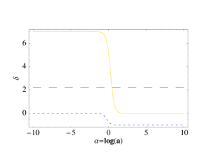
Figure 1: Behavior of $\delta(z)$ for $\Omega_{\phi}=0.7$ and $w_{\phi}=-1$. Full line: $\xi=-4$; dotted line: $\xi=4$; dashed line: $\xi=0$.

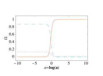
Figure 2: Behavior of $\Omega(a)$ for $\xi=4$ and $w_{\phi}=-1$, fixing $\Omega_{b,0}=0.05,$$\Omega_{m,0}=0.25$ and $\Omega_{\phi}=0.7$. Full line: dark energy; dotted line: baryons; dashed line: dark matter.

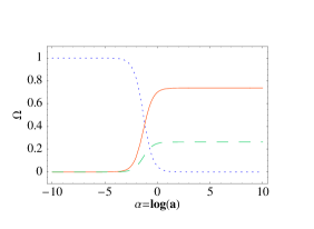
Figure 3: Behavior of $\Omega(a)$ for $\xi=0$ and $w_{\phi}=-1$ (the other parameters are as in the previous figure). Full line: dark energy; dotted line: baryons; dashed line: dark matter.

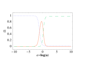
Figure 4: Behavior of $\Omega(a)$ for $\xi=-4$ and $w_{\phi}=-1$ (the other parameters are as in the previous figure). Full line: dark energy; dotted line: baryons; dashed line: dark matter.

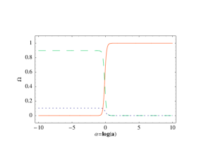
Figure 5: Behavior of $\Omega(a)$ for the best-fit values of $\xi$ and $w_{\phi}$ (the other parameters are as in the previous figure). Full line: dark energy; dotted line: baryons; dashed line: dark matter.

We are interested also in evaluating the epoch of acceleration. The acceleration begins when $\ddot{a}=0$ i.e. for ( $\xi\not=0$)

$$\frac{\ddot{a}}{a} = \frac{1}{2}H_{0}^{2}\{(\Omega_{b,0}-1)[1-\frac{\Omega_{\phi,0}}{1-\Omega_{b,0}}(1-a^{\xi})]^{-3\frac{\omega_{\phi}}{\xi}}-\Omega_{b,0}$$

$$-\frac{1}{2}\omega_{\phi}\Omega_{\phi,0}a^{\xi}[1-\frac{\Omega_{\phi,0}}{1-\Omega_{b,0}}(1-a^{\xi})]^{-3\frac{\omega_{\phi}}{\xi}-1}\}=0$$

which will be solved numerically later on. For $\xi=0$ the solution is

$$z_{acc}=[\frac{1-\Omega_{b,0}-3\omega_{\phi}\Omega_{\phi,0}}{\Omega_{b,0}}]^{\frac{1}{3-\beta}}-1\,.$$

Before starting with the data analysis, we need still another equation, the age of the universe. This is given by

$$T=H_{0}^{-1}\int_{0}^{1}\frac{da}{aE(a)}$$

where $E(a)$ is given in Eq. (16).

IV Comparing with SNIa

We used the recent compilation of SNe Ia data riess2004 (gold sample) to put constraints on the parameters $\Omega_{m,0},w_{\phi},\delta_{0}$ entering the expression for $H(a)$. In all subsequent plots we marginalize over a constant offset of the apparent magnitude, so that all results turn out to be independent of the present value of the Hubble parameter. In all the calculations we fix $\Omega_{b,0}=0.05$.

The overall best fit is $\Omega_{\phi,0}=0.62,w_{\phi}=-1.9,\delta_{0}=-1.5$ (see Fig. 5) with a $\chi^{2}$=173.7 (for 157 SN), to be compared to a $\chi^{2}=178$ for the flat $\Lambda$CDM. In Fig. 6 we present the main result of this paper: the contours at 68%, 95% and 99% of the likelihood function on the parameter space $\delta_{0},w_{\phi}$. The third parameter, $\Omega_{\phi,0}$, has been marginalized over with a Gaussian prior $\Omega_{\phi,0}=0.7\pm 0.1$. The $\Lambda$CDM model lies near 1$\sigma$ from the best fit. The line $\xi=0$ is tangent to the 3$\sigma$ contour: negative values of $\xi$ lie above this line and appear to be very unlikely with respect to positive values. It is impressive to observe how the vast majority of the likelihood lies below the uncoupled line $\delta_{0}$, which is almost tangential to the 1$\sigma$ contour, and leftward of $w_{\phi}=-1$. Taken at face value, this implies that the likelihood of a negative coupling (dark matter mass decreasing with time) contains 99% of the total likelihood, and that the likelihood of a phantom dark energy ($w_{\phi}<-1$) is 95% of the total likelihood. Our conclusion is therefore that the SNIa data are much better fitted by a negatively coupled phantom matter than by uncoupled, positively coupled or non-phantom stuff. It is interesting to note that it has been recently observed amprl that coupled phantom energy induces a repulsive interaction (regardless of the sign of the coupling).

In Figs. 7 and 8 we plot the 1-dimensional likelihood functions for $\delta_{0},w_{\phi}$, marginalizing over the other parameters. The main conclusion is that current supernovae data exclude a coupling $\delta_{0}>0$ at 99% c.l. if no priors are imposed on $w_{\phi}$. The lower bound is much weaker: a negative $\delta_{0}$ down to $\delta_{0}=-7$ is allowed to to 68%. At 95% level, the formal lower limit to $\delta_{0}$ is $-10$ but the convergence to zero is very slow and values very large and negative of $\delta_{0}$ cannot be excluded. In terms of the parameter $\xi$ we obtain $\xi>0$ at 95% c.l. while essentially no upper limit can be put with the same confidence. In terms of $m^{\prime}/m$, this implies that the dark matter mass can vary by a fraction $\delta_{0}$ in a Hubble time. Looking at Fig. 6 one sees that a zero or positive coupling is instead preferred if $w_{0}>-1$. Applying the prior $w_{\phi}>-1$ the limits on $\delta_{0}$ narrow and move to higher values: $-2.5<\delta_{0}<1.2$ (95%).

From Fig. 8 we see that $-3<w_{\phi}<-1.2$ at 68% and $-4.2<w_{\phi}<-1$ at 95% c.l.. In the same Fig. 8 we plot the likelihood for $w_{\phi}$ in the uncoupled case. As it can be seen, the coupled case extends considerably the allowed region of $w_{\phi}$, especially towards large and negative values: a negative coupling favors phantom equation of states. This complements the results of ref. agp in which it was found that a positive coupling (corresponding to a stationary behavior with $\xi=0$ and $w_{\phi}<0$) favours non-phantom matter. This is a clear-cut example of how the conclusions regarding the nature of dark energy depend crucially on its coupling to the rest of the world. It is intriguing that the correlation between $\delta_{0}$ and $w_{\phi}$ crosses approximatively the $\Lambda$CDM case $\delta_{0}=0,w_{\phi}=-1$: although not particularly favoured, $\Lambda$CDM remains a perfectly acceptable model also with respect to coupled dark energy.

We now impose on the 2D likelihood the contour levels of the acceleration (LABEL:eq:accb). Since a negative $\delta_{0}$ means a more recent surge of the dark energy it is to be expected that the likelihood favours a recent acceleration. It turns out that indeed the best fit corresponds to an acceleration epoch $z_{acc}\approx 0.3$; however, at the same time, an acceleration $z_{acc}>1$ lies near 2$\sigma$ and cannot be excluded with large confidence (Fig. 9), especially if one excludes phantom states of matter.

The age contours are compared to the likelihood in Fig. 10. Most of the likelihood lies within the acceptable range 11 and 14 Gyr (for $h=0.7$ and $\Omega_{\phi 0}=0.7$). The age constraints are therefore rather weak.

We can also marginalize on $\delta_{0}$ and plot the likelihood for $\Omega_{m0},w_{\phi}$ (see Fig. 11). In Fig. 12 we compare the likelihood for $\Omega_{m0}$ for the uncoupled case, $\delta_{0}=0$ and for the general case. Again the result is that the likelihood for $\Omega_{m0}$ widens considerably. Now practically any value from $\Omega_{m0}=0$ to $\Omega_{m0}=0.7$ is acceptable, with a broad peak around 0.25, while in the uncoupled case $\Omega_{m0}$ peaks rather tightly around 0.4 (remember that we are marginalizing over all values of $w_{\phi}$); if we restrict to $w_{\phi}>-1$ then we have roughly $0.1<\Omega_{m0}<0.3$ at 95%.

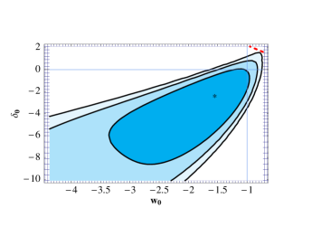
Figure 6: Likelihood contours at 68%, 95% and 99% c.l., inside to outside, marginalizing over $\Omega_{\phi}=0.7\pm 0.05$ (Gaussian prior). In this and the following two-dimensional plots the star marks the best fit; the horizontal line indicates the decoupled models, the vertical line separates the phantom (on the left) from the non-phantom models (on the right); the $\Lambda$CDM model is at the crossing point of the two lines. Below the dashed line $\xi>0$ (fixing $\Omega_{\phi}=0.7$). On the axes, the grid we used for the computation.

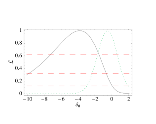
Figure 7: Full line: likelihood for $\delta_{0}$ (marginalized over $\Omega_{\phi}$ and $w_{\phi}$). The horizontal dashed lines give the 68%, 95% and 99% c.l., top to bottom. Dot-dashed line: likelihood for $\delta_{0}$ with the prior $w_{\phi}>-1$.

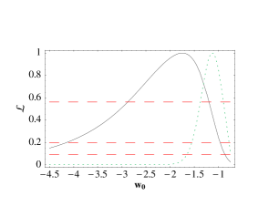
Figure 8: Full line: likelihood for $w_{\phi}$ (marginalized over $\Omega_{\phi}$ and $\delta_{0}$). The horizontal dashed lines give the 68%, 95% and 99% c.l., top to bottom. Dotted line: fixing $\delta_{0}=0$.

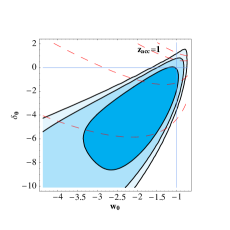
Figure 9: As in Fig. 6, with overimposed the lines of equal acceleration $z_{acc}=0.2,0.4,1,2$ (for $\Omega_{\phi}=0.7$), bottom to top.

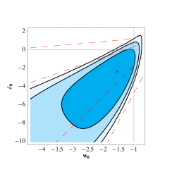
Figure 10: As in Fig. 6 with overimposed the lines of equal age $T=11,12,14,16Gyr$ (assuming $\Omega_{\phi}=0.7$, $h=0.7$) , bottom to top.

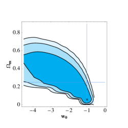
Figure 11: Likelihood for $\Omega_{m},w_{\phi}$ marginalized over $\delta_{0}$ with uniform prior in $(2,-10)$. The vertical and horizontal lines indicate the expected values of $\Omega_{m}$ and $w_{0}$ for a $\Lambda$CDM model.

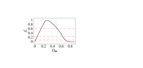
Figure 12: Likelihood for $\Omega_{m}$ marginalized over $\delta_{0},w_{\phi}$. The dotted curve is for uncoupled dark energy ($\delta_{0}=0$).

V Forecasts for future esperiments

V.1 SNAP

There are several project to extend the SNIa dataset both in size and in depth. No doubt they will increase our understanding of the dark energy problem. Here we investigate the potential to constrain the parameters of the interacting model with a SNIa dataset that matches the expectation from the satellite project SNAP.

We generate a random catalog of redshifts and magnitudes of 2000 supernovae from $z=0$ to $z=1.7$, with a r.m.s. magnitude error $\Delta m=0.25$, distributed around a $\Lambda$CDM cosmology with $\Omega_{m0}=0.3,\delta_{0}=0,w_{0}=-1$. The redshift have been assumed uniform in the $z$-range; very likely this is not a good approximation to what SNAP will produce but it is rather difficult at the present stage to predict what the final $z$-distribution will be. It is likely in fact that the statistical significance of the larger number of expected sources at high $z$ will be at least partially reduced by additional uncertainties like lensing effects, redshift errors, spread in the calibration curve etc.. So we preferred to keep the forecast as simple as possible in order not to introduce additional, and not well motivated, parameters.

In Fig. 13 we show the likelihood marginalized over $\Omega_{m0}$. The 68% errors are of order 0.2 for $w_{0}$ and 0.5 for $\delta_{0}$. Such an experiment will therefore be able to increase the precision in $w_{0}$ in $\delta_{0}$ by a factor of five, roughly.

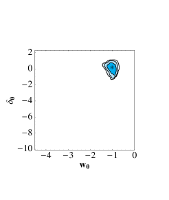
Figure 13: Likelihood contour for a SNAP-like experiment, assuming $\Lambda$CDM ($\Omega_{m}=0.3,\delta_{0}=0,w_{\phi}=-1$) as target cosmology.

V.2 Baryon oscillations

The main limit of the SNIa method is that even satellite experiments like SNAP do not expect to detect a significant number of sources beyond $z=1.7$. It has been suggested that an interesting possibility to probe deeper the cosmic history is the reconstruction of the baryon oscillations in the galaxy power spectrum blake . The method exploits the wiggles in the power spectrum induced by the acoustic oscillations in the baryon-photon plasma before decoupling as a standard ruler. When viewed at different $z$’s, the size of the oscillations map into angular-diameter distances that probe the cosmic geometry just as the luminosity distances of the SNIa.

Here we forecast the constraints on $w_{\phi},\delta_{0}$ by baryon oscillations assuming exactly the same experimental specification of ref. aqg , to which we refer for all the details. To summarize, we evaluated the Fisher matrix of several combined datasets: five deep surveys of 200 $\deg^{2}$ each binned in redshift and centered at $z=0.7,0.9,1.1,1.3,3$, plus a survey similar to the Sloan Digital Sky Survey (SDSS) in the range $z=0-0.3$, plus a cosmic microwave (CMB) experiment similar to the expected performance of the Planck satellite. The five deep surveys are assumed either spectroscopic (negligible error on $z$) or photometric (absolute error $\Delta z=0.04$). The reference cosmology is again $\Lambda$CDM as above. With respect to the method of aqg we marginalize over the growth function.

The results are shown in Fig. 14 for various combinations. The label $z=1$ denotes the combination of the four surveys at $z=0.7-1.3$; $z=3$ denotes the furthest survey. In all cases we include the Fisher matrices of SDSS and CMB. As expected, the deepest data are the most powerful: the dipendence of the angular diameter distance $D$ on $\delta_{0}$ (i.e. $\partial\log D/\partial\log\delta_{0}$) increases by more than a factor of 2 from $z=1$ to $z=3$. Consider first the spectroscopic case (continuous curves): including the survey at $z=3$ pushes down the 68% c.l. errors on $w_{\phi}$ to roughly 0.36 (not far from SNAP forecasts) and to 0.1 the error on $\delta_{0}$, quite better than the SNAP forecasts. Adding the surveys at $z\approx 1$ almost halves the error on $w_{\phi}$ ($\Delta w_{0}\approx 0.22$) while is not particular effective versus the error on $\delta_{0}$. On the other hand, the photometric surveys give constraints $\Delta w_{\phi}\approx 0.6$, $\Delta\delta_{0}\approx 0.5$. Overall, we conclude that the baryon oscillation method at $z\approx 3$ improves upon the SNAP experiment for as concerns $\delta_{0}$, while has a similar efficiency in constraining $w_{\phi}$. In Table I we list all present and future contraints (at 68%) we derived in this paper, bearing in mind that the future experiments have been tested against a $\Lambda$CDM target only: a different target cosmology implies in general different errors.

Method	$\Delta w_{\phi}$	$\Delta\delta_{0}$
Riess et al. (2004) SNIa	$\approx 1$	$\approx 2.5$
Oscillations:$z=1$+$z=3$, spectr.	0.22	0.09
Oscillations:$z=1$+$z=3$, phot.	0.57	0.54
Oscillations:$z=1$, spectr.	0.51	0.81
Oscillations:$z=1$, phot	0.78	2.52
Oscillations:$z=3$, spectr.	0.36	0.10
Oscillations:$z=3$, phot.	0.64	0.66
SNAP	$\approx 0.2$	$\approx 0.5$
Table I

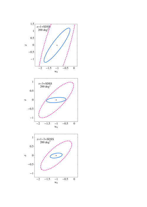
Figure 14: Likelihood contours at 68% estimated from a Fisher matrix analysis of baryon oscillations of several combined surveys. In all plots the inner continuous curve is for spectroscopic surveys, the outer dashed curve for photometric surveys with redshift error 0.04. Top: four survey at $z\approx 1$; middle: survey at $z\approx 3$; bottom: combined surveys at $z\approx 1$ and $z\approx 3$. In all cases, the SDSS survey and the Fisher matrix for a CMB experiment similar to Planck has been included.

VI Conclusions

This paper studied the behavior of a model with three components, baryons, dark matter and dark energy. Contrary to most similar analyses available in literature we included a general phenomenological coupling between dark matter and dark energy specified by a simple but rather general scaling relation. By this extension of dark energy models we have been able to put bounds on the present interaction between the two components or, equivalently, to the rate of change of the dark matter particle mass. Moreover, we can appreciate the extent to which the constraints on such fundamental quantitites as $\Omega_{m}$ and $w_{\phi}$ depend on the assumptions concerning the dark energy interactions.

We obtained several results that we summarize here.

1. We find the constraints on the coupling constant $\delta_{0}$, which can be interpreted as the rate of change of dark matter mass per Hubble time. We obtain $-10<\delta_{0}<-1$ at 95% c.l. and $\delta_{0}<0$ at 99%.

2. We find $-4.2<w_{\phi}<-1$ (95% c.l.). Together with the bounds on $\delta_{0}$ we conclude that the current SN data set favours negatively coupled phantom dark energy. In general, we find that the equation of state correlates with the coupling: positive coupling implies $w_{\phi}<-1$, negative coupling implies phantom energy. Quite remarkably, imposing zero coupling peaks the cosmological constant as preferred value of $w_{\phi}$.

3. Marginalizing over the coupling we derive new bounds on $\Omega_{m0}$. In particular, we find $-4<w_{\phi}<-1$ and $0.05<\Omega_{m0}<0.65$ (95%) . The dark matter density allowed region widens considerably when a nonzero coupling is introduced in the model.

4. We find as best fit a value for the beginning of acceleration $z_{acc}=0.3$ but we cannot exclude earlier acceleration ($z>1$) at more than 95% c.l..

5. We find that the addition of even a small fraction of uncoupled matter, e.g. baryons, modifies profoundly the asymptotic behavior of the model. In particolar, for $\xi<0$ we find models in which the epoch of dark energy dominance (and acceleration) is only temporary. Notice that this occurs for $w_{\phi}$ negative and constant.

6. The ratio of baryons-to-dark matter varies in our model. Depending on $\xi$ it may increse or decrease with time. This may offer new methods of constraining a preferential coupling to dark matter.

7. The big rip that in uncoupled models occurs for $w_{\phi}<-1$ can be prevented if $\delta_{0}>3|w_{\phi}|\Omega_{\phi,0}$; however, these values are unlikely at more than 99% c.l.

Future experiments will constrain the equation of state and the coupling to a much better precision. We find that an experiment with the specification of SNAP might reduce the errors on $\delta_{0},w_{\phi}$ by a factor of five roughly. The method of the baryon oscillations could reduce the error on $\delta_{0}$ by a factor of 25 roughly. Needless to say, these forecasts depend on the exact experimental setting; however, they give a feeling of the expected precision on the dark energy parameters that can be reached a few years from now. Whether the final outcome will show any trace of coupling (or, for that matter, any trace of deviation from a pure cosmological constant) is one of the most exciting question to ask.

- (1) C. Wetterich Nucl. Phys. B., 302, 668 (1988)
- (2) C. Wetterich, Astronomy and Astrophys. 301, 321 (1995).
- (3) T. Damour, G. W. Gibbons and C. Gundlach, Phys. Rev. Lett., 64, 123, (1990)
- (4) L. Amendola Phys. Rev. D62, 043511 (2000)
- (5) Chen X. & Kamionkowsky M. Phys. Rev. D60, 104036 (1999); Uzan J.P., Phys. Rev. D59, 123510 (1999); Baccigalupi C., Perrotta F. & Matarrese S., Phys. Rev. D61, 023507 (2000); Chiba T., Phys. Rev. D60, 083508 (1999); Billyard A.P. & Coley A.A., Phys. Rev. D61, 083503 (2000); O. Bertolami and P. J. Martins, Phys. Rev. D 61, 064007 (2000); Faraoni V., Phys. Rev D62 (2000) 023504; L. P. Chimento, A. S. Jakubi & D. Pavon, Phys. Rev. D62, 063508 (2000), astro-ph/0005070; A. B. Batista, J. C. Fabris and R. de Sa Ribeiro, Gen. Rel. Grav. 33, 1237 (2001); R. Bean and J. Magueijo, Phys.Lett. B517 (2001) 177 ; A.A. Sen & S. Sen MPLA, 16, 1303 (2001), gr-qc/0103098; W. Zimdahl, D. Pavon & L. P. Chimento, Phys.Lett. B521 (2001) 133, astro-ph/0105479; Chiba T., Phys. Rev. D64 103503 (2001) astro-ph/0106550; Esposito-Farese G. & D. Polarsky, Phys. Rev. D63, 063504 (2001) gr-qc/0009034
- (6) A. Bonanno & M. Reuter (2002) Phys. Lett. B 527, 9; P. Teerikorpi, A. Gromov, Yu. Baryshev A&A 407, L9 (2003) astro-ph/0209458; M. Hoffman, astro-ph/0307350; D. Comelli, M. Pietroni and A. Riotto, Phys. Lett. B571, 115 (2003); U. Franca & R. Rosenfeld, Phys. Rev. D69 (2004) 063517, astro-ph/0308149; M. Axenides and K. Dimopoulos, JCAP 0407, (2004) hep-th/0401238; T. Biswas & A. Mazumdar, hep-th/0408026
- (7) S.M. Carroll, Phys. Rev. Lett. 81, 3067 (1998); D. Mota & J. Barrow, Phys.Lett.B581:141,2004 e-Print Archive: astro-ph/0306047
- (8) R. Horvat, JCAP 0208:031 (2002) astro-ph/0007168
- (9) Li M., Wang X., Feng B. & Zhang X., Phys. Rev. D65, 103511 (2002), astro-ph/0112069
- (10) B.A. Gradwohl & Frieman, J. A. 1992 ApJ, 398, 407;
- (11) L. Amendola, C. Quercellini, Phys.Rev.D68:023514, 2003 , astro-ph/0303228
- (12) A. G. Riess et al., ApJ, 607 (2004) 665-687, astro-ph/0402512
- (13) N. Dalal et al., Phys. Rev. Lett., 87, 141302 (2001)
- (14) L. Amendola, M. Gasperini & F. Piazza, JCAP 09 (2004) 007, astro-ph/0407573
- (15) K. Hagiwara et al., Phys. Rev. D66 010001-1 (2002), available at pdg.lbl.gov
- (16) B. Bassett, P. S. Corasaniti & M. Kunz, ApJ, 617 (2004) L1-L4, astro-ph/0407364
- (17) R.R. Caldwell, Phys. Lett. B545, 23 (2002)
- (18) S.W. Allen et. al., Mon.Not.Roy.Astron.Soc. 353 (2004) 457, astro-ph/0405340
- (19) L. Amendola and D. Tocchini-Valentini, astro-ph/0111535, Phys. Rev. D66, 043528 (2002)
- (20) L. Amendola, hep-th/0409224, Phys. Rev. Lett. 93 (2004) 181102
- (21) Eisenstein D.L , Hu W. & Tegmark M., 1999 ApJ 518, 2; Blake C. & Glazebrook K., 2003, ApJ 594, 665 (2003), astro-ph/0301632; Seo H.J. & Eisenstein D., 2003, Ap.J. 598, 720 (2003), astro-ph/0307460; Linder, E. V. 2003, Phys. Rev. D 68, 083504 (2003); Hu W. & Haiman Z., 2003 Phys. Rev. D 68, 063004 (2004), astro-ph/0306053; Cooray A, Huterer D. & Baumann D., Phys. Rev. D69, 027301 (2004)
- (22) L. Amendola, C. Quercellini, E. Giallongo, astro-ph/0404455, MNRAS 357, 429 (2005)