Relations Between Timing Features and Colors in Accreting Millisecond pulsars

Abstract

We have studied the aperiodic X-ray timing and color behavior of the accreting millisecond pulsars SAX J1808.4–3658, XTE J1751–305, XTE J0929–314, and XTE J1814-338 using large data sets obtained with the Rossi X-ray Timing Explorer. We find that the accreting millisecond pulsars have very similar timing properties to the atoll sources and the low luminosity bursters. Based on the correlation of timing and color behavior SAX J1808.4–3658 can be classified as an atoll source, and XTE J0929–314 and XTE J1814–338 are consistent with being atoll sources, but the color behavior of XTE J1751–305 is different. Unlike in other atoll sources the hard color in the extreme island state of XTE J1751–305 is strongly correlated with soft color and intensity, and is not anti-correlated with any of the characteristic frequencies. We found previously, that the frequencies of the variability components of atoll sources follow a universal scheme of correlations. The frequency correlations of the accreting millisecond pulsars are similar, but in the case of SAX J1808.4–3658 and XTE J0929–314 shifted compared to those of the other atoll sources in a way that is most easily described as a shift in upper and lower kilohertz QPO frequency by a factor close to 1.5. Although, we note that the shift in lower kilohertz QPO frequency is based on only one observation for SAX J1808.4–3658. XTE J1751–305 and XTE J1814–338, as well as the low luminosity bursters show no or maybe small shifts.

1 INTRODUCTION

Many low mass X-ray binaries containing a neutron star show kilohertz QPOs, quasi periodic oscillations with frequencies ranging from a few hundred to more than a 1200 Hz. The low frequency ($<200$ Hz) part of the power spectrum taken from their X-ray lightcurves is usually dominated by a broad band-limited noise component. In addition to the band-limited noise several Lorentzian components below 200 Hz are present (see e.g. van Straaten et al. (2002)). These Lorentzians become broader as their characteristic frequency decreases (Psaltis, Belloni, & van der Klis, 1999a; van Straaten et al., 2002). Therefore, several features can, only at high frequencies, be classified as a QPO (traditionally defined by the condition FWHM $<$ centroid frequency/2, see van der Klis, 1995). In addition to these timing features in the persistent emission, 13 sources show millisecond oscillations (270–619 Hz) during thermonuclear X-ray bursts (see Muno, 2004, for a review). Although these burst oscillations show a slight drift, they are thought to be connected with the spin of the neutron star and were the first direct indication that these sources harbour neutron stars with millisecond spins.

Based on the correlated behavior of their timing properties and the behavior of the sources in color-color diagrams, that are used to study their X-ray spectral properties, many of the neutron-star low-mass X-ray binaries are traditionally classified as either “atoll” or “Z” sources (Hasinger & van der Klis, 1989). Recently, Muno et al. (2002) and independently Gierliński & Done (2002a) used the large Rossi X-ray Timing Explorer data sets now available for several of the atoll sources, to show that some of the atoll sources look much more like Z sources when plotted in color-color diagrams than was previously thought. Although the appearances in the color-color diagram of the two classes now is more similar, the classification still holds, as clear differences between the two classes in both timing and color behavior remain (Muno et al., 2002; Barret & Olive, 2002; Olive et al., 2003; van Straaten et al., 2003; Reig et al., 2004). Note, that next to the differences in timing and color behavior there is also a difference in luminosity between the two classes; where the Z sources are all very luminous ($\sim 3\times 10^{38}ergs^{-1}$ Ford et al., 2000), the atoll sources occur over a wide range of luminosities ($10^{36-38}ergs^{-1}$ Ford et al., 2000).

The sources 1E 1724–3045, GS 1826–24, and SLX 1735–269, are all low-luminosity neutron stars that show thermonuclear X-ray bursts. The power spectra of these “low-luminosity bursters” resemble those of the atoll sources in their hard states (Olive et al., 1998; Barret et al., 2000; Belloni, Psaltis, & van der Klis, 2002); they show a broad band-limited noise component and several broad Lorentzian components. However, where the characteristic frequencies of the low-frequency Lorentzians were found to be similar to those in the atoll sources, the characteristic frequency of the highest frequency Lorentzian seemed to be higher (Belloni et al., 2002).

In 1998 the first accreting millisecond pulsar was found with the Rossi X-ray Timing Explorer (RXTE) during an outburst of SAX J1808.4–3658 (Wijnands & van der Klis, 1998a). During this outburst no thermonuclear X-ray bursts were observed and the source did not show kilohertz QPOs above 200 Hz (Wijnands & van der Klis, 1998b). The low frequency power spectrum was very similar to that of the atoll sources (Wijnands & van der Klis, 1998b) and both the atoll sources and SAX J1808.4–3658 followed one relation when the characteristic frequency of a low-frequency Lorentzian was plotted versus that of the band-limited noise (Wijnands & van der Klis, 1999). During a new outburst of SAX J1808.4–3658 in October 2002, kilohertz QPOs (up to 700 Hz) and burst oscillations were observed in an accreting millisecond pulsar for the first time (Wijnands et al., 2003; Chakrabarty et al., 2003). Recently, four additional accreting millisecond pulsars were discovered; XTE J1751–305, XTE J0929–314, XTE J1807–294, and XTE J1814–338 (see Wijnands, 2004, for a observational review). Of these XTE J1807–294 showed kiloherz QPOs (Markwardt, private communication) and XTE J1814–338 showed burst oscillations (Strohmayer et al., 2003).

Here we present an extensive analysis of the aperiodic-timing and color behavior of the accreting millisecond pulsars SAX J1808.4–3658, XTE J1751–305, XTE J0929–314, and XTE J1814–338. We study the correlations between the characteristic frequencies of their various timing features, and compare these with those of four well-studied atoll sources and three low-luminosity bursters. We find, that the accreting millisecond pulsars have very similar timing properties as the atoll sources and the low luminosity bursters, although discrepancies occur for SAX J1808.4–3658 and XTE J0929–314. We also compare the behavior of the accreting millisecond pulsars in the color-color diagrams to that of the atoll sources and find that one pulsar, XTE J1751–305, exhibits unusual behavior while the others act like ordinary atoll sources. In the next section we describe the observations and data analysis. We suggest that readers not interested in the technical details of observations and analysis skip immediately to the results section.

2 OBSERVATIONS AND DATA ANALYSIS

In this work we study four accreting millisecond pulsars: SAX J1808.4–3658, XTE J1751–305, XTE J0929–314, and XTE J1814–338. We also re-analyzed data of Belloni et al. (2002) for the low luminosity bursters 1E 1724–3045, GS 1826–24, and SLX 1735–269 (see §5.1). For the accreting millisecond pulsars we analyzed data from RXTE’s proportional counter array (PCA; for instrument information see Zhang et al., 1993); for SAX J1808.4–3658 we used data from March 11 to May 6, 1998 (the 1998 outburst) and from October 15 to November 26, 2002 (the 2002 outburst), for XTE J1751–305 from April 4 to April 30, 2002, for XTE J0929–314 from May 2 to May 21, 2002, and for XTE J1814–338 from June 8 to August 4, 2003. The data were divided into observations, identified by a unique RXTE observation ID, that cover one to several satellite orbits with $\sim 3000$ s of useful data each. We excluded data for which the angle of the source above the Earth limb is less than 10 degrees or for which the pointing offset is greater then 0.02 degrees. We also excluded type I X-ray bursts. We found 4 bursts in the 2002 outburst of SAX J1808.4–3658 (for results on these bursts see Chakrabarty et al., 2003) for which we excluded 16 s before and 384 s after the onset of each burst, 1 burst in XTE J1751–305 for which we excluded 16 s before and 592 s after the onset of the burst (note that this burst occurred during a weak reflare from April 27–30 for which it is unclear whether it originated from XTE J1751–305, see Markwardt et al. 2002, the burst itself probably originated from GRS 1747–312, which is however ruled out as the source of the reflare, see in’t Zand et al. 2003) and 22 bursts in XTE J1814–338 (for results on these bursts see Strohmayer et al., 2003) for which we excluded 16 s before and 240 s after the onset of each burst, the amount of time excluded depending on the length of the bursts. No bursts were found in XTE J0929–314.

2.1 Color-Color Diagrams

We used the 16–s time-resolution Standard 2 mode to calculate the colors. For each of the PCA’s five PCU detectors separately we calculated a hard color, defined as the count rate in the energy band 9.7$-$16.0 keV divided by that in the 6.0$-$9.7 keV band, and a soft color, defined similarly as 3.5$-$6.0 keV/2.0$-$3.5 keV. For each detector we also calculated the intensity, the count rate in the 2.0$-$16.0 keV band. To obtain the count rates in these exact energy ranges we interpolated linearly between count rates in the PCU channels based on the channel to energy calibration. We subtracted the background contribution in each band using ’pcabackest’ version 3.0, with as input the “Mission-long Faint Model File” if the count rate in the full energy band becomes less than 40 counts s^-1 during an observation (faint data), and otherwise the “Mission-long Bright Model File” (bright data). We averaged up the background-subtracted 16–s count rates to obtain count rates per observation, and we calculated the colors separately for each PCU. An observation spanned between 1 and 30 ks, and within an observation the colors generally varied by 3 to 9 times the 1 $\sigma$ standard deviation of the 16–s colors. For faint data we filtered out data taken within thirty minutes of the peak of the South Atlantic Anomaly and data with high electron contamination.

The voltage settings of the PCUs on board RXTE were changed on three occasions defining the first four RXTE gain epochs. The fifth RXTE gain epoch started when a micro-meteorite created a small hole in the front window of PCU0. In order to correct for the changes in effective detector area between the different RXTE gain epochs and for the gain drifts within these epochs, as well as for the differences in effective area between the PCUs themselves we calculated the colors for each PCU of the Crab nebula, which can supposed to be constant in its colors, in the same manner. We then averaged the 16–s Crab colors and intensity per PCU for each day. For each PCU we divided the obtained color and intensity points per observation by the corresponding Crab values that are closest in time but within the same gain epoch. We then averaged the colors and intensity over all PCUs. Note that starting May 12, 2000, the propane layer on PCU0, which functions as an anti-coincidence shield for charged particles, was lost, defining the beginning of gain epoch 5. Therefore we applied the additional filter recommended by the RXTE science team to PCU0 data from epoch 5.

2.2 Timing

For the Fourier timing analysis we used the 122$-\mu$s time-resolution Event modes and the 0.95$-\mu$s time-resolution Good Xenon modes. We used data from all energy channels. We constructed power spectra per observation (see above) using data segments of 256 s and 1/8192 s time bins such that the lowest available frequency is 1/256 Hz and the Nyquist frequency 4096 Hz; the normalization of Leahy et al. (1983) was used. We subtracted a Poisson noise level using the method of Klein-Wolt et al. (2004), which is built on the analytical function from Zhang et al. (1995). The resulting power spectra were then converted to squared fractional rms. Within the observations the power spectra did not change within the errors. When possible several observations, adjacent in time, and for which the power spectra remain the same, were added up to improve the statistics. These are called groups. Occasionally, several observations, not adjacent in time, for which the power spectra are the same, were added up into groups. The groups for which this was done will be noted in the text (see §3). Before fitting, all frequency bins (generally about 20) containing the pulse spike were removed from the power spectra.

As a fit function we used the multi-Lorentzian function; a sum of Lorentzian components (see e.g. Belloni et al., 2002; van Straaten et al., 2002). Note, that we no longer constrained the Lorentzian (van Straaten et al., 2002, 2003) that fits the band-limited noise component to be zero-centered, but instead let all Lorentzian parameters float. This was motivated by the work of Pottschmidt et al. (2003), who found that for the band-limited noise component in the black hole candidate Cyg X–1, a non zero-centered Lorentzian provided better fits (usually we find a $Q$ significantly larger than zero but $\lesssim 0.3$ for this component, see below). We generally only included those Lorentzians in the fit whose power can be measured to an accuracy of better than 33%. The few exceptions where we deviated from this will be noted in the text (§3). We plot the power spectra in the power times frequency representation ($\nu{\rm P}_{\nu}$), where the power spectral density ${\rm P}_{\nu}$ is multiplied by its Fourier frequency $\nu$. For a multi-Lorentzian fit function this representation helps to visualize a characteristic frequency, $\nu_{\rm max}$, the frequency where each Lorentzian component contributes most of its variance per logarithmic frequency interval, as in $\nu{\rm P}_{\nu}$ the Lorentzian’s maximum occurs at $\nu_{\rm max}$ ($\nu_{\rm max}=\sqrt{\nu_{0}^{2}+\Delta^{2}}$, where $\nu_{0}$ is the centroid and $\Delta$ the HWHM of the Lorentzian; Belloni et al. (2002)). We represent the Lorentzian relative width by $Q$ defined as $\nu_{0}/2\Delta$.

3 RESULTS

We find that three to seven Lorentzian components are needed to fit the power spectra of the millisecond pulsars. All Lorentzian components can be identified in the low mass X-ray binary scheme of Belloni et al. (2002) and van Straaten et al. (2003). In Figure 1 we illustrate the main multi-Lorentzian components of this scheme. Note, that some updates to the scheme based on results of this paper are made (see §5.2). The fit parameters are listed in Tables 1 ($\nu_{\rm max}$), 2 ($Q$), and 3 (fractional rms amplitude). Of the fits for the accreting millisecond pulsars listed in Tables 1, 2, and 3 47% has a $\chi^{2}$/dof below 1.1, 27% has a $\chi^{2}$/dof between 1.1 and 1.3, 23% between 1.3 and 1.7, and 3% (group 4) has $\chi^{2}$/dof = 2.2. The degrees of freedom range between 91 and 142. Note, that the $\chi^{2}$/dof values of the multi-Lorentzian fit function are quite high. However, they are comparable to previous results of this fit function (van Straaten et al., 2002, 2003), and other fit functions tried in previous studies (see Belloni et al., 2002; van Straaten et al., 2002, for a comparison between the multi-Lorentzian fit function and the broken powerlaw fit function ) do not give better results. Note that this is not a problem as here we are only measuring the relevant characteristic frequencies and not trying to find the true model for the power spectra. The fit groups contain data from several RXTE observations. The observation IDs of each fit group are listed in Table 4.

3.1 SAX J1808.4–3658: the 2002 Outburst

In this paragraph we describe the color and timing behavior of SAX J1808.4–3658 during the 2002 outburst as a function of time with the help of Figures 2 and 3. In Figure 2 we show six representative power spectra for the 2002 outburst. In Figure 3 we plot hard color, soft color, intensity (see also Wijnands et al., 2003) and the frequency of one of two timing components (depending on epoch) versus time. We use the terminology of Belloni et al. (2002) and van Straaten et al. (2003) in identifying the timing features (each Lorentzian component is indicated with an L, for example the upper kilohertz QPO is called L_u). In the first group (group 1) a broad L_b at $\sim 10$ Hz, L_h at $\sim 50$ Hz, L_hHz at $\sim 200$ Hz and L_u at $\sim 600$ Hz are observed (see Fig. 2). As the intensity increases to a maximum, both the hard color and the soft color drop to a minimum (Fig. 3). The power spectra (groups 2 and 3) now show L_u at a higher characteristic frequency than in group 1. L_hHz is also present but at a rather high frequency ($\sim 300$ Hz). The low frequency part of the power spectrum is complex; L_h is at a higher frequency than in group 1, and below L_h another low frequency QPO appears that can be identified with L_LF (see §5.2). L_b changes from a broad band-limited noise component into a QPO and L_b2 appears at a lower characteristic frequency (see §5.2). Group 3 is the only group where the lower kilohertz QPO, L_ℓ, can be detected (see also Wijnands et al., 2003). In the fit we fixed the $Q$ value to the value that was found by Wijnands et al. (2003). This was done because with the rebinning used in our fit we only had a few points in this peak. After the maximum, the intensity starts to decrease while the hard color and the soft color increase. The power spectrum of group 4 is similar to that of group 1, showing L_b, L_h, L_hHz, and L_u, at somewhat lower characteristic frequencies. While the intensity continues to decrease, the power spectrum (group 5) still shows these components with $\nu_{b}$, $\nu_{h}$, and $\nu_{u}$ even lower. The characteristic frequency of L_u is now below the spin frequency of 401 Hz. While the intensity keeps decreasing and the soft color starts decreasing, the power spectrum remains about the same for groups 5–8. After that there is a slight increase in intensity accompanied by a decrease in hard color and an increase of $\nu_{b}$, $\nu_{h}$, and $\nu_{u}$ (group 9). Then, while intensity and soft color decrease again, the power spectra of groups 10–15 are very similar to that of group 5. It is not influenced by the break in the intensity and soft color versus time curves that occurs at MJD 52575. In group 15, L_hHz is no longer observed with an upper limit consistent with this component still being present at similar strength (see Table 3). After that no power spectral components are detected until MJD 52578 due to bad statistics (see Wijnands et al., 2003). After MJD 52578 the behavior of the source has changed completely; the intensity fluctuates on time scales of days, and the power spectra show a strong QPO around 1 Hz (see Fig. 2). This behavior is similar to that observed during what appeared to be the end stage of an outburst in 2000 (Wijnands et al., 2001; Wijnands, 2004). The 1 Hz QPOs could not be fitted well with Lorentzians. Instead, several Gaussians were required. In addition to the 1 Hz QPO sometimes another QPO is present at around 30 Hz. As an illustration the centroid frequency of the main Gaussian used to fit the 1 Hz QPO is plotted in the bottom panel of Figure 3. The full behavior of the 1 Hz QPO is beyond the scope of this paper and a detailed analysis of this phenomenon is in progress.

During the 2002 outburst Wijnands et al. (2003) detected a narrow QPO near 410 Hz. To search for these 410 Hz QPOs we created power spectra similar to those of §2.2 but now in the 3–60 keV energy range. This is the same energy range for which Wijnands et al. (2003) found these QPOs. We removed the Poisson level and the pulse spike and fitted the power spectra with the multi-Lorentzian fit function (see also §2.2). To be able to detect the narrow 410 Hz QPO we had to use a finer rebinning than in §2.2. We sometimes had to add several groups, adjacent in time, and for which the power spectra remained the same, to detect the 410 Hz QPO. We find the 410 Hz QPO in group 9 and in the combined groups 5–6, and 10–11. In Figure 4 we plot the combined power spectrum of groups 5–6, 9 and 10–11. The characteristic frequency of the 410 Hz QPO, the frequency difference between the $\sim 401$ Hz pulse spike and the 410 Hz QPO, and L_h are listed in Table 5. We do not detect 410 Hz QPOs during the 1998 outburst.

3.2 SAX J1808.4–3658: the 1998 Outburst

In this paragraph we describe the color and timing behavior of SAX J1808.4–3658 during the 1998 outburst as a function of time with the help of Figures 5 and 6. The 1998 outburst of SAX J1808.4–3658 has been studied extensively previously; the broad-band timing properties where studied by Wijnands & van der Klis (1998b), and the X-ray energy spectrum was studied by Gilfanov et al. (1998), Heindl & Smith (1998), and Gierliński et al. (2002). In group 16 the power spectrum shows L_b at $\sim 2$ Hz, L_h at $\sim 10$ Hz, L_hHz at $\sim 190$ Hz and L_u at $\sim 270$ Hz (see Fig. 5). The characteristic frequencies are all lower than during the 2002 outburst. Note, that the power of L_hHz and L_u could only be measured to an accuracy of better than 50% (and not 33%, see §2.2). However, omitting either one of these components leads to one broad Lorentzian fitting both L_hHz and L_u. For the second observation (at MJD 50916) there is not enough data left to create a power spectrum after the screening criteria have been applied (see §2). After a gap of four days, the intensity and soft color are lower and the hard color is higher. Then, as the intensity and soft color decrease, the power spectrum and hard color remain the same during groups 17–20. The power spectrum (see group 19 in Fig. 5) shows L_b, L_h, and L_u at the lowest characteristic frequencies observed for SAX J1808.4–3658. It also shows L_ℓow at about 30 Hz. In group 21 the intensity, soft and hard color are lower and $\nu_{b}$, $\nu_{h}$, $\nu_{\ell ow}$, and $\nu_{u}$ are higher (see Fig. 5). At MJD 50929, a change of slope in the intensity and soft color curves occurs. This change of slope was also observed during the 2002 outburst (see Fig. 6). Group 22 was fitted with only two Lorentzians, L_b and a broad Lorentzian fitting the higher frequencies. Due to lack of statistics L_h, L_ℓow, and L_u could not be identified.

3.3 XTE J1751–305

In this paragraph we describe the color and timing behavior of XTE J1751–305 during its 2002 outburst as a function of time with the help of Figures 7 and 8. In Figure 7 we show three representative power spectra. In Figure 8 we plot hard color, soft color, intensity and $\nu_{b}$ versus time. Note that in our analysis we subtract the background with RXTE background models (see §2.1). In addition to this there is also a significant background component for XTE J1751–305 due to nearby sources and Galactic diffuse emission (Markwardt et al., 2002). We draw the baseline (the dashed line in the insert of the intensity curve in Fig. 8) through the same observations as was done by Markwardt et al. (2002) and omit the soft and hard color points that are obtained when the source is actually undetected.

In the first observation (group 23) XTE J1751–305 shows L_b at $\sim 1$ Hz, L_h at $\sim 6$ Hz, L_ℓow at $\sim 30$ Hz, and L_u at $\sim 280$ Hz (see Fig. 7). Then with intensity, hard color and soft color decrease (see Fig. 8), group 24 shows the same power spectral components as group 23, but at lower characteristic frequencies. One day later the characteristic frequencies are even lower. Then the power spectrum remains the same for 6 days. To further improve the power spectral statistics we combined these 6 days into group 25. At MJD 52575, the intensity, hard and soft color curves show a change in slope similar to that in the intensity and soft color curves of the 1998 and 2002 outbursts of SAX J1808.4–365 (see §3.1 and 3.2). After the observations that span up group 25, the power spectrum still shows power but the statistics are not sufficient to identify the power spectral components. Between MJD 52380 and MJD 52391 the source is not detected, then a small reflare is observed (see the insert of the intensity curve in Fig. 8), for which it is uncertain whether it is from XTE J1751–305 (Markwardt et al., 2002). The statistics are too low to detect any power spectral components during the reflare.

3.4 XTE J0929–314

In this paragraph we describe the color and timing behavior of XTE J0929–314 during its 2002 outburst with the help of Figures 9 and 10. In Figure 9 we show three representative power spectra. In Figure 10 we plot hard color, soft color, intensity and $\nu_{b}$ versus time. For the first observation (at MJD 52396) there are not enough data left to create a power spectrum after the screening criteria have been applied (see §2). Then, after a gap of seven days, the intensity and soft color are lower and the hard color is higher (see Fig. 10). As the intensity and soft color keep declining the hard color becomes approximately constant. In the next seven days (MJD 52403–52410) the power spectrum shows at low frequencies L_b, L_h, and L_LF/2. L_LF/2 is a narrow QPO ($Q\approx 3$) with a characteristic frequency that varies between 0.6 and 1.3 Hz. At high frequencies the power spectrum shows one broad Lorentzian that probably (see below) fits both L_ℓow and L_u. To improve the statistics at high frequencies we add up the observations with $0.64<\nu_{LF/2}<0.86$ into group 26 and the observations with $0.99<\nu_{LF/2}<1.33$ into group 27. The power spectrum of group 26 shows L_b at $\sim 0.25$ Hz, L_h at $\sim 2$ Hz, and L_LF/2 at $\sim 0.7$ Hz (Fig. 9). At high frequencies L_ℓow and L_u could now be identified. Group 27 is similar to group 26, except that, as mentioned above at high frequencies the fit could not distinguish between L_ℓow and L_u (Fig. 9). After that, from MJD 52411–52428, the power spectra still show power but the statistics are not sufficient to identify the power spectral components. If we add up all observations from MJD 52411–52428 we obtain group 28. This group is similar to group 27, and just as in group 27 the fit does not distinguish between L_ℓow and L_u (Fig. 9). After MJD 52428 the statistics become insufficient and the power spectra no longer show significant power.

3.5 XTE J1814–338

In this paragraph we describe the color and timing behavior of XTE J1814–338 during its 2003 outburst as a function of time with the help of Figures 11 and 12. In Figure 11 we show three representative power spectra. In Figure 12 we plot hard color, soft color, intensity and $\nu_{b}$ versus time. From MJD 52798 to MJD 52825 the power spectra at low frequencies show L_b at $\sim 0.5$ Hz and L_h at $\sim 3$ Hz. The characteristic frequencies vary systematically (see Fig. 12), $\nu_{b}$ between 0.25 and 0.61 Hz, and $\nu_{h}$, which correlates with $\nu_{b}$, between 1.4 and 3.7 Hz. At high frequencies the power spectra are fitted with one broad Lorentzian that probably (see below) fits both L_ℓow and L_u. To improve the statistics at high frequencies we add up the observations with $0.31<\nu_{b}<0.39$ into group 29 and the observations with $0.41<\nu_{b}<0.61$ into group 30. Group 29 shows L_b at $\sim 0.38$ Hz, L_h at $\sim 2.2$ Hz, L_ℓow Hz at $\sim 21$ Hz and L_u at $\sim 190$ Hz (see Fig. 11). It also shows the narrow L_LF/2 at $\sim 0.9$ Hz. Group 30 shows, except for L_LF/2, the same components as group 29 (see Fig. 11). In group 30 all characteristic frequencies are higher; $\nu_{b}\approx 0.5$ Hz, $\nu_{h}\approx 3$ Hz, $\nu_{\ell}\approx 50$ Hz, and $\nu_{u}\approx 220$ Hz. After MJD 52825 the power spectra still show power between MJD 52826 and MJD 52829, but the statistics are not sufficient to identify the power spectral components. After MJD 52830 the statistics become insufficient and the power spectra no longer show significant power.

4 Timing and Colors

Now that we have described and identified all power spectral components in the accreting pulsars SAX J1808.4–365, XTE J1751–305, XTE J0929–314, and XTE J1814–338, we can link the timing properties to the position in the color-color diagram. We can also compare the timing properties and X-ray spectral properties to the classic island and banana states described by Hasinger & van der Klis (1989) and compare with other sources. An addition to the classic states described by Hasinger & van der Klis (1989) is the extreme island state. At the lowest count rates, an extension of the island state is sometimes seen with a harder spectrum and stronger band-limited noise than the ”canonical” island state. The term ”extreme island state” has been used to designate such a state (Prins & van der Klis, 1997; Reig et al., 2000). In Reig et al. (2000) this extreme island state was detached from the ”normal” island state. For 4U 1608–52 (van Straaten et al., 2003) and now here for SAX J1808.4–3658 the change from extreme to ”normal” island state is more gradual, so the question arises where to put the boundary. Here we have used the presence of L_ℓow. In the extreme island state the power spectrum shows L_ℓow and in the island state L_ℓow is absent.

4.1 SAX J1808.4–3658

In Figure 13 we plot the color-color and soft color vs. intensity diagram of both the 2002 and 1998 outburst of SAX J1808.4–365. For the 2002 outburst we only plot observations from before MJD 52578, at which time the behavior of the source changed completely (see §3.1). At the start of the 2002 outburst (group 1) the power spectrum is that of an island state; it shows strong broadband noise with low $\nu_{\rm max}$ and no very low frequency noise (VLFN). Group 2 and 3 show several power spectral characteristics of the lower left banana, the characteristic frequencies are higher, L_ℓ just appears, and the low frequency part of the power spectrum becomes complex. Only the VLFN that is typical for the banana state has not yet appeared. In group 4 the source is back in the island state. After that the source remains in an island state. The characteristic frequencies decrease until group 5, and after that only small changes in the characteristic frequencies occur. During the whole 2002 outburst SAX J1808.4–365 did not go into an extreme island state. In an extreme island state the power spectra show L_b, L_h, L_ℓow and L_u all at very low characteristic frequencies (van Straaten et al., 2003). In 4U 1608–52 (van Straaten et al., 2003) the boundary between island and extreme island state lies at a $\nu_{b}$ of about 2–3 Hz. In the 2002 outburst of SAX J1808.4–3658 L_ℓow was not observed and $\nu_{b}$ was always above 2 Hz. During the 1998 outburst the characteristic frequencies of all components were lower than during the 2002 outburst. In the first group (group 16) of the 1998 outburst SAX J1808.4–365 was in the island state. After that the source was in an extreme island state showing L_ℓow and $\nu_{b}\leq 1$.

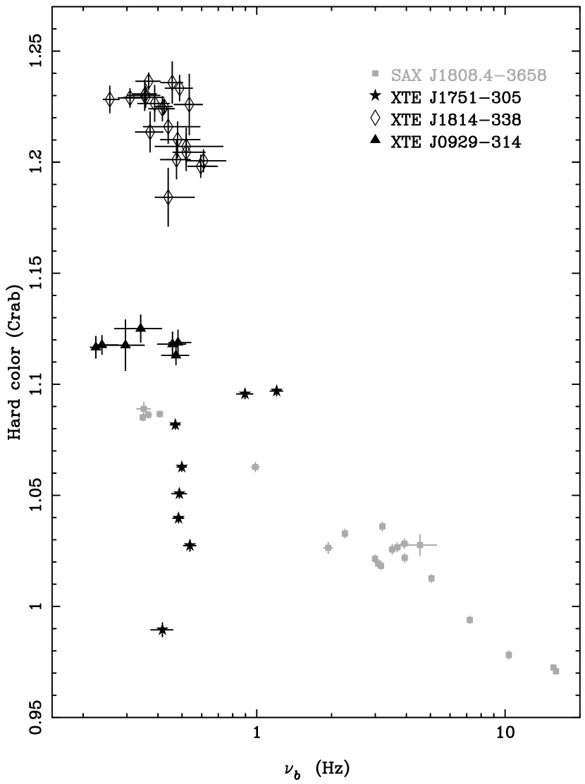
Figure 14: Hard color plotted versus $\nu_{b}$ for SAX J1808.4–3658, XTE J1751–305, XTE J0929–314, and XTE J1814–338. The sources are indicated in the plot.

The determination of the atoll source states based on the power spectral results is in agreement with the positions in the color-color diagram. SAX J1808.4–365 behaves similarly to the atoll sources 4U 1705–44, Aql X–1, and 4U 1608–52 (Muno et al., 2002; Gierliński & Done, 2002a; Barret & Olive, 2002; Olive et al., 2003; van Straaten et al., 2003; Reig et al., 2004) which in the extreme island state show horizontally extended branches in the color-color diagram. At the beginning of the 2002 outburst SAX J1808.4–365 showed a state transition from the island state (group 1) to groups 2 and 3 and back to the island state (group 4). This transition is seen in the color-color diagram as a lowering of the hard and soft color and a slight increase in intensity. At the lowest hard color (groups 2 and 3) the source has almost reached the lower left banana (see above). It seems unlikely that the actual banana branch is reached as the gap between group 2 and 3 is only 3000 s. Then the hard color increases again and the source goes back to an island state. As noted previously (Méndez et al., 1999; van Straaten et al., 2003), hard color appears to be the parameter best correlated to the power spectral characteristics in the island states, and this is confirmed here. During the whole transition, and also in the other groups, the hard color is anti-correlated with the characteristic frequencies of the power spectral components (see Figure 14). This behavior is typical for atoll sources (4U 0614+09, van Straaten et al. 2000; 4U 1728–34, Di Salvo et al. 2001; 4U 1705–44, Olive et al. 2003; 4U 1608–52, van Straaten et al. 2003). Note that compared to other atoll sources the relative change in hard color during the transition is only subtle. For SAX J1808.4–3658 the relative change in hard color is about 5% were it is $\geq 30\%$ for 4U 1728–34 (Di Salvo et al., 2001), 4U 1705–44 (Olive et al., 2003), and 4U 1608–52 (van Straaten et al., 2003). The relative change in soft color is about 10%, comparable to the relative soft color changes for 4U 1728–34, 4U 1705–44, and 4U 1608–52. The behavior after the state transition can be described in the scheme proposed for the atoll sources by van Straaten et al. (2003) (see their figure 12). The source remained in an island state in which the characteristic frequencies are low and hardly change after group 5. Within the island state the soft color changes in correlation with intensity. As the intensity decays the soft color decreases and a horizontally extended island branch appears. Note, that the constant frequencies make this branch very different from the Z source horizontal branch. In other sources horizontally extended branches where only observed in the extreme island state (van Straaten et al., 2003), here we observe the same phenomenon but now in an island state. However, note that the characteristic frequencies in this island state are low and only the absence of L_ℓow distinguish it from an extreme island state (see above) The small changes in characteristic frequency that do occur are accompanied by anti-correlated changes in hard color (see Fig. 14) and show no relation to soft color or intensity. In the 1998 outburst the same phenomenon occurs; in groups 17–20 the power spectra remain in one extreme island state and as the intensity decreases so does the soft color and again a horizontally extended extreme island branch appears. In groups 21–22 the characteristic frequencies are higher and another horizontally extended extreme island branch is formed at a lower hard color. Thus in total three horizontally extended island branches (5–15, 21–22, and 17–20) appear above each other in the left panel of Figure 13, and the frequencies on each of them anti-correlate with hard color. This anti-correlation with hard color also holds between the 1998 and the 2002 outbursts. For a large part (from group 5 of the 2002 outburst) both outbursts cover the same intensity range (see Fig 13). At similar intensities the characteristic frequencies in the 1998 outburst are much lower, while the hard color is higher.

4.2 XTE J1751–305

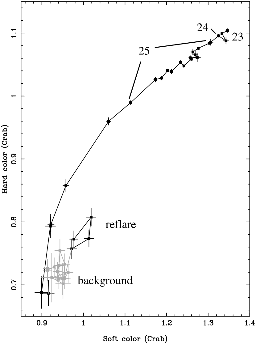
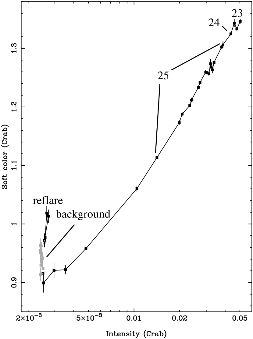
Figure 15: Color-color diagram (left panel) and soft color vs. intensity diagram (right panel) of XTE J1751–305. The black point mark the 2002 outburst and the reflare, the grey points mark the background points that are due to nearby sources and Galactic diffuse emission (see §3.3) The line connects observations that are adjacent in time. The group numbers of the power spectra are indicated. Colors are in units of Crab (see §2).

In Figure 15 we plot the color-color and soft color vs. intensity diagram of XTE J1751–305. The power spectra of XTE J1751–305 show L_b, L_h, L_ℓow and L_u all at low characteristic frequencies. This is typical for an extreme island state. The source stays in an extreme island state during the whole outburst while the characteristic frequencies change between $\nu_{b}=1.2$ and 0.4 Hz. Although the power spectra are typical for those of the extreme island of the atoll sources, the behavior in the color-color diagram is not. During group 25 the characteristic frequencies remain the same. In the atoll sources (and in SAX J1808.4–365, see above) the hard color would then remain the same while the intensity and soft color change in a correlated fashion. This would lead to an extended horizontal branch in the color-color diagram. Here the hard color is not constant but is correlated with intensity in a similar way as the soft color. This correlation between hard color, soft color and intensity exists during the whole outburst. Also, unlike in the atoll sources and SAX J1808.4–3658, no anti-correlation occurs between hard color and the characteristic frequencies of the power spectral components (see Fig. 14). In Figure 15 we also plot the colors of the reflare and those of the background due to nearby sources and Galactic diffuse emission (see §3.3). The points of the reflare do not lie on the the curve of the main outburst, but on an extension of the background. This suggests that the reflare is caused by one of the background sources and not by XTE J1751–305.

4.3 XTE J0929–314

In Figure 16 we plot the color-color and soft color vs. intensity diagram of XTE J0929–314. The filled squares mark group 26, the open diamonds group 27, and the filled stars group 28. The source remains in an extreme island state during the whole outburst, showing L_b, L_h, L_ℓow and L_u all at low characteristic frequencies. The power spectra also show the narrow L_LF/2. This component is also found in 4U 1608–52 (van Straaten et al., 2003) and in XTE J1814–338 (see §4.4), also in the extreme island state. So, the timing behavior is that of the extreme island state of the atoll sources. The behavior in the color-color diagrams is also similar to that of an extreme island state. Within the extreme island state the soft color changes in correlation with intensity. As the intensity decreases the soft color decreases and a horizontally extended island branch appears (see Fig. 16). The hard color and the characteristic frequencies of the power spectral components are not correlated with intensity (and thus soft color). In the atoll sources the hard color is anti-correlated with the characteristic frequencies of the power spectral components. Here that anti-correlation is not evident, but the changes in hard color and characteristic frequencies are only small (see Fig. 14).

4.4 XTE J1814–338

In Figure 17 we plot the color-color and soft color vs. intensity diagram of XTE J1814–338. The filled squares mark group 29, and the open diamonds group 30. The source remains in an extreme island state during that part of the outburst for which power spectral fits could be made. It shows L_b, L_h, L_ℓow and L_u all at low characteristic frequencies. Group 29 also shows the narrow L_LF/2. This component was also found in 4U 1608–52 (van Straaten et al., 2003) and XTE J0929–314 (see §4.3), also in the extreme island state. The timing properties could only be measured in a small range of the color-color diagrams (see Fig. 17). Within this range, the characteristic frequencies, colors and intensity only vary by a small amount, and therefore it is hard to compare this extreme island state of XTE J1814–338 with that of the atoll sources. Within the extreme island state of XTE J1814–338 the soft color (and intensity) does not change enough for the source to draw up a horizontal branch as is often seen in atoll sources in the extreme island state. The range in characteristic frequencies within the extreme island state is too small to observe the anti-correlation between hard color and the characteristic frequencies of the power spectral components that is seen in the atoll sources (see Fig. 14).

5 DISCUSSION

5.1 Correlations of Timing Features

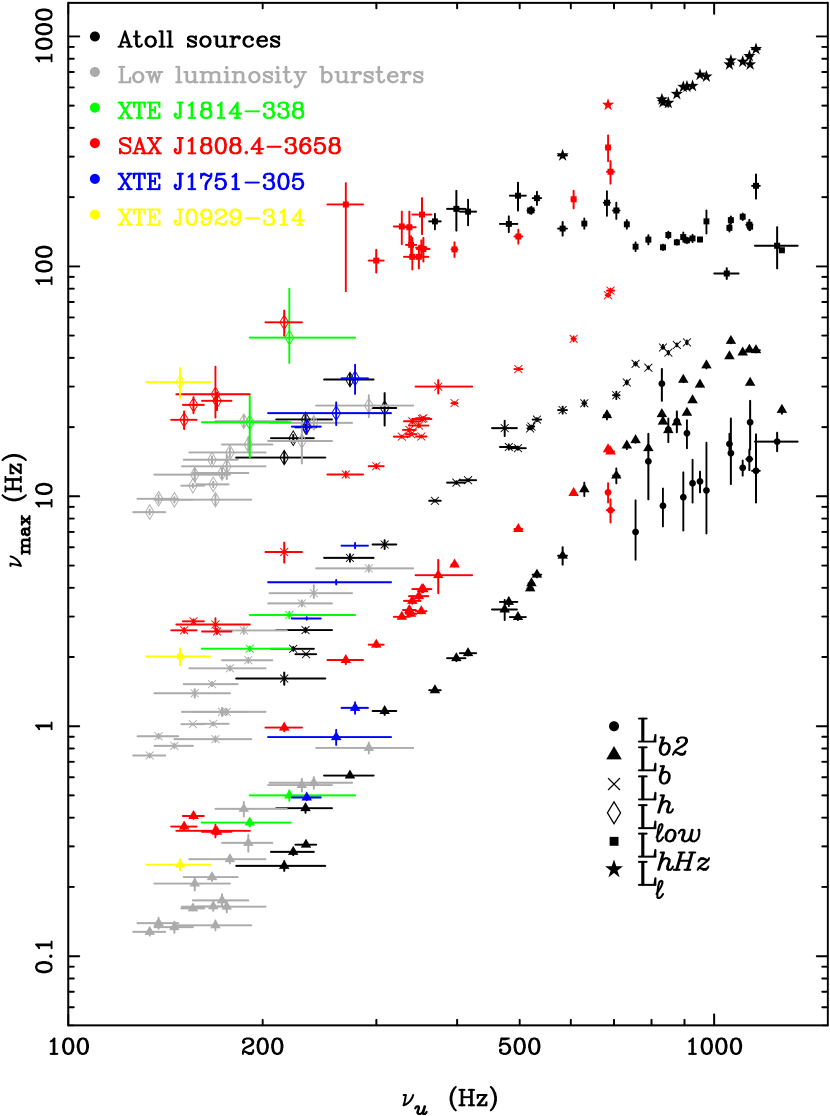
Figure 18: Correlations between the characteristic frequencies ($\equiv\nu_{\rm max}$) of the power spectral components plotted versus $\nu_{u}$. The colored points mark the accreting millisecond pulsars SAX J1808.4–3658 (red), XTE J1751–305 (blue), XTE J0929–314 (yellow), and XTE J1814–338 (green). The black point mark the atoll sources 4U 0614+09, 4U 1608-52, 4U 1728-34, and Aql X–1. The grey point mark the low luminosity bursters 1E 1724–3045, GS 1826–24, and SLX 1735–269. The solid dots mark L_b2, the triangles L_b, the crosses L_h, the squares L_hHz, the stars L_ℓ and the diamonds L_ℓow.

The frequencies of the variability components of the atoll sources, 4U 0614+09, 4U 1608-52, and 4U 1728-34, follow a universal scheme of correlations when plotted versus $\nu_{u}$. In Figure 18 we present such a plot for SAX J1808.4–3658, XTE J1751–305, XTE J0929–314, and XTE J1814–338 (colored points). We also include (black points) results for the atoll sources 4U 0614+09, 4U 1728-34 (van Straaten et al., 2002), 4U 1608-52 (van Straaten et al., 2003), and Aql X–1 (Reig et al., 2004). For Aql X–1 we only include the results for the extreme island state for which $\nu_{u}$ could unambiguously be identified. For 4U 1728-34 we also include a recent result by Migliari, van der Klis, & Fender (2003), where for the first time twin kilohertz QPOs were observed in the island state. As a third group of sources we have included the low luminosity bursters 1E 1724–3045, GS 1826–24, and SLX 1735–269 (grey points) described in Belloni et al. (2002). Belloni et al. (2002) constructed power spectra only up to 512 Hz, which led to an ill-constrained L_u. Here we re-analyze the timing properties of groups C–R of Belloni et al. (2002) using the same method as described in §2.2 (Tables 1, 2, and 3). With 0.0039–4096 Hz power spectra this leads to a much better constrained L_u.

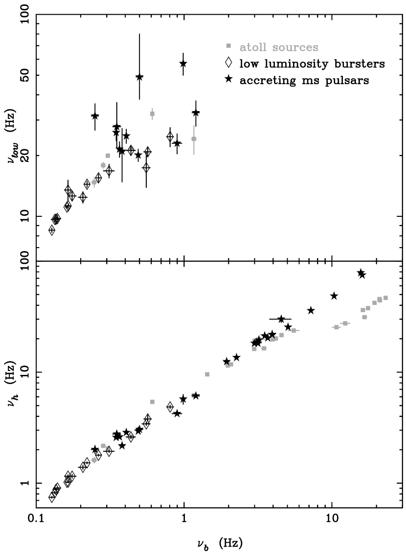
Figure 19: The characteristic frequencies $\nu_{\ell ow}$ (top panel) and $\nu_{h}$ (bottom panel) plotted versus $\nu_{b}$. The filled grey squares mark the atoll sources 4U 0614+09, 4U 1608-52, 4U 1728-34, and Aql X–1, the open black diamonds mark the low luminosity bursters 1E 1724–3045, GS 1826–24, and SLX 1735–269, and the filled black stars mark the accreting millisecond pulsars SAX J1808.4–3658, XTE J1751–305, XTE J0929–314, and XTE J1814–338.

SAX J1808.4–3658 shows similar relations between its characteristic frequencies as the atoll sources do. However, with respect to these sources, the relations of SAX J1808.4–3658 are shifted. XTE J0929–314 shows a similar shift, although this is only based on one power spectrum. XTE J1751–305 and XTE J1814–338 as well as the low luminosity bursters show relations consistent with those of the atoll sources. The shift occurs only between the characteristic frequencies of the low frequency components on the one hand and $\nu_{u}$ (and probably $\nu_{\ell}$) on the other (see below): the mutual relations between the characteristic frequencies of the low frequency components are identical for all sources (see Figure 19).

To determine the actual shift factors between the frequency relations of SAX J1808.4–3658, XTE J0929–314, and those of the atoll sources we consider the $\nu_{i}$ vs. $\nu_{u}$ relations, where $\nu_{i}$ is either $\nu_{b}$, $\nu_{h}$, or $\nu_{\ell ow}$. We only use that part of the relations for which $\nu_{u}<600$ Hz, as the behavior of the low-frequency components above 600 Hz is complex (see also §5.4). We take a $\nu_{i}$ vs. $\nu_{u}$ relation of one source (for example SAX J1808.4–3658) together with that of the atoll sources and perform a power law fit. As our points have errors in both coordinates, we use the FITEXY routine of Press Press & Teukolsky (1992) that performs a straight-line fit to data with errors in both coordinates. We take the logarithm of both $\nu_{i}$ and $\nu_{u}$ so that fitting a straight-line becomes equivalent to fitting a power law. Before fitting we multiply $\nu_{u}$ (or $\nu_{i}$) with a shift factor. We let this shift factor run between 0.1 and 3 with steps of 0.001. The fit with the minimal $\chi^{2}$ then gives the shift factor. The errors in the shift factor use $\Delta\chi^{2}$ = 1.0 (corresponding to a 68% confidence level). In Table 6 we list the shift factors both in $\nu_{u}$ and $\nu_{i}$ for the different relations and sources. Next to the sources that show a clear shift in Figure 18 (SAX J1808.4–3658 and XTE J0929–314) we also include the other millisecond pulsars as well as the low luminosity bursters. We also determine the shift factor for the single $\nu_{\ell}$ observation of SAX J1808.4–3658. We determine the shift factor if only $\nu_{\ell}$ is shifted, and the shift factor if both $\nu_{\ell}$ and $\nu_{u}$ are shifted. For the latter we first multiply $\nu_{u}$ with 1.454, the weighted average of the $\nu_{u}$ shift factors for the $\nu_{b}$, $\nu_{h}$, and $\nu_{\ell ow}$ vs. $\nu_{u}$ relations of SAX J1808.4–3658 (see below).

The shift factors in $\nu_{u}$ for SAX J1808.4–3658 are between 1.4 and 1.5 when determined with the $\nu_{b}$ and $\nu_{h}$ vs. $\nu_{u}$ relation. For the $\nu_{\ell ow}$ vs. $\nu_{u}$ relation the factor is higher, but this is based on fewer points which results in a larger error on the shift factor. From this point on we take the shift in $\nu_{u}$ to be the weighted average of the three which results in 1.454$\pm$0.009. After shifting $\nu_{u}$ with this factor, the additional shift needed for the single $\nu_{\ell}$ point is 1.359, similar to the shift factors found for $\nu_{u}$. For XTE J0929–314 the $\nu_{u}$ shift factors determined with the $\nu_{b}$ and $\nu_{h}$ vs. $\nu_{u}$ relation are similar to those in SAX J1808.4–3658, but note that these results are based on only one point from XTE J0929–314. The $\nu_{\ell ow}$ vs. $\nu_{u}$ relation, just like for SAX J1808.4–3658, gives a higher value but with large error. For some of the other sources small shifts might exist, but unlike for SAX J1808.4–3658 the frequency vs. frequency relations for these sources have up to know only been observed over a small frequency range. The frequency relations should be measured over larger frequency ranges to confirm or reject the idea that small shifts occur.

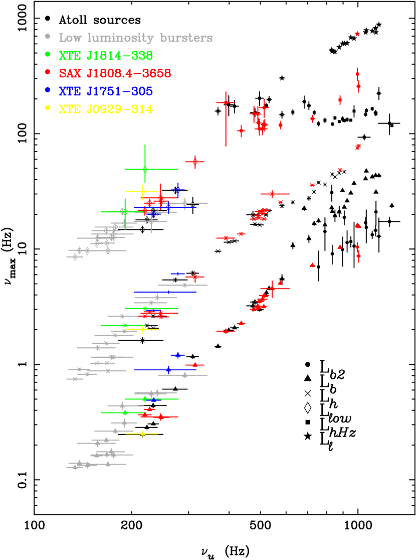
Figure 20: As Figure 18, but with $\nu_{u}$ and $\nu_{\ell}$ of SAX J1808.4–3658 and XTE J0929–314 multiplied by a factor 1.454.

The simplest explanation for this shift is that some physical difference between these sources affects $\nu_{u}$ and $\nu_{\ell}$. To make the relations of SAX J1808.4–3658 and XTE J0929–314 coincide with those of the atoll sources, $\nu_{u}$ and $\nu_{\ell}$ must be multiplied with $\sim 1.5$. In Figure 20 we replot Figure 18, but now with the $\nu_{u}$ and $\nu_{\ell}$ of SAX J1808.4–3658 and XTE J0929–314 multiplied by 1.454. The alternative, that $\nu_{\ell}$ and the characteristic frequencies of all the low frequency components, L_b, L_h, L_ℓow, and the narrow QPOs (see §5.2 for a discussion about the narrow QPOs) are affected is more complex. In this case to make the relations coincide the characteristic frequencies of all the low frequency components have to be multiplied with about 0.35, $\nu_{\ell}$ would have to be multiplied with about 0.8, and $\nu_{hHz}$ would have to remain the same. It is simpler if $\nu_{u}$ and $\nu_{\ell}$ are the shifted frequencies. Note, that the resulting $\chi^{2}$/dof of the power law fits (see Table 6) are independent of whether $\nu_{u}$ or the frequencies of the low frequency components are shifted.

We tried to further test our idea that the shift occurs in $\nu_{u}$ and not in the frequencies of all the low frequency components, by plotting $Q$ versus $\nu_{\rm max}$ for both L_u and L_h (see Figure 21). The $Q_{u}$ vs. $\nu_{u}$ plot showed a shift in $\nu_{u}$ similar to that in Figure 18, while the $Q_{h}$ vs. $\nu_{h}$ plot did not show a clear shift, consistent with the simpler interpretation above. However, the scatter in the $Q$ versus $\nu_{\rm max}$ correlations is much larger than of the frequency-frequency correlations in Figure 18. Neither plots of fractional rms versus $\nu_{\rm max}$ nor linking Figure 18 to the atoll source states led to extra clues.

Might we have wrongly identified the highest frequency Lorentzian component as L_u while it really is L_ℓ? There are a number of arguments against this, all based on similarities with the atoll source class of which SAX J1808.4–3658 seems part (see §4.1). First, L_ℓ was detected together with the component identified as L_u in SAX J1808.4–3658 by Wijnands et al. (2003) (our group 3, see §3.1) when the source was almost in the lower left banana (see §4.1). In group 3 L_ℓ is weak and L_u is strong (see Table 3); this is common behavior for atoll sources when they are almost in the lower left banana (Méndez et al., 2001; van Straaten et al., 2002, 2003). Second, in the island and extreme island states of SAX J1808.4–3658 the component identified as L_u is a strong broad component that is present over a broad frequency range while L_ℓ is not. This is again common behavior for the atoll sources, where L_ℓ was observed in an island state only once, and then as a narrow and weak QPO (Migliari et al., 2003).

5.2 Identifying Timing Features

The frequency relations of the accreting millisecond pulsars and the low luminosity bursters of Figure 18, and especially the shift between the relations of SAX J1808.4–3658 and the atoll sources, provide new clues about the identification of some power spectral components. We assume here that the shift in Figure 18 is a shift in $\nu_{u}$; the conclusions drawn below do not change if we use the alternative, a shift in $\nu_{\ell ow}$, $\nu_{h}$, and $\nu_{b}$ (see §5.1).

The strong, broad highest-frequency Lorentzian in the extreme island state of the atoll sources could previously be identified as either L_u or L_hHz based on its frequency of about 200 Hz. The rms fractional amplitude vs. frequency relations of 4U 0614+09, 4U 1608-52, and 4U 1728-34 gave a hint that this Lorentzian was L_u (van Straaten et al., 2003). Now we observe the same shift in frequency for this Lorentzian as for the component which in other states is unambiguously L_u (see Fig. 18), supporting the conclusion that it is indeed L_u. This conclusion is further strengthened by the results for the low luminosity bursters 1E 1724–3045, GS 1826–24, and SLX 1735–269. These sources, which always have a power spectrum similar to that in the extreme island state of the atoll sources, show a clear correlation between the frequency identified as $\nu_{u}$, and $\nu_{\ell ow}$, $\nu_{h}$, and $\nu_{b}$ (Fig. 18). This would not be expected if this frequency is really $\nu_{hHz}$, as in the atoll sources $\nu_{hHz}$ remains approximately constant while the other frequencies change. Note also that with the addition of the extreme island state results for Aql X–1, the atoll sources now also show these same correlations in the extreme island state (when $\nu_{u}$ is around 200 Hz). So, we identify the broad low frequency features previously reported by Wijnands & van der Klis (1998b) from the 1998 outburst as manifestations of L_u.

The broad L_ℓow component found in the extreme island states of the atoll sources and in the low luminosity bursters has now also been identified in the accreting millisecond pulsars. It was suggested that this component could be identified with the lower kilohertz QPO based on extrapolations of frequency-frequency relations (see Psaltis et al., 1999a; Belloni et al., 2002; van Straaten et al., 2002, 2003), however, it was also noted that it could be a different component (van Straaten et al., 2003). Here we observe that if we make the relations of SAX J1808.4–3658 and XTE J0929–314 coincide with those of the atoll sources by multiplying $\nu_{u}$ with 1.454, the $\nu_{\ell ow}$ vs. $\nu_{u}$ relation of SAX J1808.4–3658 does indeed coincide with the atoll sources one, but the one $\nu_{\ell}$ point of SAX J1808.4–3658 is still offset from the atoll relation. We also have to multiply $\nu_{\ell}$ with a similar factor of about 1.5 to make the L_ℓ point of SAX J1808.4–3658 fall on the atoll relation. If we apply the alternative shift (see §5.1) we have to multiply $\nu_{\ell ow}$ with about 0.35, but $\nu_{\ell}$ with a different factor of about 0.8 to make the relations coincide. Therefore it seems probable that L_ℓow and L_ℓ are different components.

For SAX J1808.4–3658 the characteristic frequency of L_hHz seems to be slightly correlated with the characteristic frequencies of the other components (see Fig. 18). The L_hHz points also seem to lie on an extension of the L_ℓow relation in Figure 18. In the other atoll sources L_ℓow disappears and L_hHz appears when the source goes from the extreme island to the island state. This happens at $\nu_{u}\sim 350$ Hz in Figure 20. It might be that in SAX J1808.4–3658 L_ℓow is present in the island state, but is not detected. It is not detected as a separate component when its characteristic frequency is in the range of $\nu_{hHz}$, causing the correlation of L_hHz with $\nu_{u}$ in Figure 18. However note that the scatter in the L_hHz relation of the atoll sources is large and that a similar scatter in SAX J1808.4–3658 might accidentally cause the correlation of L_hHz with $\nu_{u}$.

In the atoll sources 4U 0614+09, 4U 1608–52, and 4U 1728–34 the behavior of the band-limited noise in the lower left banana state is complex. First, the characteristic frequency of the band-limited noise increases from $\sim 0.3$ to $\sim 15$ Hz. At this stage the band-limited noise is broad. Then at $\sim 15$ Hz this noise component appears to “transform” into a narrow QPO whose frequency increases up to $\sim 50$ Hz, while what appears to be another band-limited noise component appears at lower characteristic frequencies. In our previous papers (van Straaten et al., 2002, 2003) we call the band-limited noise component that becomes a QPO, as well as the QPO it becomes, L_b and the “new” broad band-limited noise appearing at lower frequency L_b2. In SAX J1808.4–3658 the same phenomenon seems to occur in groups 2 and 3. Based on this similar behavior the $\sim 15$ Hz Lorentzian can be identified as L_b and the broad component at $\sim 10$ Hz as L_b2. However, in Figure 20 for $\nu_{u}\gtrsim 600$ Hz the L_b relation of SAX J1808.4–3658 follows the relation of the L_b2 component of the atoll sources. The L_b2 points of SAX J1808.4–3658 fall below that relation. This difference between L_b in SAX J1808.4–3658 and in the other atoll sources can also be seen for $\nu_{b}\gtrsim 10$ Hz in Figure 19. It seems that in this regime the frequency behavior of the band-limited noise in SAX J1808.4–3658 deviates from that in the other atoll sources.

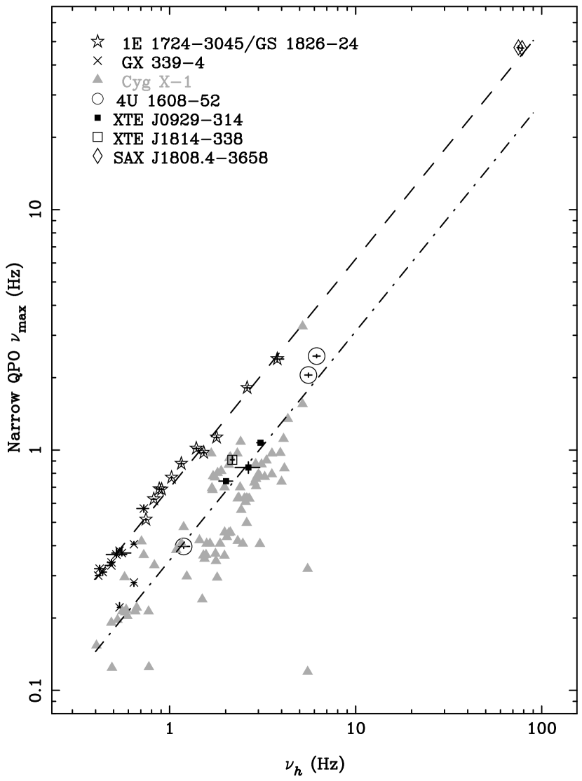
Figure 22: Characteristic frequency of L_h versus that of the narrow low-frequency QPOs that have a $\nu_{\rm max}$ between $\nu_{b}$ and $\nu_{h}$. The sources are indicated in the plot. Note that we use the results of this paper for the low luminosity bursters 1E 1724–3045 and GS 1826–24, which for the low frequencies are in agreement with the results of Belloni et al. (2002) that were used in Figure 13 of van Straaten et al. (2003). The dashed line indicates a power law fit to the $\nu_{LF}$ vs. $\nu_{h}$ relation of the low-luminosity bursters 1E 1724–3045 and GS 1826–24, and the BHC GX 339–4. The dash-dotted line is a power law with a normalization half of that of the dashed line.

In addition to the broad components L_b, L_h, L_ℓow, the low luminosity bursters (Belloni et al., 2002) and the atoll source 4U 1608–52 (van Straaten et al., 2003; Yoshida et al., 1993) show a narrow QPO that has $\nu_{\rm max}$ between $\nu_{b}$ and $\nu_{h}$. The QPO in 4U 1608–52 is not the same as that in the low luminosity bursters (called L_LF) but might be a sub-harmonic (van Straaten et al., 2003). Therefore we will call it L_LF/2. L_LF and L_LF/2 are not only present in neutron star X-ray binaries but could also be identified in the black hole candidate GX 339–4 (Belloni et al., 2002; van Straaten et al., 2003). Also, a narrow QPO found in Cyg X–1 by Pottschmidt et al. (2003) might be L_LF/2 (van Straaten et al., 2003). Until now these QPOs were only found at relatively low frequencies ($<3$ Hz). In this work we find a QPO with a $\nu_{\rm max}$ between $\nu_{b}$ and $\nu_{h}$ at high frequencies ($\approx 47$ Hz) in SAX J1808.4–3658 (groups 2 and 3), and at low frequencies (0.7–1.0 Hz) in XTE J1814–338 (group 29) and XTE J0929–314 (groups 23–25, previously reported by Markwardt et al., 2002). In Figure 22 we plot our results of the SAX J1808.4–3658, XTE J1814–338, and XTE J0929–314 on Figure 13 of van Straaten et al. (2003). Based on the power law relations of Figure 22 we can identify the QPOs in XTE J1814–338 and XTE J0929–314 as L_LF/2 and the QPOs in SAX J1808.4–3658 as L_LF.

5.3 Timing-Color Correlations and States

The timing properties of the accreting millisecond pulsars SAX J1808.4–3658, XTE J1751–305, XTE J0929–314, and XTE J1814–338 are very similar to those of the atoll sources. Also based on its correlated timing and color behavior SAX J1808.4–3658 can be classified as a classical atoll source (see §4.1). In the time span for which timing results could be obtained, XTE J0929–314 and XTE J1814–338 showed little change in power spectra and colors. Therefore it is hard to classify these sources as atoll sources although their correlated timing and color behavior is consistent with that of a typical atoll source (see §4.3 and §4.4). XTE J1751–305 is different from a classical atoll source with respect to the behavior of its hard color (see §3.3). In atoll sources in the island and extreme island states the characteristic frequencies and hard color are anti-correlated with each other, and decoupled from soft color and intensity, which are correlated. The hard color in XTE J1751–305 is instead strongly correlated with soft color and intensity, and is not anti-correlated with any of the characteristic frequencies.

To explain the one-to-one relation between soft color and intensity in an extreme island state of the atoll source 4U 1608–52 van Straaten et al. (2003) used the following scenario: In the extreme island state of 4U 1608–52 the disk is far away from the neutron star and cannot be seen in the PCA energy spectrum; the soft color therefore only depends on the spectral properties of the neutron star (Gierliński & Done, 2002b). As the accretion rate (intensity) increases, the neutron star surface becomes hotter and the soft color increases (van Straaten et al., 2003). This scenario can also be applied to the horizontally extended extreme island state of SAX J1808.4–3658. In an energy spectral study of the 1998 outburst of SAX J1808.4–3658, Gierliński et al. (2002) found that the soft component likely originates from the neutron star surface.

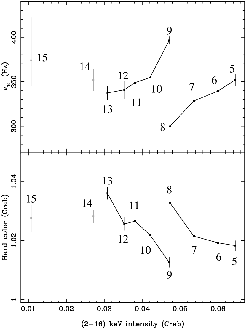
Figure 23: Parallel lines during an island state of SAX J1808.4–3658. The top panel shows the $\nu_{u}$ vs. intensity diagram and the bottom panel the hard color vs. intensity diagram. The group numbers are indicated. The points that span up the parallel tracks are connected by a line.

In the horizontally extended island state branches that are observed in the atoll sources (including SAX J1808.4–3658), contrary to the horizontal branch of Z sources, the timing properties remain similar when the intensity changes. As noted by Olive et al. (2003), this aspect of the behavior can be explained by the scenario of van der Klis (2001) for the parallel track phenomenon in the intensity versus lower kilohertz QPO frequency diagram that occurs in the lower left banana of the atoll sources (see e.g. Méndez, 2000). If we look at these island state branches in SAX J1808.4–3658 during the 2002 outburst (groups 5–15) we observe two parallel tracks (see Figure 23), similar to those in the lower left banana of the atoll sources. This is a further indication that the same physical phenomenon is causing the source to drift between parallel tracks in the lower left banana of the atoll sources and along the island state branches as suggested by van Straaten et al. (2003). We observe one parallel track from group 5 to 8 and the next from group 9 to 13. Both parallel tracks last 4 days; this is longer than the parallel tracks in the lower left bananas which usually last about a day.

5.4 Ingredients for a Physical Model

Currently, to our knowledge, there is no physical model (see van Straaten et al., 2003, for a discussion of models) that explains the mutual relations between the characteristic frequencies of the power spectral features (e.g. Figures 18 and 19). Here we point out some clues that might help to construct such a model. As described above in §5.2, in the lower left banana of the atoll sources (among which we now also classify SAX J1808.4–3658) the behavior of the low frequency components is complex; several timing features, additional to the ones observed in the island states, appear (see e.g. groups 2 and 3 of SAX J1808.4–3658). In Figure 20 this happens at $\nu_{u}\approx 600$ Hz. The Z sources also show a complex low frequency behavior (see Figure 14 in van Straaten et al., 2003), also at high $\nu_{u}$. If $\nu_{u}$ indeed represents the Keplerian frequency at the inner disk radius, a high $\nu_{u}$ means that then the inner disk is close to the neutron star surface, so the more complex behavior might be caused by relativistic or magnetic effects that are stronger close to the neutron star. Note that the power spectra in the extreme island state of some sources also show extra timing features, but these are in the form of weak narrow QPOs that do not dominate the power spectra.

Because of the complex behavior of the low-frequency noise above $\nu_{u}\approx 600$ Hz in Figure 20 we concentrate now on the more simple frequency relations below $\nu_{u}\approx 600$ Hz in Figure 20. The low-frequency relations below $\nu_{u}\approx 600$ Hz can be fitted with power laws (see Table 7). For these fits we use the same method as in §5.1, which uses the FITEXY routine of Press Press & Teukolsky (1992). Note that although the $\chi^{2}$/dof are relatively high, this is not due to systematic deviations from a power law but to scatter around it. The power law indexes of the $\nu_{b}$, $\nu_{h}$, and $\nu_{\ell ow}$ vs. $\nu_{u}$ relations fall in the range 1.8–2.7, progressively steeper towards lower frequency components. The errors on the power law indexes of the L_LF and L_LF/2 relations are large as these relations are only based on a few points, but also these power law indexes are consistent with this picture.

Here we use $\nu_{\rm max}$ as the characteristic frequency. Although $\nu_{\rm max}$ has proven to be of great practical value and may represent a real underlying physical frequency (e.g., the inner frequency of a disk annulus, see Belloni et al., 2002), this is not assured. Two other frequencies, that have physical interpretations in terms of a damped harmonic oscillator, are $\nu_{0}$, the centroid frequency of the Lorentzian and $\nu_{\rm damped}$ (for a definition, see Titarchuk, 2002). These frequencies can be calculated from our fit results $\nu_{\rm max}$ and $Q$ (see van Straaten et al., 2003). Note that using $\nu_{0}$ instead of $\nu_{\rm max}$ does not give further insights in the shift between SAX J1808.4–3658, and the atoll sources (see §5.1). For the narrow Lorentzians the shift factor will be the same as $\nu_{\rm max}$ is approximately equal to $\nu_{0}$, for the broad features $\nu_{0}$ is badly constrained and a shift cannot be determined. For the $\nu_{h,0}$ vs. $\nu_{u,0}$ relation of the atoll sources 4U 0614+09, 4U 1608-52, and 4U 1728-34 van Straaten et al. (2003) found a quadratic relation. A quadratic relation was also found for the $\nu_{h,0}$ vs. $\nu_{u,0}$ relations of several Z sources (Stella & Vietri, 1998; Psaltis et al., 1999b; Jonker et al., 1998; Homan et al., 2002). The relativistic precession model (Stella & Vietri, 1998) predicts a quadratic relation between the Lense-Thirring precession frequency and the Keplerian frequency of the inner disk; $\nu_{LT}=4.4\times 10^{-8}I_{45}M^{-1}\nu_{s}\nu_{K}^{2}$ Hz, where $I_{45}$ is the moment of inertia in units of $10^{45}$ g cm², $M$ is the mass of the neutron star in $M_{\odot}$, and $\nu_{s}$ is the neutron star spin frequency. However, the required $I_{45}/M$ values were too large for L_h to be the fundamental Lense-Thirring precession frequency (Psaltis et al., 1999b). Also the $\nu_{h,0}$ vs. $\nu_{u,0}$ relations coincided for 4U 1728–34 and 4U 1608–52, which is not expected in this interpretation in view of their different spin frequencies (363 Hz and 620 Hz, respectively, assuming burst oscillations happen at the spin frequency). The relation of the frequency difference between the 410 Hz QPO and the $\sim 401$ Hz pulse spike of SAX J1808.4–3658 was found to be consistent with a quadratic relation by Wijnands et al. (2003). We note, that this frequency difference is always about half of $\nu_{h,0}$ (see Table 5).

Although the relations between the characteristic frequencies of the low frequency components and $\nu_{u}$ are different between SAX J1808.4–3658, XTE J0929–314 and the other sources (see §5.1), the mutual relations between the low frequency components are the same for all atoll sources (Fig. 19). The $\nu_{h}$ vs. $\nu_{b}$ relation is even the same for black hole candidates and atoll sources (Wijnands & van der Klis, 1998b; van Straaten et al., 2002). So, the $\nu_{h}$ vs. $\nu_{b}$ relation does not depend on spin, mass, magnetic field, or the presence of a surface. Note, that the frequency range of $\nu_{h}$ and $\nu_{b}$ is about a factor 10 lower for black hole candidates than for neutron star low mass X-ray binaries. Therefore L_b and L_h might be properties of the accretion disk that scale inversely with mass (Wijnands & van der Klis, 1999).

The frequency correlations of SAX J1808.4–3658 and XTE J0929–314 are shifted compared to those of the other sources in a way that is most easily described as a shift in upper and lower kilohertz QPO frequency by about a factor 1.5 (see §5.1). In most models $\nu_{u}$ reflects the Keplerian frequency at the inner edge of the accretion disk (e.g. Miller et al. (1998)). If this is indeed the correct interpretation, then for similar characteristic frequencies of the low frequency components, this inner radius of the disk can somehow get closer to the neutron star surface in the atoll sources, low luminosity bursters, and the accreting millisecond pulsars XTE J1751–305 and XTE J1814–338 than in the accreting millisecond pulsars SAX J1808.4–3658 and XTE J0929–314. It is unclear which physical parameter is the cause of this. In Table 8 we list several characteristic parameters for the accreting millisecond pulsars. There is no obvious relation between the shift and any of the parameters. In particular, there is no relation to spin frequency: SAX J1808.4–3658, and XTE J0929–314 which share one set of frequency relations have spin frequencies of respectively 401 and 185 Hz, and the other sources which share another set of relations have spin frequencies that range from 314 to 620 Hz. Also the magnetic field strength $B$, which may be stronger for the accreting millisecond pulsars than for the atoll sources (see e.g. Wijnands et al., 2003; Strohmayer et al., 2003), is not a good candidate as not all accreting millisecond pulsars show the shift. The fact that the shift occurs by a factor close to $\sim 3/2$ suggests a possible relation with recently proposed parametric resonance models for kilohertz QPOs (e.g. Abramowicz et al., 2003). In these models 2:3 frequency resonances between general relativistic orbital/epicyclic frequencies play a central role. However, similarly to the remarks about inner disk radius above, it is not clear what would set SAX J1808.4–3658 and XTE J0929–314 apart from the other sources.

This work was supported by NWO SPINOZA grant 08–0 to E.P.J. van den Heuvel, by the Netherlands Organization for Scientific Research (NWO), and by the Netherlands Research School for Astronomy (NOVA). This research has made use of data obtained through the High Energy Astrophysics Science Archive Research Center Online Service, provided by the NASA/Goddard Space Flight Center. We would also like to thank the referee, whose comments helped us to improve the paper.

Table 1: Characteristic frequencies of the multi-Lorentzian fit for the accreting millisecond pulsars and low luminosity bursters

Group	Lb	Lb2	Lh	LLF	LLF/2	Lℓow	LhHz	Lℓ	Lu
Number	$\nu_{\rm max}$ (Hz)	$\nu_{\rm max}$ (Hz)	$\nu_{\rm max}$ (Hz)	$\nu_{\rm max}$ (Hz)	$\nu_{\rm max}$ (Hz)	$\nu_{\rm max}$ (Hz)	$\nu_{\rm max}$ (Hz)	$\nu_{\rm max}$ (Hz)	$\nu_{\rm max}$ (Hz)
the accreting millisecond pulsars
SAX J1808.4–3658 (the 2002 outburst)
1	10.34$\pm$0.17	–	48.4$\pm$1.2	–	–	–	196$\pm$17	–	606.0$\pm$4.4
2	15.66$\pm$0.28	8.7$\pm$1.0	78.4$\pm$1.7	47.0$\pm$1.1	–	–	258$\pm$29	–	691.2$\pm$8.7
3	16.02$\pm$0.25	10.4$\pm$1.0	74.9$\pm$1.2	47.28$\pm$0.81	–	–	329$\pm$42	503.6$\pm$5.3	685.1$\pm$5.6
4	7.204$\pm$0.097	–	35.78$\pm$0.37	–	–	–	134.9$\pm$9.3	–	497.6$\pm$6.9
5	3.165$\pm$0.064	–	18.21$\pm$0.19	–	–	–	120.6$\pm$9.1	–	352.1$\pm$6.5
6	3.083$\pm$0.058	–	18.63$\pm$0.20	–	–	–	124$\pm$11	–	339.5$\pm$6.2
7	2.991$\pm$0.049	–	18.17$\pm$0.19	–	–	–	149$\pm$24	–	328.5$\pm$9.2
8	2.264$\pm$0.056	–	13.52$\pm$0.28	–	–	–	106$\pm$12	–	299.9$\pm$8.0
9	5.05$\pm$0.11	–	25.41$\pm$0.28	–	–	–	118.6$\pm$8.7	–	396.4$\pm$4.2
10	3.94$\pm$0.11	–	21.84$\pm$0.32	–	–	–	119$\pm$14	–	354.7$\pm$8.0
11	3.68$\pm$0.11	–	20.30$\pm$0.34	–	–	–	110$\pm$12	–	349$\pm$12
12	3.51$\pm$0.10	–	21.19$\pm$0.44	–	–	–	110$\pm$23	–	341$\pm$10
13	3.205$\pm$0.077	–	19.44$\pm$0.30	–	–	–	148$\pm$25	–	337.5$\pm$7.6
14	3.93$\pm$0.13	–	21.85$\pm$0.34	–	–	–	173$\pm$30	–	352$\pm$12
15	4.54$\pm$0.75	–	30.0$\pm$2.0	–	–	–	–	–	374${}^{+48}_{-29}$
SAX J1808.4–3658 (the 1998 outburst)
16	1.940$\pm$0.077	–	12.44$\pm$0.37	–	–	–	186${}^{+44}_{-108}$	–	269$\pm$17
17	0.407$\pm$0.011	–	2.861$\pm$0.056	–	–	25.0$\pm$2.0	–	–	156.3$\pm$5.8
18	0.366$\pm$0.012	–	2.612$\pm$0.064	–	–	21.5$\pm$1.9	–	–	151.2$\pm$6.8
19	0.3476$\pm$0.0093	–	2.583$\pm$0.065	–	–	26.0$\pm$2.3	–	–	170.0$\pm$8.9
20	0.351$\pm$0.022	–	2.77$\pm$0.18	–	–	27.8$\pm$8.8	–	–	169$\pm$22
21	0.987$\pm$0.035	–	5.72$\pm$0.57	–	–	57.1$\pm$7.1	–	–	216$\pm$14
22	0.969$\pm$0.054	–	–	–	–	–	–	–	–
XTE J1751–305
23	1.202$\pm$0.068	–	6.10$\pm$0.16	–	–	32.6$\pm$4.7	–	–	278$\pm$13
24	0.897$\pm$0.067	–	4.229$\pm$0.092	–	–	23.0$\pm$2.6	–	–	260$\pm$56
25	0.490$\pm$0.013	–	2.942$\pm$0.034	–	–	20.1$\pm$1.4	–	–	234$\pm$12
XTE J0929–314
26	0.250$\pm$0.014	–	2.01$\pm$0.17	–	0.742$\pm$0.013	31.4$\pm$4.7	–	–	149$\pm$17
27	0.463$\pm$0.048	–	3.08$\pm$0.14	–	1.072$\pm$0.022	–	–	–	–
28	0.42$\pm$0.10	–	2.65$\pm$0.40	–	0.846$\pm$0.046	–	–	–	–
XTE J1814–338
29	0.381$\pm$0.015	–	2.173$\pm$0.050	–	0.910$\pm$0.031	21.0$\pm$6.2	–	–	191$\pm$30
30	0.500$\pm$0.026	–	3.048$\pm$0.099	–	–	49${}^{+31}_{-11}$	–	–	220${}^{+58}_{-29}$
the low luminosity bursters
1E 1724–3045
C	0.1614$\pm$0.0034	–	1.0206$\pm$0.0064	–	–	11.12$\pm$0.21	–	–	156.0$\pm$6.3
D	0.555$\pm$0.035	–	3.421$\pm$0.100	–	–	17.4$\pm$3.5	–	–	230$\pm$26
E	0.311$\pm$0.026	–	1.936$\pm$0.048	–	–	16.8$\pm$1.3	–	–	190$\pm$17
F	0.1338$\pm$0.0074	–	0.822$\pm$0.018	0.6246$\pm$0.0049	–	9.65$\pm$0.25	–	–	146$\pm$10
G	0.1392$\pm$0.0075	–	0.905$\pm$0.021	0.6854$\pm$0.0082	–	9.75$\pm$0.37	–	–	138$\pm$10
H	0.1276$\pm$0.0048	–	0.746$\pm$0.015	0.5137$\pm$0.0048	–	8.54$\pm$0.21	–	–	133.7$\pm$7.6
I	0.1362$\pm$0.0066	–	0.879$\pm$0.025	0.688${}^{+0.013}_{-0.007}$	–	9.67$\pm$0.45	–	–	169$\pm$23
J	0.1647$\pm$0.0073	–	1.024$\pm$0.017	0.7676$\pm$0.0091	–	11.27$\pm$0.30	–	–	167.7$\pm$9.4
K	0.207$\pm$0.014	–	1.391$\pm$0.058	1.015$\pm$0.015	–	12.43$\pm$0.80	–	–	157$\pm$21
L	0.175$\pm$0.011	–	1.155$\pm$0.046	0.877$\pm$0.021	–	12.62$\pm$0.61	–	–	173$\pm$17
SLX 1735–269
M	0.1642$\pm$0.0090	–	1.155$\pm$0.033	–	–	13.5$\pm$1.6	–	–	176$\pm$26
GS 1826–24
N	0.264$\pm$0.011	–	1.787$\pm$0.040	1.128$\pm$0.022	–	15.51$\pm$0.67	–	–	178$\pm$24
O	0.2208$\pm$0.0081	–	1.525$\pm$0.031	0.975$\pm$0.020	–	14.42$\pm$0.49	–	–	167$\pm$16
P	0.437$\pm$0.032	–	2.609$\pm$0.084	1.814$\pm$0.039	–	21.2$\pm$1.2	–	–	187$\pm$31
Q	0.805$\pm$0.043	–	4.86$\pm$0.16	–	–	24.8$\pm$2.7	–	–	292$\pm$50
R	0.568$\pm$0.033	–	3.79$\pm$0.31	2.39${}^{+0.11}_{-0.07}$	–	20.87$\pm$0.98	–	–	240$\pm$35

Note. — Listed are the characteristic frequencies ($\equiv\nu_{\rm max}$) of the different Lorentzians used to fit the power spectra of the accreting millisecond pulsars (described in §3) and the low luminosity bursters (see §5.1). The groups of the low luminosity bursters are the same as in Belloni et al. (2002). The quoted errors in $\nu_{\rm max}$ use $\Delta\chi^{2}$ = 1.0 (corresponding to a 68% confidence level).

Table 2: $Q$ values of the multi-Lorentzian fit for the accreting millisecond pulsars and low luminosity bursters

Group	Lb	Lb2	Lh	LLF	LLF/2	Lℓow	LhHz	Lℓ	Lu
Number	$Q$	$Q$	$Q$	$Q$	$Q$	$Q$	$Q$	$Q$	$Q$
the accreting millisecond pulsars
SAX J1808.4–3658 (the 2002 outburst)
1	0.322$\pm$0.013	–	1.03$\pm$0.11	–	–	–	0.60$\pm$0.26	–	5.9$\pm$1.0
2	1.36$\pm$0.20	0.337$\pm$0.034	2.47$\pm$0.57	2.25$\pm$0.37	–	–	0.83$\pm$0.38	–	5.17$\pm$0.95
3	1.35${}^{+0.28}_{-0.18}$	0.272$\pm$0.023	2.66$\pm$0.52	2.38$\pm$0.30	–	–	0.35$\pm$0.18	14.26 (fixed)	5.60$\pm$0.77
4	0.312$\pm$0.012	–	1.195$\pm$0.061	–	–	–	0.43$\pm$0.12	–	2.75$\pm$0.32
5	0.238$\pm$0.015	–	0.813$\pm$0.042	–	–	–	0.281$\pm$0.094	–	2.12$\pm$0.30
6	0.257$\pm$0.014	–	0.807$\pm$0.042	–	–	–	0.28$\pm$0.11	–	2.22$\pm$0.35
7	0.286$\pm$0.014	–	0.914$\pm$0.050	–	–	–	0.03$\pm$0.17	–	3.1${}^{+1.6}_{-0.8}$
8	0.211$\pm$0.017	–	0.642$\pm$0.065	–	–	–	0.18$\pm$0.10	–	1.70$\pm$0.42
9	0.255$\pm$0.016	–	1.136$\pm$0.073	–	–	–	0.32$\pm$0.13	–	4.13$\pm$0.55
10	0.234$\pm$0.019	–	0.890$\pm$0.065	–	–	–	0.30$\pm$0.17	–	2.63$\pm$0.54
11	0.245$\pm$0.021	–	0.949$\pm$0.088	–	–	–	0.34$\pm$0.19	–	2.21${}^{+0.68}_{-0.45}$
12	0.217$\pm$0.021	–	0.875$\pm$0.087	–	–	–	0.35$\pm$0.30	–	2.07${}^{+0.78}_{-0.52}$
13	0.237$\pm$0.017	–	0.891$\pm$0.067	–	–	–	0.22$\pm$0.15	–	2.77${}^{+0.99}_{-0.69}$
14	0.208$\pm$0.022	–	1.085$\pm$0.090	–	–	–	0 (fixed)	–	3.4${}^{+1.3}_{-0.9}$
15	0.13$\pm$0.10	–	0.85$\pm$0.26	–	–	–	–	–	1.47$\pm$0.77
SAX J1808.4–3658 (the 1998 outburst)
16	0.342$\pm$0.035	–	0.489$\pm$0.074	–	–	–	0 (fixed)	–	1.6${}^{+1.6}_{-0.9}$
17	0.186$\pm$0.022	–	0.413$\pm$0.045	–	–	0 (fixed)	–	–	0.362$\pm$0.064
18	0.167$\pm$0.027	–	0.450$\pm$0.061	–	–	0 (fixed)	–	–	0.332$\pm$0.075
19	0.222$\pm$0.021	–	0.240$\pm$0.050	–	–	0 (fixed)	–	–	0.278$\pm$0.077
20	0.309$\pm$0.060	–	0.18$\pm$0.13	–	–	0 (fixed)	–	–	0.26$\pm$0.26
21	0.186$\pm$0.020	–	0 (fixed)	–	–	0.28$\pm$0.16	–	–	0.54$\pm$0.13
22	0.020$\pm$0.045	–	–	–	–	–	–	–	–
XTE J1751–305
23	0.167$\pm$0.033	–	0.70$\pm$0.10	–	–	0.13${}^{+0.23}_{-0.93}$	–	–	1.01$\pm$0.28
24	0.106$\pm$0.043	–	0.787$\pm$0.091	–	–	0.39$\pm$0.20	–	–	0.08${}^{+0.22}_{-0.46}$
25	0.057$\pm$0.018	–	0.724$\pm$0.038	–	–	0 (fixed)	–	–	0.70$\pm$0.12
XTE J0929–314
26	0.76$\pm$0.15	–	0 (fixed)	–	2.67$\pm$0.54	0.47$\pm$0.20	–	–	0.43$\pm$0.21
27	0.382$\pm$0.058	–	0.367$\pm$0.097	–	2.35${}^{+0.77}_{-0.51}$	–	–	–	–
28	0.49${}^{+0.20}_{-0.12}$	–	0.11$\pm$0.21	–	2.0${}^{+1.4}_{-0.7}$	–	–	–	–
XTE J1814–338
29	0.251$\pm$0.026	–	0.581$\pm$0.071	–	3.5${}^{+1.5}_{-1.0}$	0 (fixed)	–	–	0.09${}^{+0.19}_{-0.33}$
30	0.335$\pm$0.037	–	0.290$\pm$0.065	–	–	0.13${}^{+0.20}_{-0.31}$	–	–	0.41${}^{+0.33}_{-0.15}$
the low luminosity bursters
1E 1724–3045
C	0.122$\pm$0.019	–	0.570$\pm$0.016	–	–	0 (fixed)	–	–	0.268$\pm$0.051
D	0.139$\pm$0.044	–	0.653$\pm$0.093	–	–	0 (fixed)	–	–	0.38$\pm$0.15
E	0.117$\pm$0.059	–	0.600$\pm$0.083	–	–	0.10$\pm$0.13	–	–	0.72$\pm$0.20
F	0.135$\pm$0.043	–	0.470$\pm$0.037	7.5${}^{+2.2}_{-1.5}$	–	0.081$\pm$0.042	–	–	0.208$\pm$0.085
G	0.148$\pm$0.044	–	0.512$\pm$0.044	6.6${}^{+8.9}_{-2.2}$	–	0.036$\pm$0.068	–	–	0.30$\pm$0.12
H	0 (fixed)	–	0.535$\pm$0.032	6.21$\pm$0.82	–	0 (fixed)	–	–	0.229$\pm$0.078
I	0.210$\pm$0.046	–	0.479$\pm$0.057	7${}^{+17}_{-3}$	–	0.033$\pm$0.085	–	–	0.11${}^{+0.15}_{-0.25}$
J	0.083$\pm$0.036	–	0.553$\pm$0.031	7.1$\pm$1.3	–	0 (fixed)	–	–	0.375$\pm$0.078
K	0.122$\pm$0.049	–	0.505$\pm$0.064	4.4${}^{+1.6}_{-1.1}$	–	0.07$\pm$0.12	–	–	0.25$\pm$0.16
L	0.111$\pm$0.045	–	0.491$\pm$0.050	3.2${}^{+1.6}_{-0.9}$	–	0 (fixed)	–	–	0.30$\pm$0.13
SLX 1735–269
M	0.040$\pm$0.042	–	0.457$\pm$0.061	–	–	0 (fixed)	–	–	0.33$\pm$0.16
GS 1826–24
N	0.050$\pm$0.029	–	0.562$\pm$0.050	7.1$\pm$2.9	–	0.082$\pm$0.075	–	–	0.38$\pm$0.23
O	0.139$\pm$0.028	–	0.486$\pm$0.037	6.2${}^{+2.5}_{-1.5}$	–	0 (fixed)	–	–	0.47$\pm$0.14
P	0.049$\pm$0.045	–	0.69$\pm$0.10	5.6${}^{+2.6}_{-1.3}$	–	0.05$\pm$0.10	–	–	1.4 ${}^{+1.3}_{-0.6}$
Q	0.133$\pm$0.040	–	0.76$\pm$0.12	–	–	0.29$\pm$0.20	–	–	0.82$\pm$0.44
R	0.017$\pm$0.043	–	0.684$\pm$0.095	2.9$\pm$1.1	–	0.43$\pm$0.11	–	–	0.46$\pm$0.20

Note. — Listed are the $Q$ values ($\equiv\nu_{\rm 0}/2\Delta$) of the different Lorentzians used to fit the power spectra of the accreting millisecond pulsars (described in §3) and the low luminosity bursters (see §5.1). The groups of the low luminosity bursters are the same as in Belloni et al. (2002). The quoted errors in $Q$ use $\Delta\chi^{2}$ = 1.0 (corresponding to a 68% confidence level).

Table 3: Integrated fractional rms of the multi-Lorentzian fit for the accreting millisecond pulsars and low luminosity bursters

Group	Lb	Lb2	Lh	LLF	LLF/2	Lℓow	LhHz	Lℓ	Lu
	rms (%)	rms (%)	rms (%)	rms (%)	rms (%)	rms (%)	rms (%)	rms (%)	rms (%)
the accreting millisecond pulsars
SAX J1808.4–3658 (the 2002 outburst)
1	17.05$\pm$0.14	–	11.78$\pm$0.65	–	–	–	10.2$\pm$1.1	–	8.92$\pm$0.50
2	8.68$\pm$0.91	10.13$\pm$0.85	6.96$\pm$0.75	6.87$\pm$0.57	–	–	7.98$\pm$0.98	–	8.32$\pm$0.57
3	8.7$\pm$1.2	12.55$\pm$0.96	6.79$\pm$0.66	7.17$\pm$0.49	–	–	11.66$\pm$0.95	2.94$\pm$0.48	8.78$\pm$0.58
4	16.61$\pm$0.11	–	13.94$\pm$0.38	–	–	–	12.43$\pm$0.72	–	10.87$\pm$0.49
5	15.40$\pm$0.15	–	15.71$\pm$0.35	–	–	–	14.99$\pm$0.78	–	10.84$\pm$0.74
6	15.11$\pm$0.14	–	15.73$\pm$0.35	–	–	–	14.71$\pm$0.87	–	10.76$\pm$0.82
7	15.23$\pm$0.12	–	15.25$\pm$0.40	–	–	–	17.3$\pm$1.3	–	8.8$\pm$1.5
8	16.23$\pm$0.20	–	14.21$\pm$0.59	–	–	–	17.0$\pm$1.1	–	11.4$\pm$1.3
9	16.03$\pm$0.16	–	14.58$\pm$0.48	–	–	–	14.39$\pm$0.87	–	10.29$\pm$0.57
10	15.30$\pm$0.21	–	16.11$\pm$0.56	–	–	–	14.1$\pm$1.2	–	10.67$\pm$0.99
11	15.56$\pm$0.22	–	15.58$\pm$0.67	–	–	–	14.5$\pm$1.4	–	10.9$\pm$1.2
12	15.67$\pm$0.22	–	16.03$\pm$0.84	–	–	–	13.9$\pm$2.2	–	11.9$\pm$1.6
13	16.37$\pm$0.18	–	15.60$\pm$0.51	–	–	–	16.5$\pm$1.5	–	10.7$\pm$1.5
14	16.14$\pm$0.23	–	14.28$\pm$0.48	–	–	–	19.22$\pm$0.93	–	9.0$\pm$1.4
15	15.4$\pm$1.1	–	17.1$\pm$1.5	–	–	–	$<16.0$	–	19.5$\pm$2.8
SAX J1808.4–3658 (the 1998 outburst)
16	15.32$\pm$0.38	–	16.09$\pm$0.61	–	–	–	18.7${}^{+2.1}_{-5.0}$	–	10.1${}^{+9.5}_{-2.6}$
17	19.76$\pm$0.25	–	15.85$\pm$0.49	–	–	18.14$\pm$0.46	–	–	19.85$\pm$0.68
18	20.85$\pm$0.31	–	15.34$\pm$0.64	–	–	19.04$\pm$0.51	–	–	20.58$\pm$0.79
19	20.26$\pm$0.31	–	17.33$\pm$0.60	–	–	19.04$\pm$0.55	–	–	19.65$\pm$0.85
20	18.83$\pm$0.82	–	18.0$\pm$1.5	–	–	18.1$\pm$2.0	–	–	20.8$\pm$2.6
21	16.33$\pm$0.39	–	16.53$\pm$0.35	–	–	15.8$\pm$2.0	–	–	17.3$\pm$1.6
22	25.08$\pm$0.48	–	–	–	–	–	–	–	–
XTE J1751–305
23	10.70$\pm$0.29	–	12.0${}^{+0.8}_{-1.2}$	–	–	11.2$\pm$2.5	–	–	12.2$\pm$1.1
24	11.89$\pm$0.39	–	12.37$\pm$0.65	–	–	10.9$\pm$1.5	–	–	15.3$\pm$1.5
25	12.53$\pm$0.13	–	12.05$\pm$0.26	–	–	14.57$\pm$0.23	–	–	13.49$\pm$0.57
XTE J0929–314
26	5.36$\pm$0.44	–	15.99$\pm$0.25	–	5.00$\pm$0.49	13.3$\pm$2.1	–	–	18.8$\pm$2.0
27	8.13$\pm$0.52	–	12.66$\pm$0.61	–	5.23$\pm$0.73	–	–	–	–
28	7.1$\pm$1.6	–	12.6$\pm$1.2	–	5.0${}^{+1.8}_{-1.2}$	–	–	–	–
XTE J1814–338
29	11.82$\pm$0.28	–	13.92$\pm$0.65	–	2.89$\pm$0.58	15.4$\pm$1.9	–	–	22.0$\pm$2.1
30	9.83$\pm$0.46	–	15.81$\pm$0.705	–	–	16.5${}^{+5.7}_{-2.8}$	–	–	19.2${}^{+2.4}_{-4.5}$
the low luminosity bursters
1E 1724–3045
C	14.16$\pm$0.14	–	16.06$\pm$0.14	–	–	18.201$\pm$0.098	–	–	13.87$\pm$0.30
D	12.00$\pm$0.33	–	12.20$\pm$0.74	–	–	12.24$\pm$0.52	–	–	14.37$\pm$0.93
E	11.87$\pm$0.42	–	13.57$\pm$0.69	–	–	14.14$\pm$0.79	–	–	11.73$\pm$0.92
F	14.37$\pm$0.39	–	16.46$\pm$0.46	3.25$\pm$0.31	–	18.50$\pm$0.40	–	–	14.75$\pm$0.56
G	14.32$\pm$0.36	–	16.27$\pm$0.49	2.51${}^{+0.66}_{-0.32}$	–	18.20$\pm$0.57	–	–	14.13$\pm$0.76
H	16.07$\pm$0.24	–	15.15$\pm$0.35	4.21$\pm$0.31	–	19.33$\pm$0.13	–	–	13.70$\pm$0.41
I	14.12$\pm$0.38	–	16.00$\pm$0.55	3.29${}^{+0.74}_{-0.46}$	–	18.47${}^{+0.65}_{-0.93}$	–	–	14.3$\pm$1.0
J	14.71$\pm$0.29	–	15.42$\pm$0.34	3.32$\pm$0.34	–	18.39$\pm$0.13	–	–	13.65$\pm$0.45
K	14.29$\pm$0.44	–	15.36$\pm$0.74	4.47${}^{+0.88}_{-0.61}$	–	16.71$\pm$0.99	–	–	14.0$\pm$1.1
L	14.15$\pm$0.39	–	15.38$\pm$0.59	4.7${}^{+1.3}_{-0.8}$	–	18.03$\pm$0.24	–	–	13.39$\pm$0.71
SLX 1735–269
M	9.95$\pm$0.24	–	9.96$\pm$0.38	–	–	12.37$\pm$0.41	–	–	12.78$\pm$0.94
GS 1826–24
N	12.66$\pm$0.21	–	11.90$\pm$0.45	1.92$\pm$0.52	–	15.28$\pm$0.61	–	–	9.01$\pm$0.99
O	14.28$\pm$0.24	–	14.20$\pm$0.36	2.38$\pm$0.39	–	18.60$\pm$0.16	–	–	10.27$\pm$0.63
P	14.14$\pm$0.41	–	12.73$\pm$0.88	3.15$\pm$0.57	–	17.24$\pm$0.66	–	–	7.5$\pm$1.4
Q	13.61$\pm$0.31	–	13.36$\pm$1.00	–	–	13.2${}^{+1.5}_{-1.1}$	–	–	10.0$\pm$1.5
R	14.25$\pm$0.34	–	13.02$\pm$0.84	4.6${}^{+1.8}_{-0.7}$	–	13.75$\pm$0.78	–	–	12.6$\pm$1.1

Note. — Listed are the values of the integrated fractional rms (over the full PCA energy band) of the different Lorentzians used to fit the power spectra of the accreting millisecond pulsars (described in §3) and the low luminosity bursters (see §5.1). The groups of the low luminosity bursters are the same as in Belloni et al. (2002). The quoted errors in the rms use $\Delta\chi^{2}$ = 1.0 (corresponding to a 68% confidence level).

Table 4: RXTE observation IDs of the fit groups

Group	RXTE observation IDs
1	C-04-00, A-01-000
2	A-01-00, A-01-03, A-01-04
3	A-01-01
4	A-01-020, A-01-02
5	A-02-01, A-02-000, A-02-00
6	A-02-02, A-02-03, A-02-04
7	A-02-05, A-02-06, A-02-07
8	A-02-10, A-02-08
9	A-02-20, A-02-09, A-02-19, A-02-23
10	A-02-21, A-02-11, A-02-18, A-02-12, A-02-22
11	A-02-13, A-02-15, A-02-14, A-02-16
12	A-02-17, A-03-000, A-03-00, A-03-04, A-03-05
13	A-03-06, A-03-07, A-03-010, A-03-01, A-03-08, A-03-09, A-03-10, A-03-11
14	A-03-12, A-03-13, A-03-02, A-03-14, A-03-03, C-05-00, B-01-04
15	B-01-000, B-01-00
16	D-01-03S
17	D-03-00, D-04-00
18	D-05-00
19	D-06-01, D-06-000, D-06-00
20	D-07-00
21	D-08-00, D-09-01, D-09-02, D-09-03, D-09-04
22	D-09-00, D-10-02, D-10-01, D-10-00
23	E-01-00, F-01-00, E-02-00
24	F-02-00
25	F-03-01, F-03-00, F-04-00 F-05-03, F-05-02, F-05-01, F-05-04, F-05-000, F-05-00, F-06-00,
	F-06-01, F-07-00, F-07-01, F-08-000, F-08-00, F-09-000
26	G-03-01, G-03-00, G-04-00, G-04-01, G-05-01, G-07-01
27	G-02-00, G-02-01, G-06-01, G-06-00, G-05-00, G-07-00
28	G-08-00, G-08-01, G-08-02, G-08-03, G-08-04, G-08-05, G-08-06, G-09-00, G-09-01, G-09-02,
	G-10-00, G-10-01, G-10-02, G-10-03, G-10-04, G-11-00, G-12-00, G-12-01, G-12-02
29	H-01-01, H-01-02, H-01-03, H-01-04, H-01-05, H-01-06, H-02-04, H-02-05, H-03-12, H-03-13,
	H-03-000, H-03-00, H-03-01, H-03-03, H-03-04, H-03-05, H-03-02, H-03-06, H-03-07
30	H-01-07, H-01-08, H-01-09, H-02-01, H-02-00, H-02-03, H-02-02, H-02-06, H-02-07, H-02-09,
	H-02-08, H-03-08, H-03-09, H-03-10, H-03-11, H-04-07, H-04-00, H-04-01, H-04-02, H-04-08,
	H-04-03, H-04-04, H-04-05, H-04-09, H-04-06, H-05-00, H-05-01

Note. — Listed are RXTE observation IDs of each fit group. The letters stand for part of the observation ID; A = 70080-01, B = 70080-02, C = 70080-03, D = 30411-01, E = 70134-03, F = 70131-01, G = 70096-03, and H = 80418-01.

Table 5: Characteristic frequencies of the 410 Hz QPO

Groups	410 Hz QPO	$\nu_{\rm 410}-\nu_{\rm pulse}$	Lh
	$\nu_{\rm max}$ (Hz)	(Hz)	$\nu_{\rm max}$ (Hz)	$\nu_{0}$ (Hz)
5–6	409.2${}^{+0.6}_{-1.0}$	8.3${}^{+0.6}_{-1.0}$	18.67$\pm$0.15	16.81$\pm$0.13
9	413.41$\pm$0.30	12.47$\pm$0.30	25.55$\pm$0.29	23.41$\pm$0.26
10–11	409.3$\pm$1.7	8.36$\pm$1.7	20.95$\pm$0.24	18.54$\pm$0.21

Note. — Listed are the characteristic frequency ($\nu_{\rm max}$) of the 410 Hz QPO, the frequency difference between the $\sim 401$ Hz pulse spike ($\nu_{\rm pulse}$) and the 410 Hz QPO ($\nu_{\rm 410}-\nu_{\rm pulse}$). Also listed are the $\nu_{\rm max}$ and $\nu_{0}$ of L_h. $\nu_{0}$ is the centroid frequency of the Lorentzian and can be obtained from our fit parameters $\nu_{\rm max}$ and $Q$ as $\nu_{0}=2\nu_{\rm max}Q/\sqrt{4Q^{2}+1}$. For the 410 Hz QPO $\nu_{\rm max}=\nu_{0}$ as $Q$ is between 50 and 100.

Table 6: Shift factors

$\nu_{i}$	$\nu_{u}$ shift factor	$\nu_{i}$ shift factor	$\chi^{2}$/dof
	($\nu_{u}\times$ factor)	($\nu_{i}\times$ factor)
SAX J1808.4–3658
$\nu_{b}$	1.420$\pm$0.013	0.355$\pm$0.013	35.4/31
$\nu_{h}$	1.481$\pm$0.013	0.375$\pm$0.011	54.5/31
$\nu_{\ell ow}$	1.653$\pm$0.073	0.334$\pm$0.061	7.8/9
$\nu_{\ell}$	–	1.359$\pm$0.021	183.8/15
$\nu_{\ell}$	–	0.804$\pm$0.015	183.8/15
XTE J0929–314
$\nu_{b}$	1.40$\pm$0.16	0.35$\pm$0.13	15.8/15
$\nu_{h}$	1.41$\pm$0.16	0.42$\pm$0.13	30.1/15
$\nu_{\ell ow}$	2.03$\pm$0.30	0.283$\pm$0.090	5.5/5
XTE J1751–305
$\nu_{b}$	1.188$\pm$0.045	0.585$\pm$0.073	18.6/17
$\nu_{h}$	1.112$\pm$0.042	0.763$\pm$0.076	32.9/17
$\nu_{\ell ow}$	1.036$\pm$0.058	0.93$\pm$0.10	6.3/7
XTE J1814–338
$\nu_{b}$	1.23$\pm$0.14	0.53$\pm$0.19	15.8/16
$\nu_{h}$	1.13$\pm$0.13	0.73$\pm$0.22	30.1/16
$\nu_{\ell ow}$	1.42$\pm$0.24	0.52$\pm$0.16	6.5/6
1E 1724–3045
$\nu_{b}$	1.167$\pm$0.043	0.622$\pm$0.076	22.2/24
$\nu_{h}$	1.037$\pm$0.040	0.915$\pm$0.091	36.7/24
$\nu_{\ell ow}$	1.051$\pm$0.077	0.92$\pm$0.12	9.7/14
SLX 1735–269
$\nu_{b}$	1.04$\pm$0.15	0.90$\pm$0.40	15.8/15
$\nu_{h}$	0.96$\pm$0.14	1.11$\pm$0.41	30.1/15
$\nu_{\ell ow}$	1.07$\pm$0.18	0.88$\pm$0.27	5.5/5
GS 1826–24
$\nu_{b}$	1.195$\pm$0.071	0.58$\pm$0.11	17.4/19
$\nu_{h}$	1.134$\pm$0.067	0.73$\pm$0.11	31.1/19
$\nu_{\ell ow}$	1.117$\pm$0.075	0.83$\pm$0.11	9.1/9

Note. — Shift factors between the frequency relations of the listed sources and the atoll sources (see §5.1). The errors in the shift factor use $\Delta\chi^{2}$ = 1.0.

Table 7: Power law fits to the frequency relations

Component	Index	Normalization	$\chi^{2}$/dof
Lb	2.724$\pm$0.038	$1.49(\pm 0.34)\times 10^{-7}$	152/53
Lh	2.439$\pm$0.030	$4.62(\pm 0.85)\times 10^{-6}$	89/53
Lℓow	1.81$\pm$0.11	$1.15(\pm 0.66)\times 10^{-3}$	34/31
LLF	3.00$\pm$0.63	$2.0(\pm 6.9)\times 10^{-7}$	6/9
LLF/2	3.13$\pm$0.84	$4(\pm 22)\times 10^{-8}$	1.7/1

Note. — Listed are the index, the normalization and the $\chi^{2}$/dof of power law fits to the $\nu_{\rm max}$ versus $\nu_{u}$ relations in Figure 20. Only the data below about $\nu_{u}\approx 600$ Hz is included in the fit.

Table 8: Characteristic parameters for the accreting millisecond pulsars

Source	$\nu_{spin}$	Porb	Bursts	Shift factor	References
SAX J1808.4–3658	401 Hz	2 hr	Y	$\sim 1.5$	a, b, c, d
XTE J0929–314	185 Hz	44 min	N	$\sim 1.5$	e
XTE J1751–305	435 Hz	42 min	N	$\sim 1$	f
XTE J1814–338	314 Hz	4.3 hr	Y	$\sim 1$	g, h, i

Note. — Listed are the source name, the spin frequency, $\nu_{spin}$, the orbital period, P_orb, whether or not the source has shown type I X-ray bursts, and the shift factor that has to be applied to $\nu_{u}$ to make the relations coincide with those of the atoll sources (see §5.1).

Figure 1: The multi-Lorentzian components of the low mass X-ray binary scheme of Belloni et al. (2002) and van Straaten et al. (2003). The states in which the components occur are indicated; lower left banana (LLB), island state (IS), and extreme island state (EIS). Note that L_LF and L_LF/2 are not shown. They generally occur in the extreme island state as a narrow QPO with a frequency between that of L_b and L_h.

Figure 2: Six representative power spectra and fit functions in the power spectral density times frequency representation for the 2002 outburst of SAX J1808.4–3658. The different lines in the first 5 panels mark the individual Lorentzian components of the fit that are also indicated in the plots. The dashed lines in the sixth panel mark the Gaussian components of the fit, the dotted lines mark the Lorentzian components. The arrows indicate the 401 Hz pulsar spike that was excluded during the fit. The group numbers are also indicated in the plots.

Figure 3: Hard color (top panel), soft color (second panel from the top), intensity (third panel from the top), and the characteristic frequencies of two of the power spectral components (bottom panel) plotted versus time for the 2002 outburst of SAX J1808.4–3658. In the bottom panel the triangles mark $\nu_{b}$ and the stars the centroid frequency of the main Gaussian peak used to fit the 1 Hz complex (see §3.1). For clarity some of the group numbers are indicated. Errors on time in the bottom plot indicate the addition of several observations to improve the statistics (see §2.2).

Figure 4: The combined power spectrum and fit function of groups 5–6 and 9–11 in the power spectral density times frequency representation. The 410 Hz QPO and the $\sim 401$ Hz pulse spike, that was excluded during the fit, are indicated.

Figure 5: Three representative power spectra and fit functions in the power spectral density times frequency representation for the 1998 outburst of SAX J1808.4–3658. The different lines mark the individual Lorentzian components of the fit that are also indicated in the plots. The arrows indicate the 401 Hz pulsar spike that was excluded during the fit. The group numbers are also indicated in the plots.

Figure 6: Hard color (top panel), soft color (second panel from the top), intensity (third panel from the top), and $\nu_{b}$ (bottom panel) plotted versus time for the 1998 outburst of SAX J1808.4–3658. For clarity some of the group numbers are indicated. Errors on time in the bottom plot indicate the addition of several observations to improve the statistics (see §2.2).

Figure 7: Three representative power spectra and fit functions in the power spectral density times frequency representation of XTE J1751–305. The different lines mark the individual Lorentzian components of the fit that are also indicated in the plots. The arrows indicate the 435 Hz pulsar spike that was excluded during the fit. The group numbers are also indicated in the plots.

Figure 8: Hard color (top panel), soft color (second panel from the top), intensity (third panel from the top), and $\nu_{b}$ (bottom panel) plotted versus time for the 2002 outburst of XTE J1751–305. Group numbers are indicated. Errors on time in the bottom plot indicate the addition of several observations to improve the statistics (see §2.2).

Figure 9: Three representative power spectra and fit functions in the power spectral density times frequency representation of XTE J0929–314. The different lines mark the individual Lorentzian components of the fit that are also indicated in the plots. The arrows indicate the 185 Hz pulsar spike that was excluded during the fit. The group numbers are also indicated in the plots.

Figure 10: Hard color (top panel), soft color (second panel from the top), intensity (third panel from the top), and $\nu_{b}$ (bottom panel) plotted versus time for the 2002 outburst of XTE J0929–314. Errors on time in the bottom plot indicate the addition of several observations to improve the statistics (see §2.2).

Figure 11: Two representative power spectra and fit functions in the power spectral density times frequency representation of XTE J1814–338. The different lines mark the individual Lorentzian components of the fit that are also indicated in the plots. The arrows indicate the 314 Hz pulsar spike that was excluded during the fit. The group numbers are also indicated in the plots.

Figure 12: Hard color (top panel), soft color (second panel from the top), intensity (third panel from the top), and $\nu_{b}$ (bottom panel) plotted versus time for the 2003 outburst of XTE J1814–338. Errors on time in the bottom plot indicate the addition of several observations to improve the statistics (see §2.2).

Figure 13: Color-color diagram (left panel) and soft color vs. intensity diagram (right panel) of SAX J1808.4–3658. The 1998 outburst is marked by open triangles, the 2002 outburst by filled squares. The line connects observations that are adjacent in time. The group numbers of the power spectra are indicated. Colors are in units of Crab (see §2).

Figure 16: Color-color diagram (left panel) and soft color vs. intensity diagram (right panel) of XTE J0929–314. The filled squares mark group 26, the open diamonds group 27, and the filled stars group 28. The line connects observations that are adjacent in time. Colors are in units of Crab (see §2).

Figure 17: Color-color diagram (left panel) and soft color vs. intensity diagram (right panel) of XTE J1814–338. The filled squares mark group 29, the open diamonds group 30. The line connects observations that are adjacent in time. The insert in both panels is a blow up of that part of the diagrams for which we also obtained timing results. Colors are in units of Crab (see §2).

Figure 21: $Q$ versus $\nu_{\rm max}$ for L_h and L_u. The black points mark SAX J1808.4–3658, the gray points the atoll sources.

References

- Abramowicz et al. (2003) Abramowicz, M. A., Karas, V., Kluzniak, W., Lee, W. H., & Rebusco, P. 2003, PASJ, 55, 467
- Barret & Olive (2002) Barret, D. & Olive, J. 2002, ApJ, 576, 391
- Barret et al. (2000) Barret, D., Olive, J. F., Boirin, L., et al. 2000, ApJ, 533, 329
- Belloni et al. (2002) Belloni, T., Psaltis, D., & van der Klis, M. 2002, ApJ, 572, 392
- Chakrabarty & Morgan (1998) Chakrabarty, D. & Morgan, E. H. 1998, Nature, 394, 346
- Chakrabarty et al. (2003) Chakrabarty, D., Morgan, E. H., Muno, M. P., et al. 2003, Nature, 424, 42
- Di Salvo et al. (2001) Di Salvo, T., Méndez, M., van der Klis, M., Ford, E., & Robba, N. R. 2001, ApJ, 546, 1107
- Ford et al. (2000) Ford, E. C., van der Klis, M., Méndez, M., et al. 2000, ApJ, 537, 368
- Galloway et al. (2002) Galloway, D. K., Chakrabarty, D., Morgan, E. H., & Remillard, R. A. 2002, ApJ, 576, L137
- Gierliński & Done (2002a) Gierliński, M. & Done, C. 2002a, MNRAS, 331, L47
- Gierliński & Done (2002b) —. 2002b, MNRAS, 337, 1373
- Gierliński et al. (2002) Gierliński, M., Done, C., & Barret, D. 2002, MNRAS, 331, 141
- Gilfanov et al. (1998) Gilfanov, M., Revnivtsev, M., Sunyaev, R., & Churazov, E. 1998, A&A, 338, L83
- Hasinger & van der Klis (1989) Hasinger, G. & van der Klis, M. 1989, A&A, 225, 79
- Heindl & Smith (1998) Heindl, W. A. & Smith, D. M. 1998, ApJ, 506, L35
- Homan et al. (2002) Homan, J., van der Klis, M., Jonker, P. G., et al. 2002, ApJ, 568, 878
- in’t Zand et al. (2001) in’t Zand, J. J. M., Cornelisse, R., Kuulkers, E., et al. 2001, A&A, 372, 916
- in’t Zand et al. (2003) in’t Zand, J. J. M., Strohmayer, T. E., Markwardt, C. B., & Swank, J. 2003, A&A, 409, 659
- Jonker et al. (1998) Jonker, P. G., Wijnands, R., van der Klis, M., et al. 1998, ApJ, 499, L191
- Klein-Wolt et al. (2004) Klein-Wolt, M., Homan, J., & van der Klis, M. 2004, in preparation
- Leahy et al. (1983) Leahy, D. A., Darbro, W., Elsner, R. F., et al. 1983, ApJ, 266, 160
- Méndez (2000) Méndez, M. 2000, in Proc. 19th Texas Symposium on Relativistic Astrophysics and Cosmology, ed. J. Paul, T. Montmerle, & E. Aubourg (Amsterdam: Elsevier), 15
- Méndez et al. (2001) Méndez, M., van der Klis, M., & Ford, E. C. 2001, ApJ, 561, 1016
- Méndez et al. (1999) Méndez, M., van der Klis, M., Ford, E. C., Wijnands, R., & van Paradijs, J. 1999, ApJ, 511, L49
- Markwardt et al. (2003) Markwardt, C. B., Strohmayer, T. E., & Swank, J. H. 2003, The Astronomer’s Telegram, 164, 1
- Markwardt & Swank (2003) Markwardt, C. B. & Swank, J. H. 2003, in IAU Circ., 8144, 1
- Markwardt et al. (2002) Markwardt, C. B., Swank, J. H., Strohmayer, T. E., Zand, J. J. M. i., & Marshall, F. E. 2002, ApJ, 575, L21
- Migliari et al. (2003) Migliari, S., van der Klis, M., & Fender, R. P. 2003, MNRAS, 345, L35
- Miller et al. (1998) Miller, M. C., Lamb, F. K., & Psaltis, D. 1998, ApJ, 508, 791
- Muno (2004) Muno, M. P. 2004, in ”X-Ray Timing 2003: Rossi and Beyond”, ed. P. Kaaret, F. K. Lamb, & J. H. Swank (Melville, NY: American Institute of Physics). (astro-ph/0403394)
- Muno et al. (2002) Muno, M. P., Remillard, R. A., & Chakrabarty, D. 2002, ApJ, 568, L35
- Olive et al. (2003) Olive, J., Barret, D., & Gierliński, M. 2003, ApJ, 583, 416
- Olive et al. (1998) Olive, J. F., Barret, D., Boirin, L., et al. 1998, A&A, 333, 942
- Pottschmidt et al. (2003) Pottschmidt, K., Wilms, J., Nowak, M. A., et al. 2003, A&A, 407, 1039
- Press & Teukolsky (1992) Press, W. H. & Teukolsky, S. A. 1992, Computers in Physics, 6, 274
- Prins & van der Klis (1997) Prins, S. & van der Klis, M. 1997, A&A, 319, 498
- Psaltis et al. (1999a) Psaltis, D., Belloni, T., & van der Klis, M. 1999a, ApJ, 520, 262
- Psaltis et al. (1999b) Psaltis, D., Wijnands, R., Homan, J., et al. 1999b, ApJ, 520, 763
- Reig et al. (2000) Reig, P., Méndez, M., van der Klis, M., & Ford, E. C. 2000, ApJ, 530, 916
- Reig et al. (2004) Reig, P., van Straaten, S., & van der Klis, M. 2004, ApJ, 602, 918
- Stella & Vietri (1998) Stella, L. & Vietri, M. 1998, ApJ, 492, L59
- Strohmayer et al. (2003) Strohmayer, T. E., Markwardt, C. B., Swank, J. H., & in’t Zand, J. 2003, ApJ, 596, L67
- Titarchuk (2002) Titarchuk, L. 2002, ApJ, 578, L71
- van der Klis (1995) van der Klis, M. 1995, in X-ray binaries, editors W. H. G. Lewin, J. van Paradijs, & E. P. J. van den Heuvel, Cambridge Univ. Press, Great Britain, 252
- van der Klis (2001) van der Klis, M. 2001, ApJ, 561, 943
- van Straaten et al. (2000) van Straaten, S., Ford, E. C., van der Klis, M., Méndez, M., & Kaaret, P. 2000, ApJ, 540, 1049
- van Straaten et al. (2002) van Straaten, S., van der Klis, M., di Salvo, T., & Belloni, T. 2002, ApJ, 568, 912
- van Straaten et al. (2003) van Straaten, S., van der Klis, M., & Méndez, M. 2003, ApJ, 596, 1155
- Wijnands (2004) Wijnands, R. 2004, in To appear in the Proceedings of the Symposium “The Restless High-Energy Universe”, 5–8 May 2003, Amsterdam, The Netherlands, E. P. J. van den Heuvel, J. J. M. in ’t Zand, and R. A. M. J. Wijers Eds (astro-ph/0309347)
- Wijnands et al. (2001) Wijnands, R., Méndez, M., Markwardt, C., et al. 2001, ApJ, 560, 892
- Wijnands & van der Klis (1998a) Wijnands, R. & van der Klis, M. 1998a, Nature, 394, 344
- Wijnands & van der Klis (1998b) —. 1998b, ApJ, 507, L63
- Wijnands & van der Klis (1999) —. 1999, ApJ, 514, 939
- Wijnands et al. (2003) Wijnands, R., van der Klis, M., Homan, J., et al. 2003, Nature, 424, 44
- Yoshida et al. (1993) Yoshida, K., Mitsuda, K., Ebisawa, K., et al. 1993, PASJ, 45, 605
- Zhang et al. (1993) Zhang, W., Giles, A. B., Jahoda, K., et al. 1993, in Proc. SPIE Vol. 2006, p. 324-333, EUV, X-Ray, and Gamma-Ray Instrumentation for Astronomy IV, Oswald H. Siegmund; Ed., 324–333
- Zhang et al. (1995) Zhang, W., Jahoda, K., Swank, J. H., Morgan, E. H., & Giles, A. B. 1995, ApJ, 449, 930