Mg II Absorption Systems in SDSS QSO Spectra

Abstract

We present the results of a Mg II $\lambda\lambda 2796,2803$ absorption-line survey using QSO spectra from the Sloan Digital Sky Survey Early Data Release. Over 1,300 doublets with rest equivalent widths greater than 0.3 Å and redshifts $0.366\leq z\leq 2.269$ were identified and measured. We find that the $\lambda 2796$ rest equivalent width ($W_{0}^{\lambda 2796}$) distribution is described very well by an exponential function $\partial N/\partial W_{0}^{\lambda 2796}=\frac{N^{*}}{W^{*}}\,e^{-\frac{W_{0}}{W^{*}}}$, with $N^{*}=1.187\pm 0.052$ and $W^{*}=0.702\pm 0.017$Å. Previously reported power law fits drastically over-predict the number of strong lines. Extrapolating our exponential fit under-predicts the number of $W_{0}^{\lambda 2796}\leq 0.3$ Å systems, indicating a transition in $\partial N/\partial W_{0}^{\lambda 2796}$ near $W_{0}^{\lambda 2796}\simeq 0.3$ Å. A combination of two exponentials reproduces the observed distribution well, suggesting that Mg II absorbers are the superposition of at least two physically distinct populations of absorbing clouds. We also derive a new redshift parameterization for the number density of $W_{0}^{\lambda 2796}\geq 0.3$ Å lines: $N^{*}=1.001\pm 0.132\,(1+z)^{0.226\pm 0.170}$ and $W^{*}=0.443\pm 0.032\,(1+z)^{0.634\pm 0.097}$ Å. We find that the distribution steepens with decreasing redshift, with $W^{*}$ decreasing from $0.80\pm 0.04$ Å at $z=1.6$ to $0.59\pm 0.02$  Å at $z=0.7$. The incidence of moderately strong ($0.4\,\mathrm{\AA}\lesssim W_{0}^{\lambda 2796}\lesssim 2$ Å) Mg II $\lambda 2796$ lines does not show evidence for evolution with redshift. However, lines stronger than $\approx 2$ Å show a decrease relative to the no-evolution prediction with decreasing redshift for $z\lesssim 1$. The evolution is stronger for increasingly stronger lines. Since $W_{0}$ in saturated absorption lines is an indicator of the velocity spread of the absorbing clouds, we interpret this as an evolution in the kinematic properties of galaxies from moderate to low redshift. Monte Carlo simulations do not reveal any strong systematic effects or biases in our results. While more recent SDSS QSO spectra offer the opportunity to increase the Mg II absorber sample by another order of magnitude, systematic errors in line identification and measurement will begin to dominate in the determination of absorber property statistics.

1 Introduction

Intervening QSO absorption lines provide an opportunity to study the evolution of galaxies selected via their gas cross-sections, independent of their stellar luminosities, from the earliest era of galaxy formation up to the present epoch. The chance alignment of galactic gas with the line of sight to a distant QSO allows the unique opportunity to study the gaseous phase of galaxies, without the biases involved in luminosity limited studies. In particular, low-ion metal lines and strong H I lines can be used to sample the low-ionization and neutral gas bound in galactic systems. Surveys for intervening Mg II absorption systems are particularly useful, since the Mg II doublet at rest wavelengths $\lambda\lambda 2796,2803$ allows ground based surveys to track them down to relatively low redshift $(z=0.11)$. Strong Mg II systems are good tracers of large columns of neutral hydrogen gas (Rao & Turnshek 2000) and are useful probes of the velocity structure of the neutral gas components of galaxies, including damped Ly$\alpha$ (DLA) systems. Furthermore, unsaturated low-ionization metal lines associated with strong Mg II systems can be used to deduce neutral phase metal abundances (Pettini et al. 1999; Nestor et al. 2003; Prochaska et al. 2003).

Many surveys have studied the statistical properties of Mg II absorption systems. Lanzetta, Turnshek, & Wolfe (1987) presented the first significant survey and provided the benchmark results for the statistics of Mg II absorbers at relatively high redshift ($1.25<z<2.15$). They found marginal evidence for evolution in the number density of absorbers, but no significant evidence for evolution of the $\lambda 2796$ rest equivalent width ($W_{0}^{\lambda 2796}$) distribution, which they fit equally well with an exponential and a power law. Tytler et al. (1987) and Sargent, Steidel, & Boksenberg (1988) provided data on Mg II systems at lower redshift $(0.2\lesssim z\lesssim 1.5)$ and found that the comoving number density of absorbers ($\partial N/\partial z$) increases with redshift, consistent within the errors with no evolution. Caulet (1989) compared the Lanzetta, Turnshek, & Wolfe results to results at lower redshift, finding more moderately strong systems and fewer weak systems at $\left<z\right>=1.6$ as compared to $\left<z\right>=0.5$. The study by Steidel & Sargent (1992, hereafter SS92), which contained 107 doublets with rest equivalent widths $W_{0}^{\lambda 2796}\geq 0.3$ Å over the redshift range $0.23\leq z\leq 2.06$, has served as the standard for the statistics of the distribution of Mg II $\lambda 2796$ rest equivalent widths $\partial N/\partial W_{0}^{\lambda 2796}$, redshift number density $\partial N/\partial z$, and redshift evolution for the past decade. Their conclusions included the following:

1. The $W_{0}^{\lambda 2796}$ distribution can be fit equally well with either an exponential or power law.

2. $\partial N/\partial z$ for systems with $W_{0}^{\lambda 2796}\geq 0.3$ Å increases with redshift in a manner consistent with no evolution.

3. The redshift number density $\partial N/\partial z$ for the strongest lines does show evidence for evolution, with $\partial N/\partial z$ decreasing from the no evolution prediction with decreasing redshift.

4. The mean $W_{0}^{\lambda 2796}$ increases with redshift.

5. There is no evidence for correlation between the doublet ratio $W_{0}^{\lambda 2796}/W_{0}^{\lambda 2803}$ and redshift.

Churchill et al. (1999, hereafter CRCV99), presented a study of 30 “weak” ($W_{0}^{\lambda 2796}\leq 0.3$ Å) systems, and determined $\partial N/\partial W_{0}^{\lambda 2796}$ and $\partial N/\partial z$ for the weak extreme of the Mg II $W_{0}^{\lambda 2796}$ population. They favored a power law over an exponential for the parameterization of $\partial N/\partial W_{0}^{\lambda 2796}$.

The Sloan Digital Sky Survey (SDSS; York et al. 2000) provides an opportunity to improve the statistics of Mg II and other low-ion absorption systems by increasing the number of measured systems by orders of magnitude. The statistics and evolution of the absorber number density, which is the product of the space density and the absorption cross-section, and the distribution of line strengths, which correlate with the number of kinematic subsystems and absorber velocity dispersion, are important factors in understanding the physical nature of Mg II systems and their evolution. Furthermore, the strong connection to DLA and sub-DLA systems (Rao & Turnshek 2000; Rao, Turnshek, & Nestor 2004, in preparation) makes the parameterization of the Mg II properties key to the study of large H I column density systems. Finally, only large surveys provide statistically significant numbers of rare, ultra-strong systems for complementary imaging and high-resolution kinematic studies.

In this paper, we present the results from a Mg II $\lambda\lambda 2796,2803$ survey using QSO spectra from the SDSS Early Data Release (EDR; Stoughton et al. 2002). The results of our analysis, using only a small fraction of the final SDSS database, is of interest because with the large number of Mg II doublets identified (over 1,300 with $W_{0}^{\lambda 2796}\geq 0.3$ Å), systematic errors already compete with Poissonian errors in the measured statistics. In §2 we describe the SDSS EDR data set, our doublet finding algorithm, and tests for systematic biases. In §3 we present the results of our analyses, describe the absorber statistics and their parameterizations, and consider sources of systematic errors. In §4 we discuss our interpretations. We present our conclusions in §5.

2 Analysis

2.1 The Data

The SDSS EDR provides 3814 QSO spectra, approximately 3700 of which are of QSOs with sufficiently high redshift ($0.37\leq z_{QSO}\leq 5.30$, $\left<z_{QSO}\right>\simeq 1.53$) to allow detection of intervening Mg II $\lambda\lambda 2796,2803$ doublets. We analyzed all available spectra, regardless of QSO magnitude, as only a small number were too faint to detect the strongest systems in our catalog. This data set combines a large number of sightlines with a wide spectral coverage: from 3800 Å  at a resolution of 1800, to 9200 Å at a resolution of 2100. This corresponds to a Mg II absorption redshift coverage of $0.37\leq z_{abs}\leq 2.27$. Typical signal to noise ratios in the SDSS EDR QSO spectra are such that the number of detectable systems drops significantly for $W_{0}^{\lambda 2796}$ less than $\approx$ 0.6 Å, though our catalog includes systems down to $W_{0}^{\lambda 2796}=0.3$ Å. The strongest system that we found has $W_{0}^{\lambda 2796}=5.68$ Å. At all of these strengths, the Mg II $\lambda 2796$ line is typically saturated. Thus, no column density information can be gleaned from $W_{0}^{\lambda 2796}$. However, large $W_{0}^{\lambda 2796}$ does track high H I columns and exhibits correlation with line of sight velocity dispersion and metallicity (see Nestor et al. 2003). Although the EDR QSO catalog selection properties are not homogeneous, and therefore not appropriate for statistical analyses, the QSO selection criterion should have little affect on the analysis of intervening absorption. Effects related to the QSO selection that could impact our results are discussed in §3.4.

2.2 Continuum Fitting

In order to search the spectra for Mg II doublets, continua were first fitted to the data using the following algorithm. Data below the QSO rest-frame Ly$\alpha$ emission were excluded to avoid the unreliable process of searching for lines in the Ly$\alpha$ forest, as were data longward of the Mg II $\lambda\lambda 2796,2803$ emission feature. As our only interest is in detecting and measuring the strength of absorption features, we defined a continuum to be the spectrum as it would appear in the absence of absorption features, i.e., the true continuum plus broad emission lines. An underlying continuum was fitted with a cubic spline, and broad emission and broad and narrow absorption features were fitted with one or more Gaussians and subtracted. This process was iterated several times to improve the fits of both the spline and Gaussians. Except for a few problematic areas in a small number of spectra, this technique provided highly satisfactory results. Note that by avoiding the Ly$\alpha$ forest, we do not experience the difficulties that arise in trying to define a continuum in that region. The fluxes and errors in flux were then normalized by the fitted continua, and these normalized spectra were used for subsequent analyses.

2.3 Mg II Doublet Finding Algorithm

We searched the continuum-normalized SDSS EDR QSO spectra for Mg II $\lambda\lambda 2796,2803$ doublet candidates. All candidates were interactively checked for false detections, satisfactory continuum fits, blends with absorption lines from other systems, and other special cases. We used an optimal extraction method (see Schneider et al. 1993) to measure each $W_{0}$:

$$(1+z)\,W_{0}=\frac{\sum_{i}P(\lambda_{i}-\lambda_{0})\,(1-f_{i})}{\sum_{i}P^{2}(\lambda_{i}-\lambda_{0})}\,\Delta\lambda,$$ (1)

$$(1+z)\,\sigma_{W_{0}}=\frac{\sqrt{\sum_{i}P^{2}(\lambda_{i}-\lambda_{0})\,\sigma_{f_{i}}^{2}}}{\sum_{i}P^{2}(\lambda_{i}-\lambda_{0})}\,\Delta\lambda,$$ (2)

where $P(\lambda_{i}-\lambda_{0})$ represents the line profile, and $f_{i}$ and $\sigma_{f_{i}}$ the normalized flux and flux error per pixel. The sum is performed over an integer number of pixels that cover at least $\pm 3$ characteristic Gaussian widths. Many of the lines found were unresolved. For these, it was appropriate to use the line spread function for the optimal extraction profile, and a Gaussian with a width corresponding to the resolution generally provided a very satisfactory fit. A large proportion of the lines, however, were at least mildly resolved. For these systems, a profile obtained by fitting a Gaussian whose width is only constrained to be greater than or equal to the unresolved width was appropriate. For the large majority of the mildly resolved lines, single Gaussians were satisfactory fits and our method for measuring $W_{0}$ gave results consistent with, and with higher significance than, other methods such as direct integration over the line. In rare cases ($\approx 4\%$), a single Gaussian was a poor description of the line profile, and more complex profiles, such as a displaced double-Gaussian, were employed.

Identifying Mg II systems requires the detection of the $\lambda 2796$ line and at least one additional line, the most convenient being the $\lambda 2803$ doublet partner. We imposed a 5 $\sigma$ significance level requirement for all $\lambda 2796$ lines. In addition, we also imposed a 3 $\sigma$ significance level requirement for the corresponding $\lambda 2803$ line, in order to ensure identification of the doublet. In order to avoid a selection bias in the $W_{0}^{\lambda 2796}/W_{0}^{\lambda 2803}$ doublet ratio ($DR$), which has a maximum value of $DR=2.0$, we defined a detection limit for $W_{0}^{\lambda 2796}$, which we call $W_{0}^{lim}$, by taking the larger of 5.0 times the error in $W_{0}^{\lambda 2796}$ or 6.0 times the error in $W_{0}^{\lambda 2803}$. The errors were computed using the unresolved profile width at the given redshift to avoid selection bias in the Gaussian fit-width. Only systems 3,000 km s^-1 blueward of $z_{QSO}$ and redward of Ly$\alpha$ emission were accepted. Systems with separations less than 500 km s^-1 were considered single systems. This value was chosen to match the width of the broadest systems found, and is consistent with the window used in the CRCV99 study. We also measured Mg I $W_{0}^{\lambda 2852}$ and Fe II $W_{0}^{\lambda 2600}$ for confirmed systems, when possible.

2.4 Monte Carlo Simulations

We ran Monte Carlo simulations of the absorber catalog to test the efficiency of our detection technique and to identify biases and systematic effects. For each detected system, a simulated doublet having the same redshift, and similar $W_{0}^{\lambda 2796}$, $DR$, and fit width was put into many randomly selected EDR spectra. Each spectrum containing a simulated doublet was then run through the entire non-interactive and interactive pipelines, and $z$ and $W_{0}^{\lambda 2796}$ were measured for detected systems. Thus, we had two simulated catalogs: the input catalog containing over 9100 simulated doublets, although only $\approx 4500$ of these appear in regions of spectra with sufficient signal to noise ratio to meet the detection threshold for the input $W_{0}^{\lambda 2796}$, and the simulated output catalog, containing $\approx 4400$ doublets recovered from the simulation. Measurement error in $W_{0}^{\lambda 2796}$ and any subtle systematic effects can cause systems with $W_{0}^{\lambda 2796}<W_{0}^{lim}$ to scatter into the output catalog as well as systems with $W_{0}^{\lambda 2796}\geq W_{0}^{lim}$ to scatter out. However, if the input distribution of $W_{0}^{\lambda 2796}$ does not match the true distribution, the ratio of the $\approx 4400$ recovered systems to the $\approx 4500$ input with $W_{0}^{\lambda 2796}\geq W_{0}^{lim}$ is not necessarily an accurate estimate of the biases. Therefore, a trial $W_{0}^{\lambda 2796}$ distribution must be specified according to which lines are chosen from the simulated input catalog. The trial distribution must then be adjusted so that the simulated output best represents the data.

As the form of the input distribution is necessarily motivated by the data, further discussion of the simulations and their use for estimating systematic errors are discussed in §3.

3 Results

We were able to identify and measure 1331 Mg II doublets with $W_{0}^{\lambda 2796}\geq 0.3$ Å. A small number of additional possible doublets were also discovered ($\lesssim 1\%$ of the sample), but only allowed limits on $W_{0}^{\lambda 2796}$ to be determined or had questionable identifications and were not used in our analyses.

3.1 $W_{0}^{\lambda 2796}$ Distribution

Figure 1 shows the distribution of $W_{0}^{\lambda 2796}$ for our sample. Only those systems with $W_{0}^{\lambda 2796}\geq 0.3$ Å  which we use in our analyses, are shown. The distribution has a smooth tail out to $W_{0}^{\lambda 2796}\approx 4.6$ Å, with the largest value $W_{0}^{\lambda 2796}=5.68$ Å.

The total redshift path covered by our sample for each value of $W_{0}^{\lambda 2796}$ is given by:

$$\Delta Z\,(W_{0}^{\lambda 2796})=\int_{z_{min}}^{z_{max}}\,g(W_{0}^{\lambda 2796},z)\,dz=\int_{z_{min}}^{z_{max}}\,\sum_{i}^{N_{spec}}\,g_{i}(W_{0}^{\lambda 2796},z)\,dz,$$ (3)

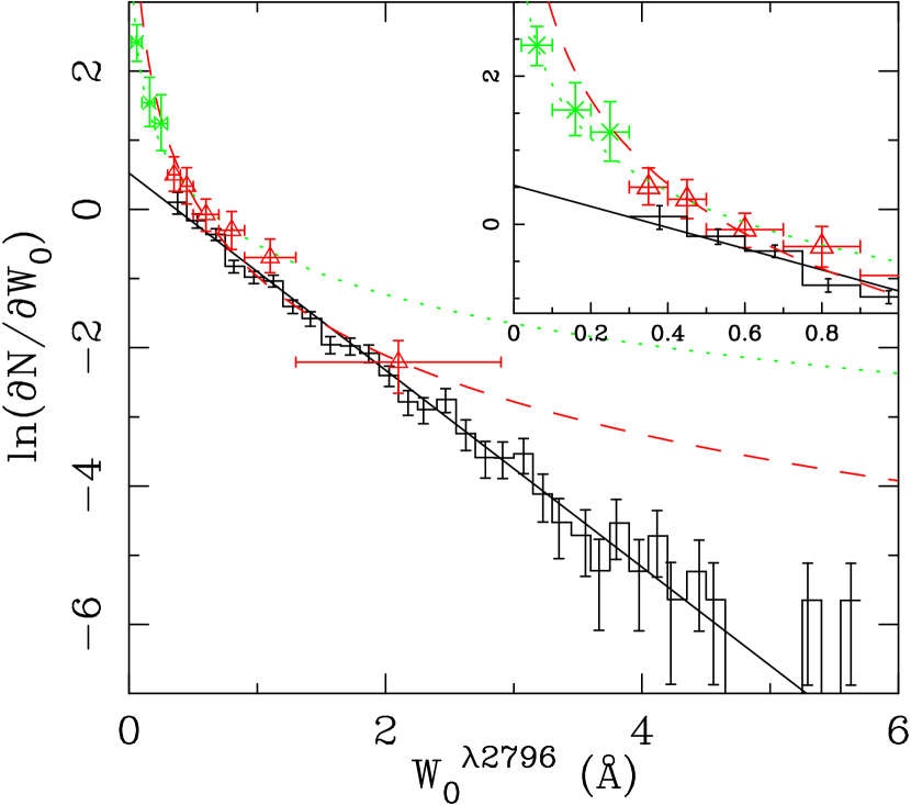
Figure 3: Histogram of the $W_{0}^{\lambda 2796}$ distribution. The solid line is a maximum likelihood fit of the form $\partial N/\partial W_{0}^{\lambda 2796}=\frac{N^{*}}{W^{*}}e^{-\frac{W}{W^{*}}}$ with $W^{*}=0.702\pm 0.017$ Å and $N^{*}=1.187\pm 0.052$. The open triangles are from SS92. The dashed line is their best fit power law. The $\times$ symbols represent data from CRCV99. The dotted line is their power law fit to their binned data plus the SS92 data, excluding the highest-$W_{0}^{\lambda 2796}$ SS92 bin. The inset shows the $W_{0}^{\lambda 2796}<1.0$ Å region in more detail. The power laws greatly over-predict the incidence of strong ($W_{0}^{\lambda 2796}>2$ Å) systems, while our exponential under-predicts the incidence of $W_{0}^{\lambda 2796}<0.3$ Å systems. This suggests a transition in the $\partial N/\partial W_{0}^{\lambda 2796}$ distribution around $W_{0}^{\lambda 2796}\approx 0.3$ Å, possibly indicative of multiple distinct populations.

where $g_{i}(W_{0}^{\lambda 2796},z)=1$ if $W_{0}^{lim}(z)\leq W_{0}^{\lambda 2796}$ and $g_{i}(W_{0}^{\lambda 2796},z)=0$ otherwise, and the redshift limits are defined to be 3,000 km s^-1 above Ly$\alpha$ emission and 3,000 km s^-1 below Mg II emission, or the limits of the data. BAL regions were masked out. The redshift path coverage is shown in Figure 2. Figures 1 and 2 were combined to form an unbiased $W_{0}^{\lambda 2796}$ distribution, which is shown in Figure 3. The distribution is fit very well by an exponential,

$$\partial N/\partial W_{0}^{\lambda 2796}=\frac{N^{*}}{W^{*}}e^{-\frac{W_{0}}{W^{*}}},$$ (4)

with the maximum likelihood value $W^{*}=0.702\pm 0.017$ Å and corresponding $N^{*}=1.187\pm 0.052$. The reduced $\chi^{2}$ comparing the maximum likelihood fit to the binned data is close to unity, independent of the choice of bin size. Also shown are data from CRCV99 with $W_{0}^{\lambda 2796}<0.3$ Å and SS92 with 0.3 Å $\leq W_{0}^{\lambda 2796}\leq 2.9$ Å. All three data sets have similar average absorption redshifts: the CRCV99 data has $\left<z_{abs}\right>=0.9$, and our SDSS EDR and the SS92 data have $\left<z_{abs}\right>=1.1$. The SS92 best-fit exponential closely agrees with our SDSS results, although our normalization, $N^{*}/W^{*}$, is slightly ($\approx 1\sigma$) lower than the SS92 value ($W^{*}=0.66\pm 0.11$ Å, $N^{*}=1.55\pm 0.20$). The reason for this offset, as well as the lack of scatter as compared to the size of the error bars in the SS92 data, is not clear. We note that both our survey and the CRCV99 study consider systems within 500 km s^-1 as a single system, while the SS92 study uses a 1,000 km s^-1 window. This cannot be the source of the normalization offset, however, as it would have the opposite effect, reducing the number of systems found by SS92.

A power law fit of the form $\partial N/\partial W_{0}^{\lambda 2796}=C\,W_{0}^{-\delta}$ with the SS92 values of $C=0.38$ and $\delta=1.65$ is shown as a long-dash line in Figure 3. It is a good fit to our data for 0.5 Å $\lesssim W_{0}^{\lambda 2796}\lesssim 2.0$ Å. For large values of $W_{0}^{\lambda 2796}$, however, the SS92 power law over-predicts $\partial N/\partial W_{0}^{\lambda 2796}$ by almost an order of magnitude. CRCV99 also fit a power law to their binned data combined with the SS92 binned data, but excluding the highest SS92 bin. This is shown as a dotted line. The combined data sets suggest a transition in $\partial N/\partial W_{0}^{\lambda 2796}$ occurring near $\approx$ 0.3 Å.

We used our simulated catalogs (§2.4) to test for biases in the $W_{0}^{\lambda 2796}$ distribution. We chose lines randomly from the input catalog according to a distribution of the form $\partial N/\partial W_{0}^{\lambda 2796}\propto e^{-\frac{W_{0}}{W^{*}_{in}}}$, with an initial guess for $W^{*}_{in}$, until the number of lines recovered were equal to that of the actual catalog, which determines $N^{*}_{in}$. Lines with input $W_{0}^{\lambda 2796}<0.3$ Å were used, although only lines with recovered $W_{0}^{\lambda 2796}\geq 0.3$ Å were retained. We determined a maximum-likelihood value for $W^{*}_{out}$ using the recovered $W_{0}^{\lambda 2796}$ values. We then corrected our guess for $W^{*}_{in}$ to minimize $|W^{*}_{out}-W^{*}_{data}|$. The process was repeated several times with different seeds of the random number generator to determine variance.

Except for the weakest systems in our catalog, which were under-predicted, this simulation was able to match the actual data well. The under-prediction could be a weakness of our simulation, as we had few systems with $W_{0}^{\lambda 2796}<0.3$ Å with which to model the low $W_{0}^{\lambda 2796}$ end of the distribution. Alternatively, the actual distribution could diverge from the simulated exponential for $W_{0}^{\lambda 2796}<0.3$ Å, as suggested by the CRCV99 data. Thus, though we simulated the entire range $W_{0}^{\lambda 2796}\geq 0.3$ Å, we limited the calculation of $W^{*}_{out}$ to $W_{0}^{\lambda 2796}\geq 0.5$ Å. Motivated by the CRCV99 results, we then added a second exponential to the input distribution while holding fixed the primary distribution. We adjusted the values of $W^{*}$ and $N^{*}$ for this second exponential to minimize a $\chi^{2}$ statistic calculated by comparing the binned simulated output to the binned data. Thus, we model the input distribution with separate “weak” and “strong” components:

$$\partial N/\partial W_{0}^{\lambda 2796}=\frac{N^{*}_{wk}}{W^{*}_{wk}}\,e^{-W_{0}/W^{*}_{wk}}+\frac{N^{*}_{str}}{W^{*}_{str}}\,e^{-W_{0}/W^{*}_{str}}.$$ (5)

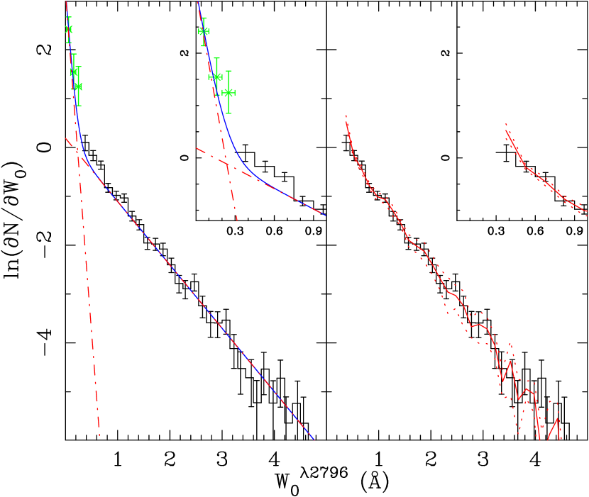
Figure 4: Monte Carlo results. The histograms represent the data. The points are from CRCV99. The left panel shows the input exponential distributions. The shallower exponential ($W^{*}=0.771$ Å and $N^{*}=0.932$) was chosen such that the simulated output distribution had $W^{*}_{out}=W^{*}_{data}$ for $W_{0}^{\lambda 2796}\geq 0.5$ Å. The steeper exponential ($W^{*}=0.072$ Å and $N^{*}=1.71$) was then chosen to minimize the $\chi^{2}$ computed by comparing the total simulated binned data to the real binned data. The solid line is the sum of the two exponential fits. The right panel shows the simulated output (solid line) over-plotted on the data. The dotted lines represent the square root of the variance from different random number seeds.

The resulting best fit values are $N^{*}_{wk}=1.71\pm 0.02$ and $W^{*}_{wk}=0.072\pm 0.001$ Å, and $N^{*}_{str}=0.932\pm 0.011$ and $W^{*}_{str}=0.771\pm 0.014$ Å, where the errors are the square root of the variances from different choices of random number generator seed. These results are shown in Figure 4. The “weak” values were very stable under changes in the seed, producing small variances. Since the “weak” component was constrained by only a small region of $W_{0}^{\lambda 2796}$-space in the data, the actual uncertainties in the parameters are much larger than the variance.

Although most of the systems in our sample are at least partially saturated, the distribution of DR values (see section §3.5) indicates that the typical degree of saturation increases from a mixture at $W_{0}^{\lambda 2796}\lesssim 1$ Å to virtually all systems being highly saturated at $W_{0}^{\lambda 2796}\gtrsim 2$ Å. Thus, we note the possibility that if the column density distribution (which is not measurable with SDSS data) is described by a power law over the range of line strengths in our sample, curve-of-growth effects could conceivably cause the corresponding $\partial N/\partial W_{0}^{\lambda 2796}$ to deviate from a power law at $W_{0}^{\lambda 2796}\gtrsim 2$ Å consistent with our results. Nonetheless, the directly measurable $\partial N/\partial W_{0}^{\lambda 2796}$ is parameterized very well by a single exponential for systems with 0.3 Å $\leq W_{0}^{\lambda 2796}\lesssim 5$ Å, and by two exponentials for $W_{0}^{\lambda 2796}\geq 0.02$ Å.

3.1.1 Redshift Evolution of $N^{*}$ and $W^{*}$

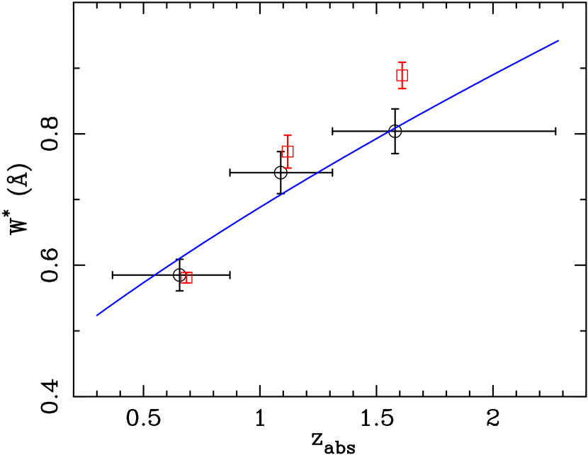
Figure 6: The redshift evolution of $W^{*}$. The horizontal bars represent the bin sizes. The open circles are from the data, while the squares represent the Monte Carlo input values (see text, §3.1). The points are offset slightly in z_abs for clarity. The solid line is the prediction for $W^{*}$ for a fit of the form $W^{*}(z)\propto(1+z)^{\beta}$ described in §3.3.

In order to investigate evolution in $W^{*}$, we split our sample into three redshift bins, $0.366\leq z<0.871$, $0.871\leq z<1.311$, and $1.311\leq z<2.269$, chosen such that there are an equal number of systems in each bin. The three $\partial N/\partial W_{0}^{\lambda 2796}$ distributions are shown in Figure 5. Figure 6 shows the resulting $W^{*}$ for each redshift bin (circles) and the Monte Carlo input values (squares). The bars represent the variance from the different random number seeds only. The curve in Figure 6 is the power law fit described in §3.3.

3.2 Distribution of Absorption Redshifts

Figure 7 shows the absorption redshift distribution for our sample. Absorption redshifts span the range $0.367\leq z\leq 2.269$. The total number of sightlines with sufficient signal to noise ratio to detect lines with $W_{0}^{\lambda 2796}\geq W_{0}^{min}$ for several values of $W_{0}^{min}$ is shown in Figure 8 as a function of redshift. The conspicuous features at $z>1.5$ are due to poor night sky subtractions in many of the spectra. The depression near $z=1.1$ is due to the dichroic (Stoughton et al. 2002.)

The incidence and variance of lines in an interval of $W_{0}^{\lambda 2796}$ over a specified redshift range are given by:

$$\frac{\partial N}{\partial z}=\sum_{i}\frac{1}{\Delta Z\,(W_{0}^{i})},\ \ \ \sigma^{2}_{\frac{\partial N}{\partial z}}=\sum_{i}\,\left(\frac{1}{\Delta Z\,(W_{0}^{i})}\right)^{2},$$ (6)

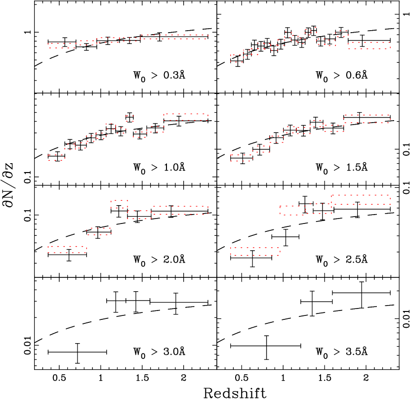
Figure 9: Number density evolution of Mg II absorbers for $W_{0}^{\lambda 2796}\geq W_{0}^{min}$ samples. The dashed lines are the no-evolution curves for a WMAP cosmology, ($\Omega_{M},\Omega_{\Lambda},h_{0})=(0.3,0.7,0.7)$. The curves are normalized to minimize the $\chi^{2}$ to the binned data. The $W_{0}^{min}=$ 0.3 Å, 0.6 Å, 1.0 Å, and 1.5 Å samples have $\chi^{2}$ values that are consistent with no evolution. The $W_{0}^{min}=$ 2.0 Å, 2.5 Å, and 3.0 Å samples are inconsistent with the no evolution curves at $\gtrsim 3\sigma$, while the $W_{0}^{min}=$ 3.5 Å sample is inconsistent at $\simeq 2\sigma$. The dotted boxes represent the results of the Monte Carlo simulation. The widths correspond to the bin sizes and the heights to the $\pm 1\sigma$ values. The $W_{0}^{min}=$ 3.0 Å and 3.5 Å samples were not large enough to permit meaningful Monte Carlo simulations.

where the sum is over systems with $W_{0}^{i}$ in the given interval and $\Delta Z\,(W_{0}^{i})$ represents the path contained in the specified redshift range. Traditionally, $\partial N/\partial z$ has been plotted versus redshift for lines stronger than a specified $W_{0}^{min}$. In Figure 9, we show $\partial N/\partial z$ as a function of redshift for $W_{0}^{\lambda 2796}\geq$ 0.3 Å, 0.6 Å, 1.0 Å, 1.5 Å, 2.0 Å, 2.5 Å, 3.0 Å and 3.5 Å. Also shown in Figure 9 are the no-evolution curves (NECs) for a cosmology with WMAP results (Spergel et al. 2003), ($\Omega_{M},\Omega_{\Lambda},h)=(0.3,0.7,0.7)$, scaled to minimize the $\chi^{2}$ to the binned data. The $W_{0}^{min}=$ 0.3 Å, 0.6 Å, 1.0 Å, and 1.5 Å samples have $\chi^{2}$ values that are consistent with no evolution. The $W_{0}^{min}=$ 2.0 Å, 2.5 Å, and 3.0 Å samples are inconsistent with the NECs at $\gtrsim 3\sigma$, while the $W_{0}^{min}=$ 3.5 Å sample is inconsistent at $\approx 2\sigma$. The dotted-boxes in Figure 9 show the results of the Monte Carlo simulation described in §2.4.

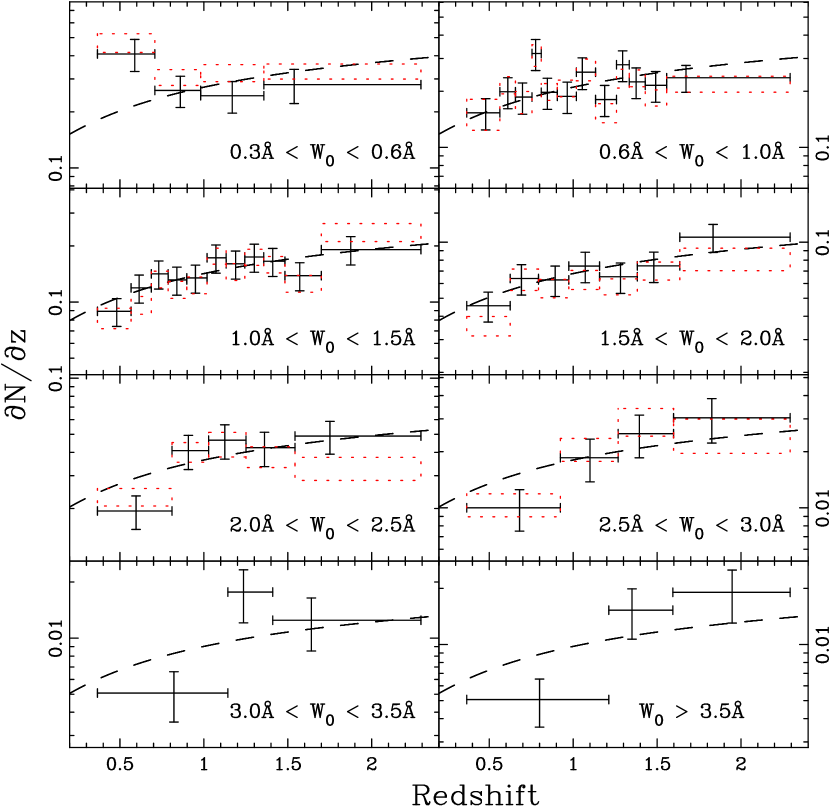
Figure 10: Number density evolution of Mg II absorbers for ranges of $W_{0}^{\lambda 2796}$. The dashed lines are the no-evolution curves for a WMAP cosmology, ($\Omega_{M},\Omega_{\Lambda},h_{0})=(0.3,0.7,0.7)$. The curves are normalized to minimize the $\chi^{2}$ to the binned data. The 0.6 Å - 1.0 Å, 1.0 Å - 1.5 Å, 1.5 Å - 2.0 Å, 2.0 Å - 2.5 Å and 2.5 Å - 3.0 Å samples have $\chi^{2}$ values that are consistent with no evolution. The no-evolution curve for the 0.3 Å - 0.6 Å sample is ruled out at $\simeq 2.5\sigma$ and for the 3.0 Å - 3.5 Å and $\geq 3.5$ Å samples at $\simeq 2.0\sigma$. The dotted boxes represent the results of the Monte Carlo simulation. The widths correspond to the bin sizes and the heights to the $\pm 1\sigma$ values. The 3.0 Å - 3.5 Å and greater than 3.5 Å samples were not large enough to permit meaningful Monte Carlo simulations.

The large size of our data set allows us to investigate $\partial N/\partial z$ not only for distributions cumulative in $W_{0}^{\lambda 2796}$, but also for ranges of $W_{0}^{\lambda 2796}$. This is potentially important, as evolution in the largest $W_{0}^{\lambda 2796}$ values is not necessarily negligible in cumulative $\partial N/\partial z$ distributions. Thus, we repeated the above analysis for the following ranges: 0.3 Å $\leq W_{0}^{\lambda 2796}<$ 0.6 Å, 0.6 Å $\leq W_{0}^{\lambda 2796}<$ 1.0 Å, 1.0 Å $\leq W_{0}^{\lambda 2796}<$ 1.5 Å, 1.5 Å $\leq W_{0}^{\lambda 2796}<$ 2.0 Å, 2.0 Å $\leq W_{0}^{\lambda 2796}<$ 2.5 Å, 2.5 Å $\leq W_{0}^{\lambda 2796}<$ 3.0 Å, 3.0 Å $\leq W_{0}^{\lambda 2796}<$ 3.5 Å, and $W_{0}^{\lambda 2796}\geq$ 3.5 Å. The results are shown in Figure 10. The 0.6 Å - 1.0 Å, 1.0 Å - 1.5 Å, 1.5 Å - 2.0 Å, 2.0 Å - 2.5 Å and 2.5 Å - 3.0 Å samples have $\chi^{2}$ values that are consistent with no evolution. The NEC for the 0.3 Å - 0.6 Å sample is ruled out at $\approx 2.5\sigma$ and for the 3.0 Å - 3.5 Å and $\geq$ 3.5 Å samples at $\approx 2.0\sigma$.

Since the NEC normalization is a free parameter, a plot cumulative in redshift comparing $\partial N/\partial z$ from the data to the NEC is more instructive. These plots, shown in Figures 11 and 12, highlight the skew of the $\partial N/\partial z$ curves from the NEC prediction that is not necessarily manifested in the $\chi^{2}$ analysis. The NECs over-predict $\partial N/\partial z$ at low redshift for small $W_{0}^{min}$ and under-predict $\partial N/\partial z$ at low redshift for large $W_{0}^{min}$. The transition occurs for the cumulative $W_{0}^{\lambda 2796}$ plots between $W_{0}^{min}=$ 0.6 Å and 1.0 Å  and the effect is stronger for increasingly larger values of $W_{0}^{min}$. The plots using ranges of $W_{0}^{\lambda 2796}$ show that the transition from over- to under- predicting $\partial N/\partial z$ at lower redshift occurs around 1 Å, and significant detection of evolution is seen in systems with $W_{0}^{\lambda 2796}\gtrsim$ 2.0 Å. The evolution signal is strong ($\approx 4\sigma$) for lines with $W_{0}^{\lambda 2796}\geq$ 3.5 Å. Although these plots do give a clearer indication of the deviation from the NECs, it is difficult to ascribe a K-S probability to the curves in Figures 11 and 12 because systems contribute to $\partial N/\partial z$ in a non-uniform manner, i.e., inversely proportional to $g(W_{0},z)$.

The $\partial N/\partial z$ point in the lowest redshift bin for the $W_{0}^{\lambda 2796}\geq$ 0.3 Å  sample in Figure 9, and for the 0.3 Å $\leq W_{0}^{\lambda 2796}<$ 0.6 Å sample in Figure 10, lie well above the NEC. The increase is greater in magnitude but smaller in significance ($\approx 2\sigma$ versus $\approx 3\sigma$) for the non-cumulative sample. The Monte Carlo results lessen the significance in the cumulative sample, but not in the non-cumulative sample. Thus, the weakest lines in our study show evolution in the sense that their incidence increases with decreasing redshift. However, this may be an artifact of the sharp cutoff in our sample at 0.3 Å. A sample with $W_{0}^{\lambda 2796}\geq$ 0.4 Å is consistent with the NEC, and $\partial N/\partial z$ for 0.4 Å $\leq W_{0}^{\lambda 2796}<$ 0.6 Å is within $1\sigma$ of the NEC at all redshifts. We cannot exclude the possibility, however, that the increase is real.

A comparison of the $\partial N/\partial z$ values from our survey and SS92 for the full redshift ranges are shown in Table 1. Our $W_{0}^{\lambda 2796}\geq$ 0.6 Å and 1.0 Å results are consistent with SS92. However, we find a smaller value of $\partial N/\partial z$ for $W_{0}^{\lambda 2796}\geq$ 0.3 Å (although this difference is confined to $z\gtrsim 1.3$.)

3.3 Joint $W_{0}^{\lambda 2796}$-Redshift Distribution

Conventionally, the $W_{0}$-redshift distribution of absorption lines, $\partial^{2}N/\partial z\,\partial W_{0}$, has been parameterized by a combination of a power law in redshift and exponential in $W_{0}$ (e.g., Murdoch et al. 1986; Lanzetta, Turnshek & Wolfe 1987; Weymann et al. 1998):

$$dN/dW_{0}=\frac{N^{*}}{W^{*}}e^{-\frac{W_{0}}{W^{*}}},\ \ dN/dz=N_{0}\,(1+z)^{\gamma}.$$ (7)

This parameterization is convenient for the determination of best-fit values for the parameters because of the separate $W_{0}$ and $z$ dependences. However, our data reveal that a single power law is not a good fit to $\partial N/\partial z$ for any given range of $W_{0}^{\lambda 2796}$. Also, we have shown that $W^{*}$ depends on redshift for Mg II $\lambda 2796$ lines (i.e., $\partial N/\partial z$ for different ranges of $W_{0}^{\lambda 2796}$ varies differently with redshift.) We do not wish to abandon the exponential form, however, as we have also shown that it is a very good parameterization of the data at all redshifts for the range of $W_{0}^{\lambda 2796}$ covered by our sample. Thus, we retain the general form $\partial N/\partial W_{0}^{\lambda 2796}=\frac{N^{*}}{W^{*}}\,e^{-\frac{W_{0}}{W^{*}}}$, but allow both $N^{*}$ and $W^{*}$ to vary with redshift as a power law in $(1+z)$. The maximum likelihood results are $N^{*}=1.001\pm 0.132\,(1+z)^{0.226\pm 0.170}$ and $W^{*}=0.443\pm 0.032\,(1+z)^{0.634\pm 0.097}$ Å. The values are highly correlated, and the errors include the effects of the correlations. See the Appendix for details of our parameterization and a discussion of the errors.

We repeated the analyses of §3.2, comparing the $\partial N/\partial z$ curves to those determined using our redshift parameterization of $N^{*}$ and $W^{*}$. The results, shown in Figures 13 and 14, indicate that our parameterization is indeed a good description of all of the data. The evolution is well described by a steepening of the $W_{0}^{\lambda 2796}$ distribution with a normalization that changes so as to keep $\partial N/\partial z$ constant for the smaller $W_{0}^{\lambda 2796}$ values. Extrapolating our parameterization to lower redshift, we predict $\partial N/\partial z=0.28\pm 0.03$ for $W_{0}^{\lambda 2796}\geq 0.6$ Å and $\left<z\right>=0.06$ and $\partial N/\partial z=0.11\pm 0.02$ for $W_{0}^{\lambda 2796}\geq 1.0$ Å and $\left<z\right>=0.04$, in comparison to Churchill’s (2001) values of $\partial N/\partial z=0.22^{+0.12}_{-0.09}$ and $\partial N/\partial z=0.16^{+0.09}_{-0.05}$, respectively. However, our parameterization is likely inappropriate for describing $W_{0}^{\lambda 2796}<0.3$ Å lines, since not including the apparently two-component nature of the $W_{0}^{\lambda 2796}$ distribution leads to underestimates of the number density of weak lines (Figure 3).

Table 2 summarizes the various parameterizations of the data.

3.4 Systematic Errors

Our Monte Carlo simulations did not uncover any significant systematic errors. All of the Monte Carlo $\partial N/\partial z$ values are consistent with those from the data. However, since we used the data to model the simulated lines, if there are lines with characteristics that make them underrepresented in the data, they would also be underrepresented in the simulated catalogs. We ran simulations to address this issue as we developed our line-finding algorithm. Although it is possible that we miss certain types of lines, such as weak kinematic outliers or lines with abnormally broad or exotic profiles, for example, these effects are likely to be small.

A potentially more serious source of systematic error may arise in the regions of poorly subtracted night sky lines seen in some of the spectra. The error arrays are not always accurate in these regions, and doublets falling between sky lines can be confused with residuals from the poor subtraction. As the errors are larger (though not necessarily accurate) in the night sky regions, the values of $W_{0}^{lim}$ are large as well. Thus, only the strongest lines would be affected. In principle, our simulations should account for these effects. However, since non-Gaussian profiles are preferentially found among the stronger lines, their simulation is somewhat less reliable. Also, their numbers are much smaller, providing fewer lines to serve as models in the simulation, and less overall significance. The largest $W_{0}^{\lambda 2796}$ ranges were, in fact, too sparse for meaningful simulations. Errors of this type would be manifest in the largest $W_{0}^{\lambda 2796}$ ranges and for redshifts $z\sim 1.6-2.0$.

Finally, in QSO absorption-line studies it is of interest to asses if biases due to the presence of the absorber affecting the magnitude and color of the background QSO are present. The most often discussed effect is that of a dimming and reddening of the background QSO due to dust in the absorber. However, the presence of an absorbing galaxy could also contribute light and/or have a lensing effect, causing the QSO to appear brighter. These competing effects are investigated, using the absorbers and simulations from this work, in Ménard, Nestor, & Turnshek (2004). They find that QSOs with Mg II absorbers tend to be brighter in red passbands and fainter in blue passbands, indicating a combination of brightening and reddening. The effects are stronger for increasingly stronger $W_{0}^{\lambda 2796}$ systems. The average effects are mostly within $\pm 0.2$ magnitudes. As the SDSS EDR QSO catalog selection properties were not necessarily homogeneous, it is difficult to quantify the effect these results may have on our data. If these effects are non-negligible, they could affect the measured $W_{0}^{\lambda 2796}$ distribution and $\partial N/\partial z$. The biases are likely to be small, however, since it would be peculiar if they conspired to drive $\partial N/\partial W_{0}^{\lambda 2796}$ to more closely resemble an exponential, and there is no detectable deviation from an exponential, consistent with the expected biases, seen in Figure 3. Since dust increases with decreasing redshift (consistent with the findings of Nestor et al. 2003), it is worth considering if the evolution in $\partial N/\partial z$ seen for the strongest systems is an affect of increasing dust. However, Ménard et al. find no such increase in bias with decreasing redshift. Also, Ellison et al. (2004) compare Mg II $\partial N/\partial z$ determined from radio-selected CORALS survey spectra to values obtained with optical surveys (including this work), and find good agreement (though they do not investigate the largest $W_{0}^{\lambda 2796}$ ranges). Therefore, the steepening of the $W_{0}^{\lambda 2796}$ distribution due to a disappearance of the largest $W_{0}^{\lambda 2796}$ lines at low redshift and the evolution in $\partial N/\partial z$ for strong lines appears to be real.

While more recent SDSS QSO spectra offer the opportunity to increase the Mg II absorber sample by another order of magnitude, systematic errors in line identification and measurement will begin to dominate in the determination of absorber property statistics.

3.5 Mg II Doublet Ratio

Mg II doublet ratios span the range from $DR=2.0$ for completely unsaturated systems to $DR=1.0$ for completely saturated systems. Figure 15 shows the $DR$ distribution for our sample. The doublets are, for the most part, saturated. Ninety percent of doublets with a measured $DR$ are within $3\sigma$ of $DR=2.0$, and 92% have $DR-1.0>\sigma_{DR}$. Figure 16 shows $DR$ as a function of redshift. There is no detectable evolution in the $DR$ distribution. In fact, the $DR$ distribution is remarkably consistent over the three redshift ranges of Figures 5 and 6.

3.6 Mg II Velocity Dispersions

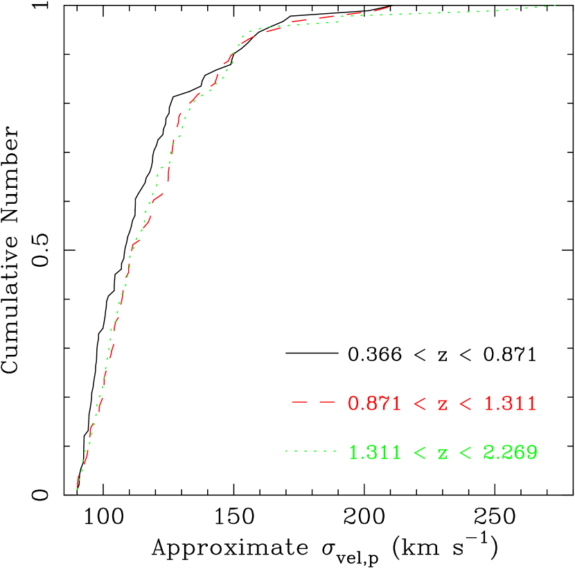
Figure 17: Cumulative distribution of approximate velocity dispersions for $\sigma_{vel,p}>90$ km s^-1. The lower and middle redshift bins differ in K-S probability at the $\approx 1\sigma$ level.

For absorption lines that are at least partially saturated, such as those that dominate our sample, $W_{0}^{\lambda 2796}$ is primarily a measure of the number of kinematic subcomponents along the line of sight (Petitjean & Bergeron 1990) and, to a lesser extent, projected velocity dispersion, $\sigma_{vel,p}$ (see, for example, Churchill et al. 2000, hereafter C2000). We can directly extract information about $\sigma_{vel,p}$ for individual systems by deconvolving the fitted profile from the line spread function. However, as most of the $\lambda 2796$ lines are only mildly resolved, this approach is not sensitive for all but the most resolved systems. Nonetheless, we investigated the evolution of the $\sigma_{vel,p}$ distribution over the three redshift ranges of Figures 5 and 6. In all three redshift ranges, $\simeq 80\%$ of the systems have measured values of $\sigma_{vel,p}<90$ km s^-1. Comparing just systems with $\sigma_{vel,p}>90$ km s^-1, we find that $\sigma_{vel,p}$ tends to be smaller in the lowest redshift bin (see Figure 17). However, the middle- and lower-redshift bin velocity distributions only differ at the $1\sigma$ level.

3.7 Fe II $\lambda 2600$ and Mg I $\lambda 2852$

Figure 18 shows the distribution of Fe II $W_{0}^{\lambda 2600}$ for our sample. The error-weighted mean is $\left<W_{0}^{\lambda 2796}/W_{0}^{\lambda 2600}\right>=1.42$ and the distribution has a smooth tail extending out to large values, though ratios above $\approx 4$ are dominated by values with significance less than $3\sigma$. Figure 19 shows the distribution of Mg I $W_{0}^{\lambda 2852}$ for our sample. The error-weighted mean is $\left<W_{0}^{\lambda 2796}/W_{0}^{\lambda 2852}\right>=4.14$ and the distribution has a smooth tail extending out to large values, though ratios above $\approx 8$ are dominated by values with significance less than $3\sigma$.

4 Discussion

The determination of $\partial^{2}N/\partial z\,\partial W_{0}^{\lambda 2796}$ provides insight into the nature of the systems comprising the population of Mg II absorbers. Specifically, the inability of a single functional form to describe $\partial N/\partial W_{0}^{\lambda 2796}$ suggests that multiple physical populations contribute to the absorption. Additionally, $\partial N/\partial W_{0}^{\lambda 2796}$ can be used to infer average absorption cross sections for a given $W_{0}^{\lambda 2796}$ regime. The $W_{0}^{\lambda 2796}$-dependent evolution of $\partial N/\partial z$ holds further clues related to the nature of Mg II absorbers. These issues are discussed below. We also note that a significant fraction ($\approx$ 36%) of Mg II systems with $W_{0}^{\lambda 2796}\geq 0.5$ Å and $W_{0}^{\lambda 2600}\geq 0.5$ Å are DLAs. The implications of the evolution in the Mg II $\partial N/\partial z$ to $\Omega_{DLA}$ will be discussed in Rao, Turnshek, & Nestor (2004).

4.1 The Nature of the Absorbers

The distribution of $W_{0}^{\lambda 2796}$ for absorbers with $W_{0}^{\lambda 2796}\geq 0.3$ Å is fit very well by a single exponential. However, extrapolating this exponential to smaller values of $W_{0}^{\lambda 2796}$ under-predicts the incidence of lines (Figure 3), motivating a two-component description of the form of Equation 5. This is the first clear indication of such a transition and raises the question of whether the ensemble of clouds comprising Mg II absorbers are the result of two physically distinct populations.

In a series of papers using HIRES/Keck data (Charlton & Churchill 1998; C2000; Churchill & Vogt 2001; Churchill, Vogt, & Charlton 2003), Churchill and collaborators have investigated the kinematic structure of Mg II absorbers at $0.4<z\lesssim 1.2$. For intermediate/strong absorbers ($W_{0}^{\lambda 2796}\geq 0.3$ Å), they show that the absorption systems are composed of multiple kinematic subsystems, usually containing a dominant subsystem (ensemble of clouds) with a velocity width $\approx 10-15$ km s^-1 and a corresponding H I column density which is optically thick at the Lyman limit (i.e., $N_{H\,I}\gtrsim 3\times 10^{17}$ atoms cm^-2). Additionally, a number of weaker, often unresolved (at $\approx$6 km s^-1 resolution) subsystems (clouds) with a large spread of velocity separations (up to $\approx 400$ km s^-1) from the systemic velocity of the absorber are usually present (see Churchill & Vogt 2001, Figure 7.) These weaker subsystems typically contribute only 10%-20% of the rest equivalent width. The strongest Mg II absorbers ($W_{0}^{\lambda 2796}\gtrsim 2$ Å) often contain more than one of the dominant subsystems and have equivalent widths dominated by saturated features.

CRCV99 presented a HIRES/Keck study of weak ($W_{0}^{\lambda 2796}<0.3$ Å) Mg II absorption systems. The properties of the kinematic subsystems comprising weak Mg II absorbers are similar to the weak subsystems of intermediate/strong Mg II absorbers. The individual clouds have $W_{0}^{\lambda 2796}\lesssim 0.15$ Å and sub-Lyman limit H I columns.

Although most of the Mg II $\lambda 2796$ lines in our survey are at least partially saturated, the degree of saturation is correlated with $W_{0}^{\lambda 2796}$. For example, the DR values for systems with 0.3 Å $\lesssim W_{0}^{\lambda 2796}\lesssim 1$ Å indicate a mix in degree of saturation. For lines in this regime, $\partial N/\partial W_{0}^{\lambda 2796}$ is sensitive to the distribution of Mg II column densities, $\partial N/\partial N_{Mg\,II}$. In fact, Churchill & Vogt (2001) and Churchill, Vogt, & Charlton (2003) find almost identical power law slopes for $\partial N/\partial W_{0}^{\lambda 2796}$ and $\partial N/\partial N_{Mg\,II}$ in their 0.3 Å $\leq W_{0}^{\lambda 2796}\leq 1.5$ Å sample. Systems with $W_{0}^{\lambda 2796}\gtrsim 2$ Å, however, are almost always highly saturated. Also, a general distinction between weak ($W_{0}^{\lambda 2796}<0.3$ Å) and intermediate/strong ($W_{0}^{\lambda 2796}\geq 0.3$ Å) Mg II absorbers is the absence or presence of a “dominant” subsystem, though the differences are neither discrete nor without exception. Additionally, Rigby, Charlton, & Churchill (2002) note a substantial excess of Mg II absorbers that are comprised of a single kinematic component, which are almost exclusively weak absorbers. Therefore, given the form of $\partial N/\partial W_{0}^{\lambda 2796}$, it is appropriate to consider a picture in which the sum of the weaker kinematic subsystems (clouds) in an absorber are described by $N^{*}_{wk}$ and $W^{*}_{wk}$, and the stronger (dominant ensembles) subsystems by $N^{*}_{str}$ and $W^{*}_{str}$. If this multi-population explanation is indeed correct, the nature of these populations needs to be explained. First, we consider the weak subsystems.

It has been demonstrated that absorption line systems can be associated with galaxies out to large galactocentric distances ($\approx 100h^{-1}$ kpc for C IV and $\approx 200h^{-1}$ kpc for Ly$\alpha$ absorbers, for example; Chen, Lanzetta, & Webb 2001; Chen et al. 2001). Though there is evidence for Ly$\alpha$ absorbers in voids (Penton, Stocke, & Shull 2002), these appear to be limited to the weakest systems. Also, Rigby, Charlton, & Churchill (2002) conclude that a significant fraction of relatively strong ($10^{15.8}$ cm${}^{-2}\lesssim$ $N_{H\,I}\lesssim 10^{16.8}$ cm^-2) Ly$\alpha$ forest lines are associated with single-cloud weak Mg II absorbers, which are also C IV absorbers.

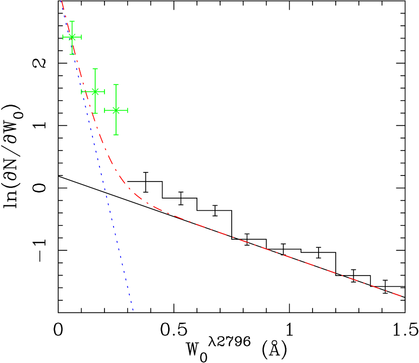
Figure 20: Predicted $\partial N/\partial W_{0}^{\lambda 2796}$ for Ly$\alpha$ forest/single-cloud Mg II . The solid line is the maximum likelihood fit to our data with $W_{0}^{\lambda 2796}\geq 0.5$ Å. The dotted line is the approximation for single-cloud Mg II $\partial N/\partial W_{0}^{\lambda 2796}$ using data from CRCV99 and a normalization from Rigby, Charlton, & Churchill (2002). The dot-dash curve is the sum of the two distributions. The points are from CRCV99.

Therefore, we consider whether single-cloud/Ly$\alpha$ forest absorbers at relatively large galactocentric distances can contribute significantly to our “weak” component of $\partial N/\partial W_{0}^{\lambda 2796}$. CRCV99 claim to be 91% complete down to $W_{0}^{\lambda 2796}=0.03$ Å. Thus, using the measurements of single-cloud systems from CRCV99 with $W_{0}^{\lambda 2796}\geq 0.03$ Å, we find $W^{*}_{sc}=0.063\pm 0.015$ Å. Rigby, Charlton, & Churchill (2002) give a $\partial N/\partial z$ value for the single-cloud systems, which can be used to normalize $\partial N_{sc}/\partial W_{0}^{\lambda 2796}$. While our comparison is approximate in that the redshift range covered by the C2000 sample, $0.4<z<1.4$, is different than that of our sample, the result shown in Figure 20 demonstrates that the single-cloud/Ly$\alpha$ forest systems should contribute significantly to the upturn in $\partial N/\partial W_{0}^{\lambda 2796}$, especially for the weakest systems.

Although the Mg II absorber galaxy population has been shown to span a range of galaxy colors and types, Steidel, Dickinson, & Persson (1994) describe the “average” galaxy associated with an intermediate/strong Mg II absorber galaxy as one which is consistent with a typical $0.7L^{*}$ Sb galaxy. Furthermore, Steidel at al. (2002, also see Ellison, Mallén-Ornelas, & Sawicki 2003) compare the galaxy rotation curves to the absorption kinematics for a sample of high inclination spiral Mg II absorption galaxies. They find extended-disk rotation dominant for the absorption kinematics, though a simple disk is unable to explain the range of velocities, consistent with a disk plus halo-cloud picture. However, there are several counter evidences to a rotating disk description for the dominant subsystems. The most important is that imaging often fails to reveal a disk galaxy in proximity to the absorption line of sight. DLA galaxies, which are a subset of strong Mg II absorbing galaxies, are not dominated by classic spirals. Of the 14 identified DLA galaxies summarized in Rao et al. (2003), only six are spirals. Furthermore, systems that have been studied without the discovery of the absorbing galaxy despite deep imaging rule out at least bright spirals (although disky-LSBs may still contribute.) Bright galaxies near QSO sightlines usually show Mg II absorption, but not all strong Mg II absorbers have a nearby spiral or bright galaxy. Thus, though it is clear that rotating disks do contribute to the population comprising the dominant kinematic subsystem(s) of $W_{0}^{\lambda 2796}\geq 0.3$ Å absorbers, they can only account for a (perhaps small) fraction of the total population.

The detailed nature of the remaining contribution is yet unclear, but this dichotomy supports the idea of multiple populations. Bond et al. (2001), for example, show that the kinematics of many strong (defined as $W_{0}^{\lambda 2796}\geq 1.8$ Å in their sample) Mg II absorbers have kinematic structure that is highly suggestive of superwinds/superbubbles. They also show that DLAs exhibit low-ion kinematic profiles distinct from the superwind-like absorbers, which tend to be sub-DLA. Furthermore, imaging studies (e.g., Le Brun et al. 1997; Rao et al. 2003) have found LSB, dwarf, and groups/interacting systems, in addition to some spirals, responsible for strong Mg II absorption systems (though the samples are typically selected to be DLA sightlines). Sightlines through groups and interacting systems are likely to sample large velocity spreads. Apparently, their contribution to the total cross section of strong Mg II systems is non-negligible.

Thus, though a two-component description is sufficient to describe $\partial N/\partial W_{0}^{\lambda 2796}$ within the current data, it is likely that more than two physically distinct populations contribute significantly to the phases comprising the absorbing clouds. By observing a large number of galaxy types that sample a range of $W_{0}^{\lambda 2796}$ and impact parameter, it would be possible to ascertain what populations contribute most directly to the absorber population.

4.2 The Absorber Cross-Sections

The relative mean absorber cross-section, $\sigma(z)$, for ranges of $W_{0}^{\lambda 2796}$ can be determined directly from $\partial N/\partial W_{0}^{\lambda 2796}$. Additionally, knowledge of $\partial N/\partial z$ and the galaxy luminosity function (LF) allows the approximation of the normalization of the mean absorber cross-section, under the assumption that the absorbers arise in galaxies, since $\partial N/\partial z$ is the product of $\sigma(z)$ and the number density of absorbers, $n(z)$. However, the process is inherently uncertain since: (a) the redshift dependence of the galaxy LF is not well determined; (b) although a scaling relation $\sigma(L)\propto(L/L^{*})^{\beta}$ has traditionally been assumed, the determination of $\beta$ is uncertain and likely not universal for all morphological types or redshifts, if it is even appropriate; and (c) depending on the value of $\beta$ and the LF faint-end slope, the minimum absorber galaxy luminosity (which also is likely to be dependent on morphology and redshift) can have large effects in the statistically-determined cross sections.

Nonetheless, an approximate normalization is of physical interest. Thus, we define $R_{eff}$ to be the effective projected radius for absorption such that $\sigma(L)\equiv\pi\,R_{eff}^{2}(L)$. Note that the galactocentric radius within which the absorption may occur (i.e., the range of impact parameter) may be very different than $R_{eff}$. Steidel, Dickinson, & Persson (1994) find absorbing galaxies as faint as $L\sim 0.05\,L^{*}$, and a scaling law for the gaseous cross-section $R_{eff}(L)/R_{eff}^{*}=(L/L^{*})^{0.2}$ for both optical (B-band) and near-IR (K-band) luminosity. They claim the relation is much tighter for the near-IR. Thus, we use the redshift parameterization of the K-band LF from the MUNICS data set (Drory et al. 2003) and $L_{min}=0.05\,L^{*}$, though we also test $L_{min}=0.25\,L^{*}$ and $L_{min}=0.001\,L^{*}$ to investigate the effects of using high/low values of $L_{min}$. We adopt the Dickinson & Steidel (1996) revised scaling law for Mg II systems with $W_{0}^{\lambda 2796}\geq 0.3$ Å, namely $R_{eff}(L_{K})/R_{eff}^{*}=(L_{K}/L_{K}^{*})^{0.15}$.

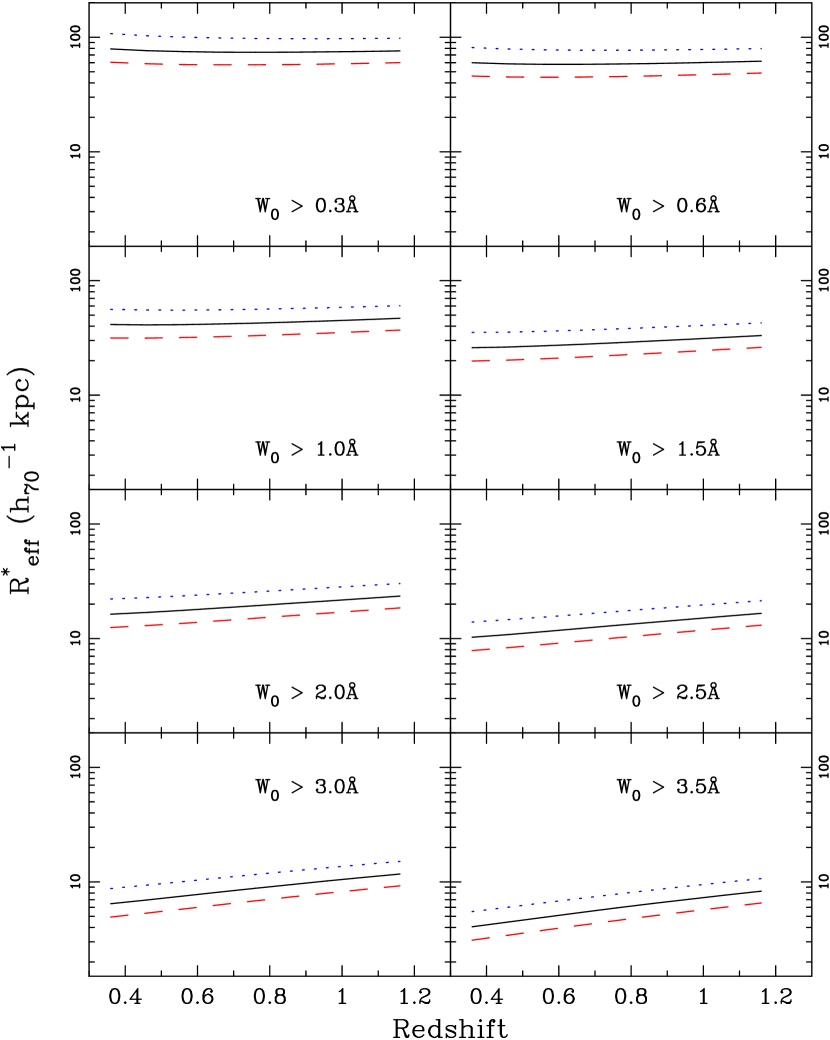
Figure 21: Cross-section estimates $\sigma(L^{*})=\pi\,R_{eff}^{*\,2}$. The solid lines represent the $L_{min}=0.05\,L^{*}$ result. The dashed-lines are for a small value of $L_{min}=0.001\,L^{*}$ and the dotted-lines a large value $L_{min}=0.25\,L^{*}$. We use the redshift parameterization of the K-band LF from the MUNICS data set, a scaling relation $R_{eff}/R_{eff}^{*}=(L/L^{*})^{0.15}$, and $\partial N/\partial z$ from our parameterization (§3.3).

The results for the different $W_{0}^{min}$ values from §3.2 are shown in Figure 21. Despite the limitations of this approach, approximate values for $R^{*}_{eff}$ are apparent: $\approx 60-100\,h_{70}^{-1}$ kpc for $W_{0}^{\lambda 2796}\geq 0.3$ Å, $\approx 30-60\,h_{70}^{-1}$ kpc for $W_{0}^{\lambda 2796}\geq 1.0$ Å, $\approx 15-30\,h_{70}^{-1}$ kpc for $W_{0}^{\lambda 2796}\geq 2.0$ Å and $\lesssim 10\,h_{70}^{-1}$ kpc for $W_{0}^{\lambda 2796}\geq 3.5$ Å. Guillemin & Bergeron (1997) find $R^{*}_{eff}=65\,h_{70}^{-1}$ kpc using the upper envelope of the distribution of observed impact parameters for a sample with 0.3 Å $\leq W_{0}^{\lambda 2796}\leq 4.7$ Å  and $\left<W_{0}^{\lambda 2796}\right>=1.3$ Å. CRCV99 find $R^{*}_{eff}=110\,h_{70}^{-1}$ kpc for their $W_{0}^{\lambda 2796}\geq 0.02$ Å sample, but use a LF normalization that is $\sim 3.5$ times our adopted values. Chen, Lanzetta, & Webb (2001) find $R^{*}_{eff}=137\,h_{70}^{-1}$ kpc for C IV absorbers, which may sample larger galactocentric radii. The $R^{*}_{eff}$ values are averages; it is expected that there are large galaxy to galaxy variations. Direct comparison of $R^{*}_{eff}$ to the distribution of impact parameters would require knowledge of the gas geometry and the (likely $W_{0}^{\lambda 2796}$-dependent) covering factor. For example, small regions that allow large $W_{0}^{\lambda 2796}$ absorption may be found at galactocentric radii $r\gg R_{eff}$ if the covering factor for such absorption is $f\ll 1$.

We also note that for the single-cloud Mg II systems (see §4.1), Rigby, Charlton, & Churchill (2002) derive $\partial N/\partial z=1.1\pm 0.06$. They claim that these systems are 25%-100% of the Ly$\alpha$ forest with $10^{15.8}$ cm${}^{-2}<$ $N$(H I) $<10^{16.8}$ cm^-2. Under the assumption that they can be associated with galaxies, their incidence corresponds to $R^{*}_{eff}\approx 80-120\,h_{70}^{-1}$ kpc in the above approximation. This can be compared to the claim of Chen et al. (2001) that all $N$(H I) $\gtrsim 10^{14}$ cm^-2 Ly$\alpha$ forest lines arise within the characteristic radius $R^{*}\approx 250\,h_{70}^{-1}$ kpc of luminous galaxies.

4.3 Nature of the Evolution

4.3.1 $W_{0}^{\lambda 2796}<0.3$ Å Systems

The Ly$\alpha$ forest $\partial N/\partial z$ is known to decrease strongly over the redshift interval $4\gtrsim z\gtrsim 1.6$, but little evolution is present at lower redshifts (see Weymann 1998, and references therein). In §4.1, we speculated that a portion of the enriched Ly$\alpha$ forest contributes to the weak subsystems found in Mg II absorbers. If this is indeed the case, then this evolution may manifest itself in $\partial N/\partial z$ for the weakest ($W_{0}^{\lambda 2796}<0.3$ Å) Mg II systems at high $z$.

4.3.2 The Lack of Measured Evolution in Intermediate/Strong (0.3 Å $\leq W_{0}^{\lambda 2796}\lesssim 2$ Å) Systems

Our sample covers the redshift interval $z=2.267$ to $z=0.366$ which corresponds to 6.6 Gyrs, or about half the age of the universe. As long assumed and recently demonstrated with the Hubble deep fields (see Ferguson, Dickinson, & Williams 2000 for a review), galaxies were quite different at $z=2.3$ than at $z=0.4$. It is therefore noteworthy that, even with the large absorber sample presented here, relatively little evolution is detected in the bulk of Mg II absorption systems. For example, it is believed that the global star formation rate peaked near $z=1$ and has declined by a factor of $\approx 2$ by $z=0.5$ and by a factor of $\approx 10$ by $z=0$ (Hopkins 2004 and references therein.) Contrastingly, the total cross-section for absorption $n(z)\,\sigma(z)$ of our $W_{0}^{min}=0.6$ Å and 1.0 Å samples evolves $\lesssim 10\%$ from $z=1.9$ to $z=0.5$ (corresponding to an interval of 5 Gyrs). The corresponding $R_{eff}$ values do, however, indicate that much of this cross section is at large galactocentric radius, extending well beyond stellar galactic radii.

Two immediate conclusions can be drawn from the lack of evolution in the total cross sections. First, a large majority of the structures responsible for the bulk of the absorption cross-section were in place by $z\approx 2$. Second, either the time scales governing the dynamics of the structures is greater than several Gyrs, or some process(es) regulate the production/destruction of the structures such that a nearly steady state is reached.

Mo & Miralda-Escudé (1996) explore two-phase models for gaseous galactic halos in which “cold phase” clouds condense from the extended “hot phase” ionized halo at a cooling radius $r_{c}$, and undergo infall at $v\simeq V_{cir}$. Setting $r_{c}=R^{*}_{eff}$ (appropriate for a spherical geometry and a covering factor of unity), and using $R^{*}_{eff}\simeq 100$ kpc, their model results give $V_{cir}\simeq 250-400$ km s^-1 over $2\geq z\geq 1$, which is consistent with the observed kinematic ranges over $1.2\geq z\geq 0.4$ from Churchill & Vogt (2001). Using these values we obtain $t_{infall}\approx 0.25-0.4$ Gyr. Thus, it would appear that a large degree of regulation is necessary, in this picture, to explain the lack of evolution in $n(z)\,\sigma(z)$. Ionization from star formation and the disruption from instabilities and evaporation of smaller clouds should at least partially regulate the cooling. The result of these and/or other regulatory mechanisms must ensure that the minimum time span over which condensation occurs be equal to at least several times $t_{infall}$.

Alternatively, lifetimes could indeed be much smaller than the time interval here studied, but a range of formation epochs conspire to maintain a roughly constant total cross section. While this scenario seems less likely than early formation epochs and long lifetimes through regulation, it is of note that although individual low-mass halos in $\Lambda$CDM simulations do themselves evolve, the low-mass end of the total halo mass function shows little evolution in redshift (Reed et al. 2003).

The evolutionary situation for disks may be more complex. Simulations suggest that, to overcome “angular momentum catastrophe”, local disks were not formed until $z\leq 1$ (Mo, Mao, & White 1998; Weil, Eke, & Efstathiou 1998) and have since undergone much evolution (Mao, Mo, & White, 1998). Disks were likely plentiful at higher $z$, but smaller in size for a given $V_{cir}$, and largely dissipated or destroyed in mergers. Driver et al. (1998) find a deficit of $z>2$ spirals in the HDF suggesting that this marks the onset of their formation. Disks certainly contribute at least partially to the absorber population, as suggested by Charlton & Churchill (1998) and confirmed for specific cases by Steidel et al. (2001). However, even if their contribution to 0.3 Å $\leq W_{0}^{\lambda 2796}\lesssim 2.0$ Å Mg II absorption systems is significant, the lack of evolution remains difficult to explain.

4.3.3 Evolution of Ultra-Strong Systems ($W_{0}^{\lambda 2796}\gtrsim 2$ Å)

We detect evolution in $W_{0}^{\lambda 2796}$ Mg II systems, in the sense that the strongest lines evolve away, with the evolution being stronger for increasingly stronger lines and at redshifts $z\lesssim 1$. For example, we find that the total cross-section for absorption of Mg II systems with $W_{0}^{\lambda 2796}\geq 2.0$ Å ($\approx 10\%$ of all systems with $W_{0}^{\lambda 2796}\geq 0.3$ Å) decreases by $45^{+14}_{-17}\%$ from $z=1.8$ to 0.6. The total cross-section for absorption of systems with $W_{0}^{\lambda 2796}\geq 3.5$ Å ($\approx 1\%$ of all systems with $W_{0}^{\lambda 2796}\geq 0.3$ Å) decreases by $60^{+19}_{-34}\%$ from $z=1.9$ to 0.8. Note that for the $W_{0}^{\lambda 2796}$ values considered in this work, $W_{0}^{\lambda 2796}$ is correlated with the number of kinematic subsystems (clouds) comprising the absorber and thus velocity dispersion.

A speciously simple picture for the evolution of Mg II $\lambda 2796$ lines considers that velocity dispersions scale with halo mass, and halo masses grow with decreasing redshift. In this picture, with the approximation that the cross-section for a given dispersion scales with mass and the mass spectrum evolves according to the formalism of Sheth and Tormen (Sheth & Tormen 1999), the cross-sections should increase with decreasing redshift by approximately an order of magnitude per unit redshift for $2>z>0$. This is clearly ruled out by the data. This can be understood on physical grounds if the low-ionization gas giving rise to Mg II absorption is in clouds bound in galaxy halos, since the individual clouds are not expected to be virialized on group scales. A single Mg II system sampling a group dispersion would require the chance alignment of several virialized member galaxy halos along the line of sight.

However, C2000 show kinematic profiles of four $z>1$ and one $z\approx 0$ system with $W_{0}^{\lambda 2796}\geq 2$ Å, each of which exhibit two strong “dominant subsystem” components, and suggest the possibility that the strongest systems have a connection to galaxy pairs. For example, they find a 25% chance that a random sightline through the Galaxy would also intercept the LMC, and a 5% chance that it would intercept the SMC. This possible connection can be investigated by imaging $W_{0}^{\lambda 2796}\geq 2$ Å systems: our sample contains 77 such lines with $z<1$ and 20 with $z<0.6$.

Absorption $\partial N/\partial z$ is the product of the number density of absorbers times the average individual cross-section for absorption. Most galactic halos are already in place by $z=1$, so except for mergers of galaxies separated by $v>500$ km s^-1, the evolution in $\partial N/\partial z$ is primarily an evolution of the gas absorption cross-section in individual halos. Evolution in metallicity or metagalactic ionization cannot explain the cross-section evolution, since they would tend to increase the number of individual enriched, low ionization clouds along a line of sight through a galaxy. The $W_{0}^{\lambda 2796}$-dependent decrease in cross section must therefore be indicative of an evolution in the kinematic properties of a subset of the galaxy population, from intermediate to low redshift. If interactions, galaxy pairs and superwinds/superbubbles represent a significant fraction of the ultra-strong Mg II absorbers, then the decrease in the number of interactions/pairs from high redshift (e.g., in the HDF) and the decrease in the space density of superwinds (due to the decrease in the global star formation rate at $z\lesssim 1$) may in part account for the evolution in $\partial N/\partial z$. Although these issues and those discussed in §4.3.2 likely hold clues to the nature of this evolution, a precise description will require knowledge of the physical nature of the clouds that comprise the different ranges of $W_{0}^{\lambda 2796}$ in Mg II absorption systems.

5 Conclusions

We have identified over 1,300 Mg II absorption systems with $W_{0}^{\lambda 2796}\geq 0.3$ Å over the redshift range $0.367\leq z\leq 2.269$ in the SDSS EDR QSO spectra. The size of the sample is such that statistical errors are comparable to systematic effects and biases. We used simulations to improve our line-finding algorithm until the systematics could no longer be isolated from the noise at a level where we could further improve our parameterizations. Using the combined redshift and $W_{0}^{\lambda 2796}$ data, we offered a new redshift parameterization for the distribution of systems. In conclusion, we have shown:

1. The rest equivalent width distribution for intervening Mg II $\lambda 2796$ absorption lines detected in the SDSS EDR QSO spectra with $W_{0}^{\lambda 2796}\geq 0.3$ Å  is very well described by an exponential, with $N^{*}=1.187\pm 0.052$ and $W^{*}=0.702\pm 0.017$ Å. Power law parameterizations drastically over-predict the number of strong lines, and our exponential under-predicts previously reported values for the number density of weaker lines.

2. When compared with the number density of $W_{0}^{\lambda 2796}<0.3$ Å lines from other studies, our results show that neither an exponential nor a power law accurately represents the full range of $W_{0}^{\lambda 2796}$. Simulations of our catalog support this finding. We propose a combination of two exponential distributions, where the weak lines are described by the parameters $N^{*}_{wk}\approx 1.7$ and $W^{*}_{wk}\approx 0.1$ Å and the moderate and strong lines by the parameters $N^{*}_{str}\approx 0.9$ and $W^{*}_{str}\approx 0.8$ Å.

3. The rest equivalent width distribution steepens with decreasing redshift, with $W^{*}$ decreasing from $0.80\pm 0.04$ Å at $z=1.6$ to $0.59\pm 0.02$ Å at $z=0.7$.

4. For lines with $W_{0}^{\lambda 2796}\lesssim 2$ Å, there is no significant evolution detected in $\partial N/\partial z$.

5. For lines with $W_{0}^{\lambda 2796}\gtrsim 2$ Å, evolution is detected in $\partial N/\partial z$, with a decrease from the no-evolution prediction of $\approx 45\%$ from $z=1.8$ to 0.6. The evolution is stronger for stronger lines and redshifts $z\lesssim 1$.

6. The number density of Mg II absorption lines with $W_{0}^{\lambda 2796}\geq 0.3$ Å is well parameterized by $\frac{\partial^{2}N}{\partial z\,\partial W_{0}}=\frac{N^{*}(z)}{W^{*}(z)}\,e^{-\frac{W_{0}}{W^{*}(z)}}$, with $N^{*}(z)=1.001\pm 0.132\,(1+z)^{0.226\pm 0.170}$ and $W^{*}(z)=0.443\pm 0.032\,(1+z)^{0.634\pm 0.097}$ Å.

Several lines of evidence suggest that the clouds giving rise to Mg II absorption comprise multiple physically-distinct populations. The results from high resolution work and the apparent transition in $\partial N/\partial W_{0}^{\lambda 2796}$ are perhaps the strongest evidences, but the apparent contribution of enriched Ly$\alpha$ forest lines, the inability of simple physical models to reproduce in full the kinematic data and the menagerie of galaxy types, luminosities, environments and impact parameters that contribute to the absorber galaxy population are also consistent with this picture.

The situation will be made even clearer with the analysis of the full SDSS database. With over an order of magnitude more data available, there will be enough high signal-to-noise ratio spectra for studies to reach lines weaker than 0.3 Å providing coverage across the $\partial N/\partial W_{0}^{\lambda 2796}$ transition in a single survey. Although the large number of systems will require large, improved Monte Carlo simulations, the improved statistics will allow for finer analysis of the strength-dependent redshift evolution. Additionally, work currently in progress will extend our analysis down to redshifts $z\approx 0.2$ and $W_{0}^{\lambda 2796}\gtrsim 0.1$ (Nestor et al., in preparation).

Appendix A $\frac{\partial^{2}N}{\partial z\,\partial W_{0}}$ Parameterization

In order to parameterize $\partial^{2}N/\partial z\,\partial W_{0}$, we write

$$\frac{\partial^{2}N}{\partial z\,\partial W_{0}}=\frac{N^{*}(z)}{W^{*}(z)}e^{-\frac{W_{0}}{W^{*}(z)}}=\frac{\mathcal{N}^{*}}{\mathcal{W}^{*}}\,(1+z)^{\alpha-\beta}\,e^{-\frac{W_{0}}{\mathcal{W}^{*}}(1+z)^{-\beta}},$$ (A1)

such that $N^{*}(z)=\mathcal{N}^{*}\,(1+z)^{\alpha}$ and $W^{*}(z)=\mathcal{W}^{*}\,(1+z)^{\beta}$. The likelihood of the data set is then

$$L=\prod_{i}{\frac{(1+z_{i})^{\alpha-\beta}\,e^{-\frac{W^{i}_{0}}{\mathcal{W}^{*}}(1+z_{i})^{-\beta}}}{\int\int{(1+z)^{\alpha-\beta}\,e^{-\frac{W_{0}}{\mathcal{W}^{*}}(1+z)^{-\beta}}}\,g(W_{0}^{\lambda 2796},z)\,dz\,dW_{0}}}.$$ (A2)

The parameters that maximize the likelihood are $\alpha=0.226\pm 0.170$, $\beta=0.634\pm 0.097$, and $\mathcal{W}^{*}=0.443\pm 0.032$ Å, which were determined with the aid of the MINUIT minimization software. The maximum likelihood values are highly correlated, and the errors include the effects of the correlations. The resulting normalization is $\mathcal{N}^{*}=1.001\pm 0.132$.

The full covariance matrix is

$$\left(\begin{array}[]{ccc}\sigma^{2}_{\alpha\alpha}&\sigma^{2}_{\alpha\beta}&\sigma^{2}_{\alpha\mathcal{W}^{*}}\\ \sigma^{2}_{\beta\alpha}&\sigma^{2}_{\beta\beta}&\sigma^{2}_{\beta\mathcal{W}^{*}}\\ \sigma^{2}_{\mathcal{W}^{*}\alpha}&\sigma^{2}_{\mathcal{W}^{*}\beta}&\sigma^{2}_{\mathcal{W}^{*}\mathcal{W}^{*}}\\ \end{array}\right)=\left(\begin{array}[]{ccc}0.0291&-0.00990&0.00322\\ -0.00990&0.00931&-0.00292\\ 0.00322&-0.00292&0.00104\\ \end{array}\right),$$ (A3)

which should be used when calculating the uncertainty in $\partial^{2}N/\partial z\,\partial W_{0}$. $\mathcal{N}^{*}$ was determined from the fit so that $\int\int\,\frac{\partial^{2}N}{\partial z\,\partial W_{0}}\,g(W_{0}^{\lambda 2796},z)\,dz\,dW_{0}$ equaled the total number of lines in the survey. The full covariance array was used to calculate $\sigma_{\mathcal{N}^{*}}$. No contribution from the uncertainty in the number of lines was used, as it was estimated with a jackknife method to be small ($\lesssim 3\%$). Since the uncertainty in $\mathcal{N}^{*}$ is derived from the uncertainty in the other parameters, it should not be considered when using equation A1. For example, for $\partial N/\partial z=\mathcal{N}^{*}\,(1+z)^{\alpha}\,e^{-\frac{W_{0}}{\mathcal{W}^{*}}(1+z)^{-\beta}}$ the uncertainty is given by

$$\sigma^{2}_{\partial N/\partial z}=\sigma^{2}_{\alpha\alpha}\,\left(\frac{\partial\frac{\partial N}{\partial z}}{\partial\alpha}\right)^{2}+\sigma^{2}_{\beta\beta}\,\left(\frac{\partial\frac{\partial N}{\partial z}}{\partial\beta}\right)^{2}+\sigma^{2}_{\mathcal{W}^{*}\mathcal{W}^{*}}\,\left(\frac{\partial\frac{\partial N}{\partial z}}{\partial\mathcal{W}^{*}}\right)^{2}+$$ (A4)

$$2\sigma^{2}_{\alpha\beta}\,\left(\frac{\partial\frac{\partial N}{\partial z}}{\partial\alpha}\right)\left(\frac{\partial\frac{\partial N}{\partial z}}{\partial\beta}\right)+2\sigma^{2}_{\alpha\mathcal{W}^{*}}\,\left(\frac{\partial\frac{\partial N}{\partial z}}{\partial\alpha}\right)\left(\frac{\partial\frac{\partial N}{\partial z}}{\partial\mathcal{W}^{*}}\right)+2\sigma^{2}_{\beta\mathcal{W}^{*}}\,\left(\frac{\partial\frac{\partial N}{\partial z}}{\partial\beta}\right)\left(\frac{\partial\frac{\partial N}{\partial z}}{\partial\mathcal{W}^{*}}\right),$$

where $\frac{\partial\frac{\partial N}{\partial z}}{\partial\alpha}=\frac{\partial N}{\partial z}\,\mathrm{ln}(1+z)$, $\frac{\partial\frac{\partial N}{\partial z}}{\partial\beta}=\frac{\partial N}{\partial z}\,\frac{W}{\mathcal{W}^{*}}\,(1+z)^{-\beta}\,\mathrm{ln}(1+z)$, and $\frac{\partial\frac{\partial N}{\partial z}}{\partial\mathcal{W}^{*}}=\frac{\partial N}{\partial z}\,\frac{W_{0}}{\mathcal{W}^{*\,2}}\,(1+z)^{-\beta}$. All uncertainties are statistical errors only. Possible systematics are discussed in §3.4.

Table 1: $\partial N/\partial z$ Comparison

$W_{0}^{\lambda 2796}$		This Work			SS92
Range (Å)		$\left<z_{abs}\right>$	$\partial N/\partial z$		$\left<z_{abs}\right>$	$\partial N/\partial z$
$\geq$ 0.3		1.11	0.783 $\pm$ 0.033		1.12	0.97 $\pm$ 0.10
$\geq$ 0.6		1.12	0.489 $\pm$ 0.015		1.17	0.52 $\pm$ 0.07
$\geq$1.0		1.14	0.278 $\pm$ 0.010		1.31	0.27 $\pm$ 0.05

Table 2: Summary of Data Parameterizations

	$N^{*}$	$W^{*}$ (Å)
Data
Full Sample:	$1.187\pm 0.052$	$0.702\pm 0.017$
$0.366\leq z\leq 0.871$:	$1.216\pm 0.124$	$0.585\pm 0.024$
$0.871\leq z\leq 1.311$:	$1.171\pm 0.083$	$0.741\pm 0.032$
$1.311\leq z\leq 2.269$:	$1.267\pm 0.092$	$0.804\pm 0.034$
Monte Carlo Simulations
“weak”-phase:	$1.71\pm 0.02$	$0.072\pm 0.001$
“strong”-phase:	$0.932\pm 0.011$	$0.771\pm 0.014$
Redshift Dependence
	$1.001\pm 0.132\,(1+z)^{0.226\pm 0.170}$	$0.443\pm 0.032\,(1+z)^{0.634\pm 0.097}$

Figure 1: The distribution of rest equivalent widths, $W_{0}^{\lambda 2796}$, for Mg II systems found in the survey with $W_{0}^{\lambda 2796}\geq 0.3$ Å.

Figure 2: The redshift-path covered by the survey, $\Delta Z\,(W_{0}^{\lambda 2796})=\int_{z_{min}}^{z_{max}}\,\sum_{i}^{N_{spec}}\,g_{i}(W_{0}^{\lambda 2796},z)\,dz$, as a function of $W_{0}^{\lambda 2796}$.

Figure 5: The redshift evolution of $\partial N/\partial W_{0}^{\lambda 2796}$. The solid lines are maximum likelihood fits of the form $\partial N/\partial W_{0}^{\lambda 2796}=\frac{N^{*}}{W^{*}}e^{-\frac{W}{W^{*}}}$. Left: $0.366\leq z<0.871$, with maximum likelihood value $W^{*}=0.585\pm 0.024$ Å and corresponding $N^{*}=1.216\pm 0.124$. Center: $0.871\leq z<1.311$, with maximum likelihood value $W^{*}=0.741\pm 0.032$ Å and corresponding $N^{*}=1.171\pm 0.083$. Right: $1.311\leq z<2.269$, with maximum likelihood value $W^{*}=0.804\pm 0.034$ Å and corresponding $N^{*}=1.267\pm 0.092$. Note the steepening of the slope with lower redshifts.

Figure 7: The distribution of absorption redshifts for Mg II systems with $W_{0}^{\lambda 2796}\geq 0.3$ Å found in the survey.

Figure 8: The total number of sightlines with sufficient signal to noise ratio to detect lines with $W_{0}^{\lambda 2796}\geq W_{0}^{min}$ as a function of redshift, for $W_{0}^{min}$ = 2.0 Å, 1.0 Å, 0.6 Å, and 0.3 Å. The conspicuous features at $z>1.5$ are due to poor night sky line subtractions in many of the spectra. The depression near $z=1.1$ is due to the dichroic.

Figure 11: The cumulative distribution of $\partial N/\partial z$ (solid lines) for the $W_{0}^{\lambda 2796}\geq W_{0}^{min}$ samples, compared with the cumulative no-evolution curves (dashed lines) for a WMAP cosmology ($\Omega_{M},\Omega_{\Lambda},h_{0})=(0.3,0.7,0.7)$. The dotted curves represent the $1\sigma$ levels. The no evolution curves under-predict $\partial N/\partial z$ at low redshift for the $W_{0}^{min}=$ 0.3 Å sample, and over-predict $\partial N/\partial z$ at low redshift for the larger $W_{0}^{min}$ samples. The data are inconsistent with the NECs at more than $3\sigma$ for all but the $W_{0}^{min}=$ 0.6 Å sample.

Figure 12: The cumulative distribution of $\partial N/\partial z$ (solid lines) for the $W_{0}^{\lambda 2796}$ ranges, compared with the cumulative no-evolution curves (dashed lines) for a WMAP cosmology ($\Omega_{M},\Omega_{\Lambda},h_{0})=(0.3,0.7,0.7)$. The dotted curves represent the $1\sigma$ levels. The no evolution curve under-predicts $\partial N/\partial z$ at low redshift for the $W_{0}^{\lambda 2796}=$ 0.3 Å - 0.6 Å and $W_{0}^{\lambda 2796}=$ 0.6 Å - 1.0 Å samples, and over-predicts $\partial N/\partial z$ at low redshift for the larger $W_{0}^{\lambda 2796}$ ranges. However, the data rule out the NECs at $\geq 3\sigma$ only for the $W_{0}^{\lambda 2796}\geq 2.0$ Å samples.

Figure 13: $\partial N/\partial z$ curves calculated from our parameterization (§3.3). The $\partial N/\partial z$ data are consistent with the fit for all ranges shown. Left: The cumulative samples. Right: The non-cumulative samples.

Figure 14: The cumulative distribution of $\partial N/\partial z$ plotted against the cumulative $\partial N/\partial z$ curves calculated from our parameterization (§3.3). The $\partial N/\partial z$ data are consistent with the fit for all ranges shown.

Figure 15: Left: the distribution of $W_{0}^{\lambda 2796}/W_{0}^{\lambda 2803}$ doublet ratio for Mg II systems with $W_{0}^{\lambda 2796}\geq 0.3$ Å. The dashed lines mark the limits of 1.0 for completely saturated systems and 2.0 for completely unsaturated systems. Values above and below these limits are due to noise. Our sample is dominated by saturated systems. Right: $W_{0}^{\lambda 2803}$ versus $W_{0}^{\lambda 2796}$.

Figure 16: $W_{0}^{\lambda 2796}/W_{0}^{\lambda 2803}$ doublet ratio as a function of redshift for Mg II systems with $W_{0}^{\lambda 2796}\geq 0.3$ Å. There is no detected redshift evolution in the doublet ratio.

Figure 18: Mg II – Fe II ratio. Left: The distribution of Mg II $\lambda 2796$ – Fe II $\lambda 2600$ line ratios. The largest bin also contains all systems with ratios greater than 8.0, which includes non-detections of Fe II $\lambda 2600$. The mean is $\left<W_{0}^{\lambda 2796}/W_{0}^{\lambda 2600}\right>=1.42$ and ratios above $\approx 4$ are dominated by values with significance less than $3\sigma$. Right: $W_{0}^{\lambda 2600}$ versus $W_{0}^{\lambda 2796}$. Negative $W_{0}^{\lambda 2600}$ values are non-detections with scatter below zero.

Figure 19: Mg II – Mg I ratio. Left: The distribution of Mg II $\lambda 2796$ – Mg I $\lambda 2852$ line ratios. The largest bin also contains all systems with ratios greater than 25, which includes non-detections of Mg I $\lambda 2852$. The mean is $\left<W_{0}^{\lambda 2796}/W_{0}^{\lambda 2852}\right>=4.14$ and ratios above $\approx 8$ are dominated by values with significance less than $3\sigma$. Right: $W_{0}^{\lambda 2852}$ versus W${}_{0}^{\lambda 2796}$. Negative $W_{0}^{\lambda 2852}$ values are non-detections with scatter below zero.

References

- (1) Bond, N. A., Churchill, C. W., Charlton, J. C., & Vogt, S. S. 2001, ApJ, 562, 641
- (2) Caulet, A. 1989, ApJ, 340, 90
- (3) Charlton, J. C. & Churchill, C. W. 1998, ApJ, 499, 181
- (4) Chen, H.-W., Lanzetta, K. M., & Webb, J. K. 2001, ApJ, 556, 158
- (5) Chen, H.-W., Lanzetta, K. M., Webb, J. K., & Barcons, X. 2001, ApJ, 559, 654
- (6) Churchill, C. W., Rigby, J. R., Charlton, J. C., & Vogt, S. S. 1999, ApJS, 120, 51 (CRCV99)
- (7) Churchill, C. W., Mellon, R. R., Charlton, J. C., Jannuzi, B. T., Kirhakos, S,, Steidel, C. C., Schneider, D. P. 2000, ApJ, 543, 577 (C2000)
- (8) Churchill, C. W. 2001, ApJ, 560, 92
- (9) Churchill, C. W. & Vogt, S. S. 2001, AJ, 122, 679
- (10) Churchill, C. W., Vogt, S. S., & Charlton, J. C. 2003, AJ, 125, 98
- (11) Dickinson, M. & Steidel, C. C. 1996, IAU Symp. 171: New Light on Galaxy Evolution
- (12) Driver, S. P., Fernandez-Soto, A., Couch, W. J., Odewahn, S. C., Windhorst, R. A., Phillips, S., Lanzetta, K., Yahil, A. 1998, ApJ, 496, L93
- (13) Drory, N., Bender, R., Feulner, G., Hopp, U., Maraston, C., Snigula, J., Hill, G. J. 2003, ApJ, 595, 698
- (14) Ellison, S. L., Mallén-Ornelas, G. & Sawicki, M. 2003, ApJ, 589, 709
- (15) Ellison, S. L., Churchill, C. W., Rix, S. A. & Pettini, M. 2004, astro-ph/0407237
- (16) Ferguson, H. C., Dickinson, M. & Williams, R. 2000, ARA&A, 38, 667
- (17) Guillemin, P. & Bergeron, J. 1997, A&A, 328, 499
- (18) Hopkins, A. M. 2004, astro-ph/0407170
- (19) Lanzetta, K. M., Turnshek, D. A. & Wolfe, A. M. 1987, ApJ, 322, 739
- (20) Le Brun, V., Bergeron, J., Boissé, P., Deharveng, J. 1997, A&A, 321, 733
- (21) Mao, S., Mo, H. J., & White, S. 1998, MNRAS, 297, 71
- (22) Ménard, B., Nestor, D. B. & Turnshek, D. A. 2004, in preparation
- (23) Mo, H. J., & Miralda-Escudé, J. 1996, ApJ, 469, 589
- (24) Mo, H. J., Mao, S., & White, S. 1998, MNRAS, 295, 319
- (25) Murdoch, H. S., Hunstead, R. W., Pettini, M., & Blades, J. C. 1986, ApJ, 309, 19
- (26) Nestor, D. B., Rao, S. M., Turnshek, D. A. & Vanden Berk, D. 2003, ApJ, 595, L5
- (27) Penton, S. V., Stocke, J. T., & Shull, J. M. 2002, ApJ, 565, 720
- (28) Petitjean, P., & Bergeron, J. 1990, A&A, 231, 309
- (29) Pettini, M., Ellison, S. L., Steidel, C. C. & Bowen, D. V, 1999, ApJ, 510, 576
- (30) Prochaska, J. X., Gawiser, E., Wolfe, A. M., Castro, S. & Djorgovski, S. G. 2003, ApJ, 595, L9
- (31) Rao, S. M. & Turnshek, D. A. 2000, ApJS, 130, 1
- (32) Rao, S. M., Nestor, D. B., Turnshek, D. A., Lane, W. M., Monier, E. M.; Bergeron, J. 2003, ApJ, 595, 94
- (33) Rao, S. M., Turnshek, D. A. & Nestor, D. B. 2004, in preparation
- (34) Reed, D., Gardner, J., Quinn, T., Stadel, J., Fardal, M., Lake, G., & Governato, F 2003, MNRAS, 346, 565
- (35) Rigby, J. R., Charlton, J. C., Churchill, C. W. 2002, ApJ, 565, 743
- (36) Sargent, W., Young, P. J., Boksenberg, A., Tytler, D. 1980, ApJS, 42, 41
- (37) Sargent, W., Steidel, C. C. & Boksenberg, A. 1988, ApJ, 334, 22
- (38) Schneider, D. P., et al. 1993, ApJS, 87, 45
- (39) Sheth, R. K. & Tormen, G. 1999, MNRAS, 308, 119
- (40) Spergel, D. N. et al. 2003, ApJS, 148, 175
- (41) Steidel, C. C. & Sargent, W. 1992, ApJS, 80, 1
- (42) Steidel, C. C., Dickinson, M. & Persson, S. E. 1994, ApJ, 437, L75
- (43) Steidel, C. C., Kollmeier, J. A., Shapley, A. E., Churchill, C. W., Dickinson, M. & Pettini, M. 2002, ApJ, 570, 526
- (44) Stoughton, C., et al. 2002, AJ, 123, 485
- (45) Tytler, D., Boksenberg, A., Sargent, W, Young, P. & Kunth, D. 1987, ApJS, 64 667
- (46) Weil, M. L., Eke, V. R., Efstathiou, G. 1998, MNRAS, 300, 773
- (47) Weymann, R. J., et al. 1998, ApJ, 506, 1
- (48) York et al. 2000, AJ, 120, 1579