Masses, Parallax, and Relativistic Timing of the PSR J1713+0747 Binary System

Abstract

We report on 12 years of observations of PSR J1713+0747, a pulsar in a 68-day orbit with a white dwarf. Pulse times of arrival were measured with uncertainties as small as 200 ns. The timing data yielded measurements of the relativistic Shapiro delay, perturbations of pulsar orbital elements due to secular and annual motion of the Earth, and the pulsar’s parallax, as well as pulse spin-down, astrometric, and Keplerian measurements. The observations constrain the masses of the pulsar and secondary star to be $m_{1}=1.3\pm 0.2\,{\rm M}_{\odot}$ and $m_{2}=0.28\pm 0.03\,{\rm M}_{\odot}$, respectively (68% confidence). Combining the theoretical orbital period-core mass relation with the observational constraints yields a somewhat higher pulsar mass, $m_{1}=1.53_{-0.06}^{+0.08}\,{\rm M}_{\odot}$. The parallax is $\pi=0.89\pm 0.08$ mas, corresponding to a distance of $1.1\pm 0.1$ kpc; the precision of the parallax measurement is limited by uncertainties in the electron content of the solar wind. The transverse velocity is unusually small, $33\pm 3$ km s^-1. We find significant timing noise on time scales of several years, but no more than expected by extrapolating timing noise statistics from the slow pulsar population. With the orientation of the binary orbit fully measured, we are able to improve on previous tests of equivalence principle violations.

1. Introduction

High precision timing of a radio pulsar binary system can reveal a wealth of information about the dynamics of the binary, the astrometry of the system, and the natures of the pulsar and secondary stars. PSR J1713+0747, a 4.6 ms pulsar in a 67.8 day orbit with a white dwarf, is among the very best pulsars for high precision timing: it has a high flux density, shallow spectrum, and sharp pulse peak (Foster et al. 1993).

We observed PSR J1713+0747 over six years as part of a systematic high precision pulsar timing study at the Arecibo Observatory. We used data acquisition systems employing coherent dedispersion, allowing substantial improvements in timing precision compared to previous work.

Early observations of this source were reported by Camilo et al. (1994) (herein CFW), who analyzed 1.5 years of pulsar timing data. Previous observations have also been reported by van Straten & Bailes (2003). We combined the data of CFW with our newer observations to produce a single data set spanning twelve years. The superior timing precision of the new data and the longer total time span of observations yield substantial refinements of all measurements reported by CFW, as well as a number of additional new measurements.

High precision detection of the Shapiro delay allows the pulsar and secondary star masses to be separately measured. The Shapiro delay measurement reported in CFW did not have sufficient precision to independently determine the pulsar and secondary star masses. These quantities are of interest because, while measured double neutron star masses fall into a very narrow range, 1.25 to 1.44 ${\rm M}_{\odot}$ (Lattimer & Prakash 2004), extended accretion during the formation of pulsar–white dwarf binaries may lead to higher pulsar masses in these systems.

High precision timing of pulsars can be used to place limits on the gravitational wave background at frequencies of $10^{-6}$ to $10^{-5}$ Hz by searching for arrival time variations on time scales of years (Lommen et al. 2003; Kaspi et al. 1994), but such measurements require that the timing signal not be contaminated by “timing noise,” random variations of the pulsar rotation. Timing noise is inversely correlated with rotation period derivative (Arzoumanian et al. 1994), so millisecond pulsars, which have very small period derivatives, are prime candidates for gravitational wave studies. The 12-year time span of data on PSR J1713+0747 has revealed significant pulse arrival variations beyond those expected from simple magnetic dipole spin-down. We quantify this apparent timing noise, but we leave the analysis of the PSR J1713+0747 signal in the context of the gravitational wave background to another work.

We detected both annual and secular perturbations of orbital elements due to the changing Earth–binary line-of-sight. This allowed us to uniquely determine the inclination and position angle of the orbit. This is only the second pulsar binary system for which timing observations have fully specified both angles of the orbital orientation (van Straten et al. 2001; van Straten & Bailes 2003).

Preliminary results from this project, using data collected through mid-2002, were published elsewhere (e.g., Nice et al. 2003, 2004). The present paper incorporates two further years of high quality data, resulting in some changes to the best-fit parameters, but within the expected uncertainties.

The plan of this paper is as follows. In §2 we summarize the observations. In §3 we describe the timing model. In §4 we present the parameters of the pulsar and binary system derived from fitting the timing model to the observational data. In §5 we analyze the timing model parameters in the contexts of timing noise, stellar masses, pulsar distance and velocity, and theories of strong field gravitation. In §6 we summarize the key results.

2. Observations

Table 1Summary of Observations

System	Dates	Frequency	Bandwidth	Number	Typical	RMS
		(MHz)	(MHz)	of	Integration	Residuala
				TOAs	(min)	($\mu$s)
Mark III	1992.6–1993.0	1400	040	009	47	00.70b
	1992.3–1994.1	1400	040	059	47	00.41c
ABPP	1998.1–2004.4	1410	056	101	60	0.18
	1999.7–2004.4	2380	112	049	30	0.35
Mark IV	1998.6–2004.4	1410	010	081	58	0.28
	1999.8–2004.4	2380	010	044	29	0.46

The 305-m Arecibo radio telescope recorded a total of 343 pulse times of arrival (TOAs) of PSR J1713+0747 on 166 separate days between April 1992 and May 2004. Table 1 summarizes the observations. A shutdown of the telescope for an upgrade resulted in a gap in the observations between 1994 and 1998.

Observations made in 1992 and 1993 are described in CFW. Briefly, those data consist of 68 TOAs collected at intervals of about two weeks using the Princeton Mark III observing system (Stinebring et al. 1992) coupled to a $2\times 32\times 1.25$ MHz filter bank, with 32 spectral channels for each sense of polarization. In every scan, the square-law detected outputs of each pair of channels (representing two polarizations) were smoothed with time constants of 20 $\mu$s or 78 $\mu$s, summed, folded synchronously at the predicted pulse period, and shifted in time to remove dispersive delay. The channels were then summed to create total-intensity pulse profiles of 256 bins.

From 1998 through 2004, observations were made using Princeton Mark IV system (Stairs et al. 2000) and the Arecibo-Berkeley Pulsar Processor (ABPP), often running in parallel to analyze the same radio frequency signal. A total of 275 TOAs were obtained on 132 different days, usually at intervals of a few weeks, but occasionally more densely sampled. A typical day included an hour of observations at 1410 MHz and a half hour of observations at 2380 MHz.

The Mark IV system critically samples and records 10 MHz pass bands in each sense of circular polarization, quantized with 2-bit resolution. The recorded voltages are analyzed off line: the data stream is coherently dedispersed, after which the self- and cross-products of the voltages are calculated and folded synchronously at the pulse period. Observations are continuous over (typically) 29 minute intervals, but are analyzed in blocks of 190 seconds, each of which yields a 1024 bin pulse profile with four Stokes parameters.

The ABPP filters the passband into narrow spectral channels, samples voltages with 2-bit resolution, and applies coherent dedispersion to each channel using 3-bit coefficients. For PSR J1713+0747 at 1410 MHz, thirty-two spectral channels of width 1.75 MHz are processed in each polarization, for a total bandwidth of 56 MHz; at 2380 MHz, the channel bandwidths are 3.5 MHz, for a total bandwidth of 112 MHz. The dedispersed time series in each channel is folded synchronously at the pulse period and integrated for 180 seconds.

We used conventional techniques to measure pulse arrival times. For the Mark III and Mark IV data, each pulse profile was cross-correlated with a standard template to measure the phase offset of the pulse within the profile. For the ABPP data, an analytical model of the pulse profile was fit to each data profile. In either case, the time offset measured from the profile was added to the start time of the integration and translated to its middle to yield a TOA. The start times were referenced to the observatory atomic clock, which was corrected retroactively to the UTC timescale using data from the Global Positioning System (GPS) satellites. For each data acquisition system, all TOAs at a given frequency collected on a given day were averaged to make a single effective TOA. The time intervals spanned by these average points is listed as “typical integration” in Table 1.

The ABPP and Mark IV systems often ran in parallel, analyzing the same radio frequency signal processed through the same amplifiers and many of the same filters. Of the TOAs summarized in Table 1, seventy-six pairs of ABPP and Mark IV TOAs were collected simultaneously. Nevertheless, we have treated them as independent data streams in the timing analysis. There are two justifications for this approach. First, the width of the passband measured by the ABPP is substantially larger than that measured by Mark IV, so the signal measured by the two machines are somewhat different. Second, empirical tests of the residual arrival times, after removing the best fit timing model, show only modest correlation between TOAs measured by the two systems. Correlation coefficients are 0.33 and 0.30 for the 1410 and 2380 MHz residual TOAs, respectively.

We found that formal measurement uncertainties calculated directly from the TOA measurements of individual data records tended to moderately underestimate the true scatter in the arrival times. The cause of the underestimation is not known, but it is a common phenomenon in millisecond pulsar timing. A particular challenge for these observations is the correction of the coarse quantization of incoming signals given the highly variable nature of the signals. In any case, we added “systematic” terms in quadrature to these formal uncertainties in order to produce timing fits with reduced $\chi^{2}$ values close to 1. The root-mean-square (RMS) residual arrival times listed in Table 1 were calculated by giving all TOAs equal weight, independent of uncertainties.

Figure 1.— Post-fit residuals of PSR J1713+0747. (a) Pulsar rotation modeled by $\nu_{0}$ and $\nu_{1}$ only; timing noise is evident. Because the early data (pre-1995) are less precise than the later data, they are down-weighted in the fit; as a result, the fit allows their residual arrival times show greater variation. Alternate values of $\nu_{0}$ and $\nu_{1}$ could be found which reduced the timing noise in the early data at the expense of increasing it in the later data. (b) Pulsar rotation modeled by $\nu_{0}$ through $\nu_{8}$. Error bars shown here do not include compensation for systematic uncertainties, although such compensation was included in these timing models.

3. Timing Model

We used the tempo software package to fit a pulse timing model to the observed TOAs. The model incorporated pulsar rotation, astrometry, orbital motion, and dispersion of the pulsar signal by the ionized interstellar medium. The fits allowed for arbitrary time offsets between sets of TOAs taken with different observing systems and at different frequencies. Earth motion was modeled using the JPL DE405 ephemeris (Standish 1998, 2004, see also §5.6). The ultimate time reference was the TT(BIPM03) scale (Bureau International des Poids et Mesures 2003) adjusted to barycenter time scale TDB with the TE405 time ephemeris (Irwin & Fukushima 1999).

In this section, we describe the elements of the timing model in detail. We defer discussion of the results of the model fit until §4. However, we will make reference of these results to justify components of the timing model.

3.1. Pulsar Rotation and Timing Noise

The pulsar rotation frequency at time $t$ can be written as a polynomial expansion, $\nu(t)=\nu_{0}+\nu_{1}(t-t_{0})+\frac{1}{2}\nu_{2}(t-t_{0})^{2}+...$, where $t_{0}$ is a reference epoch near the center of the data span and $\nu_{0}$, $\nu_{1}$, $\nu_{2}$, etc., are the pulsar rotation frequency, frequency derivative, frequency second derivative, and so on. Under the standard model of a neutron star with a rotating magnetic dipole, a millisecond pulsar such as PSR J1713+0747 should have negligibly small values of $\nu_{2}$ and higher order terms. However, timing fits incorporating only $\nu_{0}$ and $\nu_{1}$ leave a systematic signature in the residual arrival times after removing the best-fit model (Figure 1). To remove the long-term systematic trend, we “whitened” the data by incorporating seven additional terms to the model, $\nu_{2}$ through $\nu_{8}$. These terms correspond to time scales on the order of years, much longer than the orbital period of the pulsar, and hence they have negligible effect on the measurement of orbital elements.

3.2. Dispersion Measure Variations

Radio pulses traversing the solar system and the interstellar medium are delayed by dispersion. The time delay in seconds is $\Delta t_{\rm DM}={\rm{DM}}\,/(2.41\times 10^{-16}\,f^{2})$, where $f$ is the radio frequency in Hz and the integral of electron density along the line of sight, ${\rm DM}=\int n_{e}(l)\,dl$, is the dispersion measure in pc cm^-3. Observations at two frequencies, 1410 and 2380 MHz, over the last 5 years of observations, allow us to search for variations in DM over time. Of particular concern are variations due to propagation through the ionized solar wind as the Earth moves about the Sun. We modeled the solar electron density at distance $r$ from the Sun as $n_{e}(r)=n_{0}(1\,\mbox{\sc au}/r)^{2}$, where $n_{0}$ is the electron density at r=1 AU which we take as a free parameter in the pulsar timing solution. The solar contribution to ${\rm DM}$ is calculated by integrating $n_{e}(r)$ along the path from Earth toward the pulsar. Ulysses data have shown the $1/r^{2}$ scaling to hold over a wide range of heliocentric latitudes (Issautier et al. 2001). The $1/r^{2}$ model is clearly an oversimplification—it neglects the substantial difference between the high density slow wind along the ecliptic and the low density wind at high latitudes, and it does not allow for temporal variations in $n_{0}$. However, because it has a simple analytic form and requires only a single additional parameter in the fit, it is a convenient form to use for the timing model. The best fit electron density at 1 au is $n_{0}=5\pm 4$ electrons per cm³. This gives peak-to-peak DM variations of 0.0002 pc cm^-3, and arrival time variations of 400 ns at 1410 MHz.

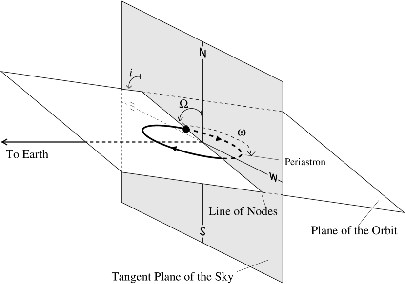
Figure 2.— Geometry of the binary system, showing position angle of ascending node, $\Omega$, inclination, $i$, and angle of periastron, $\omega$. The black dot indicates the ascending node.

Figure 3.— Shapiro delay in the timing residuals of PSR J1713+0747 as a function of orbital phase. (a) The Shapiro delay term is excluded from the model while the rest of the parameters are fixed at their best-fit values from Table 2. The solid curve shows the general relativistic delay predicted by equation 2. (b) The Shapiro term is excluded from the model but the other parameters are permitted to vary. (c) Shapiro delay is included in the model. The residuals in this panel are from the same timing fit as those in Figure 1b.

3.3. Orbital Kinematics Including Shapiro Delay

Orbital kinematics were incorporated into the timing model by means of the theory-independent representation of Damour & Deruelle (1986). Parameters of the orbital model include (1) five Keplerian orbital elements: orbital period, $P_{b}$; semi-major axis projected into the line of sight, $x=(a_{1}\sin i)/c$, where $a_{1}$ is the semi-major axis, $i$ the inclination angle, and $c$ the speed of light; eccentricity, $e$; angle of periastron, $\omega$; and time of periastron passage, $T_{0}$; (2) secular variations of the Keplerian elements, most notably the time derivative of $x$, denoted $\dot{x}$; (3) the orientation of the system, defined by the inclination of the orbit, $i$, where $0^{\circ}\leq i<180^{\circ}$, and the position angle of ascending node, $\Omega$, where $0^{\circ}\leq\Omega<360^{\circ}$ and $\Omega$ is defined north through east (see Figure 2); and (4) the masses of the pulsar and the secondary star, $m_{1}$ and $m_{2}$.

The masses and inclination are connected by the mass function,

$$f_{1}\equiv\frac{(m_{2}\sin i)^{3}}{(m_{1}+m_{2})^{2}}=\frac{x^{3}}{T_{\odot}}\left(\frac{2\pi}{P_{b}}\right)^{2},$$ (1)

where $T_{\odot}\!=\!GM_{\odot}/c^{3}\!=\!4.925\!\times\!10^{-6}\,$s. In the analysis below, we treat $i$ and $m_{2}$ as independent parameters in the timing model, and we use equation 1 to determine $m_{1}$.

According to general relativity, pulses are retarded as they propagate through the gravitational potential well of the secondary. For a nearly circular orbit, this Shapiro delay is

$$\Delta t_{s}=-2\,m_{2}\,T_{\odot}\ln[1-\sin{i}\sin(\phi+\omega)],$$ (2)

where $\phi$ is the orbital phase. In principle, measurement of the Shapiro delay yields $m_{2}$ and $\sin i$. In practice, unless $\sin i\sim 1$, the Shapiro delay is highly covariant with $x$ in the timing fit and hence difficult to measure. Nevertheless, as shown in Figure 3, the Shapiro delay can be clearly distinguished in the PSR J1713+0747 data. The constraints on $m_{2}$ and $i$ that arise from this measurement are quantified in §4. Since $0^{\circ}\leq i<180^{\circ}$ (see Figure 2), there in an ambiguity in deriving $i$ from $\sin i$ in equation 2, because both $i$ and $180^{\circ}\!-\!i$ are solutions. The resolution of this ambiguity is discussed below.

3.4. Projection Effects due to Proper Motion

Proper motion of a binary system results in secular changes in $\omega$ and $x$ (Kopeikin 1996). For a nearly circular orbit, a secular change in $\omega$ is indistinguishable from a small perturbation of the orbital period, and hence is unmeasurable. In contrast, the secular change in $x$ is significant. The time derivative of $x$, $\dot{x}$, is given by

$$\frac{\dot{x}}{x}=\mu\,\cot i\,\sin(\theta_{\mu}-\Omega),$$ (3)

where $\mu$ and $\theta_{\mu}$ are the magnitude and position angle of the proper motion, respectively. In effect, $i$ is determined by the Shapiro delay (§3.3), and $\Omega$ is then constrained by the $\dot{x}$ measurement. Solving equation 3 for $\Omega$ yields two possible values for each of the two values of $i$ (§3.3). Thus there are four distinct binary orientations (combinations of $i$ and $\Omega$) allowed by the Shapiro delay and $\dot{x}$ measurements.

3.5. Annual-Orbital Parallax

The Earth’s annual motion about the solar system barycenter changes the line-of-sight to the binary system and perturbs the binary parameters $x$ and $\omega$, an effect known as annual-orbital parallax (Kopeikin 1995; van Straten et al. 2001; van Straten & Bailes 2003). We incorporated annual-orbital parallax into the timing model by perturbing the values of $x$ and $\omega$ before calculating pulse arrival time delays using a standard orbital model. The perturbation formulae are given by Kopeikin (1995); we summarize them here. The position of the Earth relative to the solar system barycenter is given by the vector X, Y, Z. The pulsar position is right ascension $\alpha$ and declination $\delta$. Define

$$\begin{array}[]{c}\Delta_{\rm I0}=-X\sin\alpha+Y\cos\alpha,\\ \Delta_{\rm J0}=-X\sin\delta\cos\alpha-Y\sin\delta\sin\alpha+Z\cos\delta.\end{array}$$ (4)

These are the east and north motions of the Earth in a coordinate system parallel to the plane of the sky. The observed values of $x$ and $\omega$ are perturbed from their intrinsic values by

$$x_{\rm obs}=x_{\rm int}\left[1-\frac{\cot i}{d}(\Delta_{\rm I0}\cos\Omega-\Delta_{\rm J0}\sin\Omega)\right],$$ (5)

and

$$\omega_{\rm obs}=\omega_{\rm int}-\frac{\csc i}{d}(\Delta_{\rm I0}\sin\Omega+\Delta_{\rm J0}\cos\Omega).$$ (6)

Figure 4.— The effect of annual-orbital parallax on the timing solution is shown by displaying the difference in goodness of fit, $\Delta\chi^{2}$, as a function of position angle of ascending node. The value $\Delta\chi^{2}=0$ corresponds to the best timing model without annual-orbital perturbations. The 95% confidence range of $\Omega$ is indicated.

We found the annual-orbital perturbation of $x$ to have only a marginal effect on the timing of PSR J1713+0747, and no useful measurements can be derived from it. (Nevertheless, the $x$ perturbation was included in the timing model, since it introduced no additional degrees of freedom.) On the other hand, the perturbations of $\omega$ are sufficiently large that incorporating them into the timing model significantly improves the goodness of the timing fit. Figure 4 shows the $\chi^{2}$ values for fits with and without the annual-orbital parallax perturbations. In these fits, $m_{1}$, $i$, $\dot{x}$, and $\Omega$ were treated as independent parameters, unconstrained by equation 3; hence the best-fit range of $\Omega$ in Figure 4 differs somewhat from that given in §4.

As a practical matter, for PSR J1713+0747 the annual-orbital parallax does little to improve the precision of the timing parameter measurements (since $i$ and $\Omega$ are better measured by Shapiro delay and $\dot{x}$). However, it allows the fourfold ambiguity in $i$ and $\Omega$ to be broken, picking out one distinct orientation of the orbit.

Figure 5.— Probability distribution functions for values of $\Omega$, $m_{1}$, $m_{2}$, and $\cos i$.

Table 2Timing Model Parameters

Measured Quantities
Right Ascension, $\alpha$ (J2000)	$17^{\rm h}13^{\rm m}49\fs 5305335(6)$
Declination, $\delta$ (J2000)	$+07^{\circ}47\arcmin 37\farcs 52636(2)$
Total proper motion, $\mu$ (mas yr-1)	6.297(7)
Position angle of proper motion, $\theta_{\mu}$	128$\fdg$66(7)
Parallax, $\pi$ (mas)	0.89(8)
Rotation frequency, $\nu_{0}$ (s-1)	218.8118439157321(3)
First derivative of $\nu_{0}$, $\nu_{1}$ (s-2)	$-4.0835(2)\times 10^{-16}$
Epoch, $t_{0}$ (MJD [TDB])	52000.0
Dispersion Measure, DM0 (pc cm-3)	15.9960
Orbital period, $P_{b}$ (days)	67.8251298718(5)
Projected semi-major axis, $x$ (lt-s)	32.34242099(2)
Eccentricity, $e$	0.0000749406(13)
Time of periastron passage, $T_{0}$ (MJD [TDB])…	51997.5784(2)
Angle of periastron, $\omega$ (deg)	176.1915(10)
Cosine of inclination angle, $\cos i$	$0.31(3)$
Position angle of ascending node, $\Omega$ (deg)	$87(6)$
Companion mass, $m_{2}$ (M⊙)	$0.28(3)$
Measured Upper Limits
First derivative of DM, DM1 (pc cm-3 yr-1)	$0(2)\times 10^{-5}$
First derivative of $\omega$, $\dot{\omega}$ (deg yr-1)	$6(4)\times 10^{-4}$
First derivative of ${P_{b}}$, $\dot{P}_{b}$	$0(6)\times 10^{-13}$
Derived Quantities
Proper motion in $\alpha$, $\mu_{\alpha}=\dot{\alpha}\cos\delta$ (mas yr-1)	4.917(4)
Proper motion in $\delta$, $\mu_{\delta}=\dot{\delta}$ (mas yr-1)	$-$3.933(10)
Galactic longitude, $l$	$28\fdg 748$
Galactic latitude, $b$	$25\fdg 222$
Distance, $d$ (kpc)	$1.1(1)$
Rotation period, ${P}$ (s)	0.004570136525082781(6)
Observed rotation period derivative, $\dot{P}_{\rm obs}$	$8.5288(3)\times 10^{-21}$
Intrinsic rotation period derivative, $\dot{P}_{\rm int}$	$8.1\times 10^{-21}$
Characteristic age, $\tau$ (yr)	$8\times 10^{9}$
Magnetic field, $B_{0}$ (G)	$1.9\times 10^{8}$
Mass function, $f_{1}$ (M⊙)	$0.0078962167$
Pulsar mass, $m_{1}$ (M⊙)	$1.3(2)$
First derivative of $x$, $\dot{x}$ ($10^{-15}$)	6.7(2)

4. Timing Analysis: Parameter Values

We fit the measured TOAs to a timing model incorporating the phenomena described in §3. We used a hybrid procedure to determine the timing parameters and their uncertainties. Standard least-squares methods are adequate for fitting most of the quantities in the timing model. However, for the orientation and mass parameters, $i$, $\Omega$, and $m_{2}$, the $\chi^{2}$ surfaces are not ellipsoidal in the parameter space of interest. To investigate the allowed ranges of these parameters (and, ultimately, the other parameters as well), we analyzed timing solutions over a uniformly sampled three dimensional grid of trial values of $\cos i$, $m_{2}$, and $\Omega$, in the vicinity of the $\chi^{2}$ minimum. For each combination of $\cos i$, $m_{2}$, and $\Omega$, we calculated $\dot{x}$, the Shapiro delay parameters, and the annual-orbital perturbation corrections, according to equations 2, 3, 5, and 6. We then performed a timing fit, in which these quantities held fixed while all other parameters were allowed to vary. We recorded the resulting values of $\chi^{2}$ for each grid point.

The minimum $\chi^{2}$ timing solution is at $\cos i=0.31$, $m_{2}=0.28$ M_⊙, and $\Omega=87^{\circ}$. The parameters corresponding to this solution are summarized in Table 2. Our results show good agreement with the less precise results of van Straten & Bailes (2003).

We used a statistically rigorous procedure to calculate probability distribution functions (PDFs) for the individual quantities $\cos i$, $m_{2}$, $\Omega$, and $m_{1}$ and their corresponding uncertainties in table 2. The procedure is a straightforward three-dimensional extension of the Bayesian algorithm described in appendix A of Splaver et al. (2002). We assigned a probability to each grid point based on the difference between its $\chi^{2}$ and the minimum $\chi^{2}$ on the grid. After suitable normalization, we summed the probabilities of all points associated with a given range of $m_{1}$ (or $m_{2}$, $\cos i$, or $\Omega$) to calculate the PDF.

In effect, we are incorporating a uniform prior distribution in $\cos i$, $\Omega$, and $m_{2}$. The uniform distributions in $\cos i$ and $\Omega$ correspond to the probability distributions for the angular momentum vectors of randomly oriented orbits, while the uniform distribution of $m_{2}$ is simply an ad hoc assumption.

The calculated PDFs are given in Figure 5. They yield the 68% confidence estimates given in Table 2, most notably $m_{1}=1.3\pm 0.2\,{\rm M}_{\odot}$ and $m_{2}=0.28\pm 0.03\,{\rm M}_{\odot}$. The 95% confidence estimates on the masses are $m_{1}=1.3_{-0.3}^{+0.4}\,{\rm M}_{\odot}$ and $m_{2}=0.28^{+0.06}_{-0.04}\,{\rm M}_{\odot}$.

The interdependence between these parameters is show in the multidimensional confidence plots in Figures 6 and 7. To produce Figure 6, we summed normalized probabilities across all values of $\Omega$ to yield a two dimensional probability distribution in $\cos i$ and $m_{2}$. The contours enclose 68% and 95% of the probability distribution in this space. In Figure 7 we show representative “slices” in constant $\Omega$ of the regions enclosing 68% and 95% of the three dimensional grid.

5. Discussion

5.1. Orbital Period–Core Mass Relation

5.1.1 Testing the Relation

Binary evolution theory predicts a specific relationship between the orbital period, $P_{b}$, of an evolved neutron star–white dwarf binary and the secondary mass, $m_{2}$, which is presumed to be equal to the helium core of the progenitor of the secondary. Measured values of $m_{2}$ can be used to test this relation. Figure 8 shows the relations derived from binary evolution tracks calculated by Tauris & Savonije (1999) and Podsiadlowski et al. (2002). The latter curves are the median and upper values of $m_{2}$ of Rappaport et al. (1995), which provide good bounds on the tracks of Pfahl et al. (2002) (P. Podsiadlowski, private communication). The models are in good agreement with the measured values.

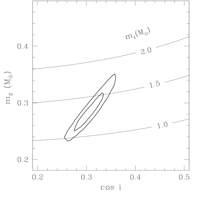
Figure 6.— Contours of 68% and 95% confidence intervals in $\cos i-m_{2}$ space.

5.1.2 Implications of the Relation for PSR J1713+0747 System Masses

If, rather than using timing measurements to test the orbital period–core mass relation, we accept this relation as correct, than we can use it to refine the range of pulsar mass allowed by the timing data. For the orbital period of J1713+0747, Tauris & Savonije (1999) calculate the secondary mass to be $0.31\,{\rm M}_{\odot}<m_{2}<0.34\,{\rm M}_{\odot}$, with the lower end of this range for a population I progenitor and the higher end for a population II progenitor. Pfahl et al. (2002) give a similar range, $0.30\,{\rm M}_{\odot}<m_{2}<0.35\,{\rm M}_{\odot}$ (again using the higher end of the range of Rappaport et al. 1995).

Repeating the statistical analysis of timing solutions on a $\cos i-m_{2}-\Omega$ as in § 4, but restricting $m_{2}$ to the range $0.30\,{\rm M}_{\odot}<m_{2}<0.35\,{\rm M}_{\odot}$ yields a value of $m_{1}=1.53_{-0.06}^{+0.08}$ (68% confidence).

5.2. Neutron Star Mass

Masses of pulsars and secondary stars in neutron star–neutron star binaries all fall within the range 1.25 to 1.44 ${\rm M}_{\odot}$. This is near the minimum mass for neutron star formation; the maximum mass is not known, and may range up to 3 ${\rm M}_{\odot}$ (see Lattimer & Prakash 2004, for a review). Because binary systems which evolve into pulsar–white dwarf binaries like the PSR J1713+0747 system undergo extended periods of mass transfer, the pulsars in these systems might be expected to be heavier than those in neutron star–neutron star binaries.

Thorsett & Chakrabarty (1999) studied the entire binary pulsar population and found it to be consistent with a narrow Gaussian distribution with mean 1.35 ${\rm M}_{\odot}$ and width 0.04 ${\rm M}_{\odot}$. Their calculation included a statistical analysis of the pulsar–white dwarf population, under the assumption that the binaries were randomly oriented in space and that the orbital period-core mass relation held, and they found that these pulsars could be drawn from the same mass distribution as pulsars in neutron star–neutron star binaries.

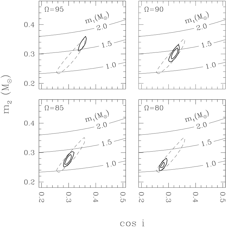
Figure 7.— Contours of 68% and 95% confidence intervals in $\cos i-m_{2}-\Omega$ space. Four slices of constant $\Omega$ are shown; in each, the intersection of the slice with the 68% and 95% confidence region is given. The slice at $\Omega=95^{\circ}$ intersects only the 95% region. The dashed line corresponds to the 95% confidence region after marginalizing over all values of $\Omega$ (cf. Figure 6).

The measured mass of PSR J1713+0747 based on observations alone, $m_{1}=1.3\pm 0.2\,{\rm M}_{\odot}$, is in excellent agreement with the 1.35 ${\rm M}_{\odot}$ value. In contrast, the mass derived when the orbital period-core mass constraint is imposed, $m_{1}=1.53_{-0.06}^{+0.08}\,{\rm M}_{\odot}$, implies a significantly heavier neutron star, perhaps having accreted $\approx 0.2$ ${\rm M}_{\odot}$ if initially formed at $1.35$ ${\rm M}_{\odot}$. There are two other pulsar–helium white dwarf binaries with well measured Shapiro delays, PSRs J0437$-$4715 and B1855+09, which have pulsar masses $1.58\pm 0.18\,{\rm M}_{\odot}$ and $1.50^{+0.26}_{-0.14}\,{\rm M}_{\odot}$, respectively (van Straten et al. 2001; Kaspi et al. 1994). On the other hand, PSR J2019+2425, in a similar system, shows a lack of a detectable Shapiro delay and observed secular changes which imply an upper limit of 1.51 ${\rm M}_{\odot}$ and a median likelihood value of 1.33 ${\rm M}_{\odot}$ (Nice et al. 2001). The uncertainties on all of these measurements are frustratingly large; the question of the distribution of pulsars masses in these systems remains open.

5.3. Parallax, Distance, and Velocity

Because the solar wind introduces annual perturbations on the pulse arrival times, the solar wind electron density parameter, $n_{0}$, is highly covariant with parallax, $\pi$, and position, $\alpha$ and $\delta$, in the pulse arrival time model. For $\pi$, the measurement uncertainty using any fixed solar wind model is $\pm 0.05$ mas, while the uncertainty due to the poor constraint on $n_{0}$ is $\pm 0.06$ mas. We combine these uncertainties in quadrature to find $\pi=0.89\pm 0.08$ mas. As a check, a special timing fit was done incorporating only days on which multifrequency observations were made, and fitting for a separate value of DM on each day on which observations were made, yields a parallax of $0.93\pm 0.24$, consistent with our preferred value. The parallax measurement corresponds to a distance of $d=1.1\pm 0.1$ kpc.

For PSR J1713+0747’s measured value of DM, the NE2001 model of the Galactic electron density (Cordes & Lazio 2002) gives a distance of 0.9 kpc, in good agreement with the parallax measurement.

Right ascension and declination are also highly covariant with $n_{0}$; their uncertainties quoted in Table 2 were calculated in the same manner as the parallax uncertainty.

It is well established that millisecond pulsars have substantially smaller velocities than the bulk pulsar population, with a mean transverse velocity of $85\pm 13$ km s^-1 (Cordes & Chernoff 1997; Toscano et al. 1999; Nice & Taylor 1995). The transverse velocity of PSR J1713+0747, $V=\mu d=33\pm 3\rm{\,km\,s^{-1}}$, is small even by the standards of millisecond pulsars.

Figure 8.— Theoretical $m_{2}-P_{b}$ relation and measured white dwarf masses in pulsar–white dwarf binaries. Measured masses are from van Straten et al. (2001) (J0437$-$4715), Kaspi et al. (1994) (B1855+09), and this work (J1713+0747).

5.4. Kinematic Corrections to Spin Period Derivative; Age & Magnetic Field

The observed pulse period derivative, $\dot{P}_{\rm obs}=-\nu_{1}/\nu_{0}^{2}$, is biased away from its intrinsic value, $\dot{P}_{\rm int}$, by Doppler accelerations. Damour & Taylor (1991) analyzed this bias for orbital period derivatives; their work applies equally well to spin period derivatives. The observed and intrinsic quantities are related by

$$\dot{P}_{\rm int}=\dot{P}_{\rm obs}-\Delta\dot{P}_{\rm PM}-\Delta\dot{P}_{\rm rot}-\Delta\dot{P}_{\rm z},$$ (7)

where $\Delta\dot{P}_{\rm PM}=P\mu^{2}d/c$ is the bias due to proper motion; $\Delta\dot{P}_{\rm rot}=P({\bf a}_{\rm rot}\cdot{\bf n})/c$ is the bias due to the relative acceleration of pulsar and Earth in the Galactic plane, ${\bf a}_{\rm rot}$, projected into a unit vector pointing from Earth to pulsar, ${\bf n}$; and $\Delta\dot{P}_{\rm z}=P({\bf a}_{\rm z}\cdot{\bf n})/c$ is the bias due to the acceleration of the pulsar toward the galactic disk, ${\bf a}_{z}$, projected into the line-of-sight.

For PSR J1713+0747, we find $\Delta\dot{P}_{\rm PM}=0.46\times 10^{-21}$, $\Delta\dot{P}_{\rm rot}=0.22\times 10^{-21}$ and $\Delta\dot{P}_{\rm z}=-0.32\times 10^{-21}$, the latter calculated using the potential of Kuijken & Gilmore (1989). The net bias is $\Delta\dot{P}=0.44\times 10^{-21}$, so that we estimate the intrinsic period derivative to be $\dot{P}_{\rm int}=8.1\times 10^{-21}$.

The characteristic age of PSR J1713+0747 is $\tau=P/2\dot{P}_{\mathrm{int}}=8\mathrm{\,Gyr}$. This probably overestimates the true age of the pulsar. Hansen & Phinney (1998) obtain a considerably lower estimate by using the optical measurements of Lundgren, Foster, & Camilo (1996) to infer the age of the white dwarf to be 6.3 Gyr $<\tau<$ 6.8 Gyr.

A discrepancy between the characteristic age and the true age of a millisecond pulsar is not uncommon (e.g., Nice & Taylor 1995), and implies that the millisecond pulsar period immediately after spin-up was close to its present day value. It seems likely that millisecond pulsars form with periods of a few milliseconds (Backer 1998).

The surface magnetic field strength of the pulsar according to conventional assumptions is $B_{0}=3.2\times 10^{19}(P\dot{P}_{\mathrm{int}})^{1/2}\mathrm{\,G}=1.9\times 10^{8}\mathrm{\,G}$. This value is typical of millisecond pulsars.

5.5. Timing Noise

The PSR J1713+0747 timing data show timing noise. Analysis of the timing noise is complicated by the large gap in the data between 1994 and 1998 and because of the need to allow an offset in the arrival times before and after the gap. To analyze timing noise, we calculated residuals for a timing model fitting for only the pulsar spin-down parameters $\nu_{0}$ and $\nu_{1}$ and an arbitrary offset between the pre-1994 and post-1998 data. Astrometric and binary parameters were held fixed at the values derived from the whitened timing model fit. The results are shown in Figure 1a.

Timing noise can be quantified by the fractional stability statistic $\sigma_{z}$, an adaptation of the “Allan variance” statistic with modifications appropriate for pulsar timing (Matsakis et al. 1997). In essence, $\sigma_{z}$ for time interval $\tau$ is calculated by dividing the post-fit residual arrival times, $r(t)$, into intervals spanning length $\tau$, and fitting third order polynomials over each interval, $r(t)=\Sigma_{i=0}^{3}c_{i}(t\!-\!t_{0})^{i}$. The first three terms of the polynomial are accounted for by the pulsar spin-down model. The final term, $c_{3}$, is a measure of timing noise. The statistic is calculated by appropriately scaling the root-mean-square value of $c_{3}$ from all intervals of a given length: $\sigma_{z}(\tau)=(1/2\sqrt{5})\tau^{2}\left<c_{3}^{2}\right>^{1/2}$.

Figure 9 shows $\sigma_{z}(\tau)$ of PSR J1713+0747 as calculated from the residual pulse arrival times shown in Figure 1a. For uniformly sampled data exhibiting white noise, $\sigma_{z}$ would fall off as $\tau^{-3/2}$; this is the behavior observed on all but the longest time scale. At $\tau=12$ yr, timing noise is evident. Because of the arbitrary offset fit between the 1994 and 1998 data, it is possible that the calculated value of $\sigma_{z}(\tau)$ underestimates its true value on the longest time scale.

The physical mechanism underlying timing noise is not known. Arzoumanian et al. (1994) studied a large collection of pulsars using a statistic, $\Delta_{8}$, which is the logarithm of a scaled version of $\sigma_{z}(\tau)$ at $\tau=10^{8}\,{\rm s}\approx 3\,{\rm yr}$ (see also Backer 2004). From Figure 9, it is evident that at a time scale of 3 yr, $\sigma_{z}$ is dominated by measurement noise, so the measured values are upper limits on the intrinsic irregularities in the pulsar signal. Estimating $\log\sigma_{z}(3\,{\rm yr})\lesssim-14.2$ for PSR J1713+0747, we calculate $\Delta_{8}\lesssim-5.6$. Arzoumanian et al. (1994) found $\Delta_{8}$ to be correlated with pulse period derivative according to $\Delta_{8}=6.6+0.6\log\dot{P}$. This formula predicts $\Delta_{8}=-5.5$ for PSR J1713+0747, close to the observed upper limit. Thus the rotational stability of J1713+0747 is as good (or better) than expected, despite the long-term timing noise.

Figure 9.— Noise statistic $\sigma_{z}$ as a function of time scale, $\tau$. Gaussian noise would result in $\sigma_{z}\sim\tau^{-3/2}$, parallel to the dashed line. The upturn at $\tau>2\,$yr is indicative of timing noise with a red spectrum. The $\sigma_{z}$ values at the longest time scales may be affected by the presence of a 4-year gap in the data and by the need for an arbitrary offset between pre- and post-gap data; however, we believe the upward trend at $\tau>2$ yr to be qualitatively correct.

5.6. Solar System Ephemerides

As discussed above, we used the DE405 solar system ephemeris to reduce the pulse arrival times to the solar system barycenter. To reduce pulse arrival times measured with uncertainty of only $\sim 200$ ns, the Earth’s position with respect to the barycenter must be known with precision $60$ m. We analyzed our data with both DE405 and its predecessor, DE200. To compare the two ephemerides, we performed timing fits on the the post-1998 data. Excluding the earlier data from these tests allowed us to avoid problems stemming from the arbitrary offset between the earlier and later data. Using each ephemeris, we fit the data to a full timing model, fitting for all the standard parameters but not allowing pulse frequency derivatives above $\nu_{1}$ (i.e., no timing noise terms). The results are shown in Figure 10. The DE405 ephemeris clearly gives a better fit. The differences in timing quality are easily explained by differences in the ephemerides themselves, particularly the incorporation of improved measurements of outer planet masses into DE405 (E. M. Standish, private communication).

Figure 10.— Residual arrival times from timing models for 1998-2004 data calculated using (a) the DE200 solar system ephemeris and (b) the DE405 solar system ephemeris.

5.7. Testing Strong Field Gravity

PSR J1713+0747 is one of several long-orbit, low-eccentricity binary pulsars which have been used to set limits on violations of equivalence principles (Damour & Schäfer 1991; Wex 1997; Bell & Damour 1996; Wex 2000). The relevant observational signatures depend on the orientations of the binary systems under study, something not usually known; hence, probabilistic arguments have been used to constrain equivalence principle violations based on observations of several pulsars. In contrast, we have established the orientation ($i$ and $\Omega$) to PSR J1713+0747, and we have measured its distance as well. This allows us to set the first absolute limits both on violation of the Strong Equivalence Principle (SEP) and on the magnitude of the strong-field equivalent of the Parametrized Post-Newtonian (PPN) parameter $\hat{\alpha}_{3}$.

5.7.1 The Strong Equivalence Principle

If the SEP were violated, objects with different fractional mass contributions from self-gravitation would fall differently in an external gravitational field. This is quantified by the parameter $\eta$, defined through $m_{g}/m_{i}=1+\eta E_{g}/mc^{2}$, where $m_{g}$, $m_{i}$, and $E_{g}$ are the gravitational mass, inertial mass, and gravitational self-energy of a body. Nonzero values of $\eta$ would result in the polarization of binary orbits (Nordtvedt 1968). Lunar laser ranging experiments set limits on the polarization of the Earth-Moon orbit in the gravitational field of the Sun, constraining $|\eta|$ to be less than 0.001 (Dickey et al. 1994; Will 2001). In the case of a pulsar–white-dwarf binary, the orbit would be polarized in the direction of the gravitational pull of the Galaxy. The parameter to be constrained, $\Delta$, is similar to $\eta$, but without the requirement of linear dependence on $E_{g}/mc^{2}$. It is defined for an individual body, $a$, by $(m_{g}/m_{i})_{a}=1+\Delta_{a}$; dynamics of a binary orbit depend on the difference $\Delta=\Delta_{1}-\Delta_{2}$ between the two objects (see Damour & Schäfer 1991, for full details).

The (small) “forced” eccentricity ${\bf e}_{F}$ of the orbit induced by the SEP violation may be written as:

$$|{\bf e}_{F}|=\frac{1}{2}\frac{\Delta{\bf g}_{\perp}c^{2}}{FG\,(m_{1}+m_{2})(2\pi/P_{\rm b})^{2}},$$ (8)

where ${\bf g}_{\perp}$ is the projection of the Galactic gravitational field onto the orbital plane and, in General Relativity, $F=1$. This forced eccentricity may be comparable in magnitude to the “natural” eccentricity ${\bf e}_{R}(t)$ of the system, which by definition rotates at the rate of the advance of periastron and may, at any time, be oriented in such a way as to nearly cancel the forced eccentricity. Defining the angle between these two vectors as $\theta$, Wex (1997) writes the inequality:

$$|{\bf e}_{F}|\leq e\xi_{1}(\theta),\,\,\,\,\,\xi_{1}(\theta)=\left\{\begin{array}[]{r@{\quad:\quad}l}1/\sin\theta&\theta\in[0,\pi/2)\\ 1&\theta\in[\pi/2,3\pi/2]\\ -1/\sin\theta&\theta\in(3\pi/2,2\pi)\end{array}\right.,$$ (9)

where $e$ is the observed eccentricity.

The projection of ${\bf g}$ onto the orbital plane can be written as (Damour & Schäfer 1991):

$$|{\bf g}_{\perp}|=|{\bf g}|[1-(\cos i\cos\lambda+\sin i\sin\lambda\sin(\phi_{\rm g}-\Omega))^{2}]^{1/2},$$ (10)

where $\phi_{\rm g}$ is the angle of the projection of ${\bf g}$ onto the plane of the sky (effectively a celestial position angle, defined north through east as for $\Omega$), and $\lambda$ is the angle between ${\bf g}$ and the line from the pulsar to the Earth. The value of $|{\bf g}|$ can be determined from models of the Galactic potential (e.g., Kuijken & Gilmore 1989) and the Galactic rotation curve; for a pulsar out of the Plane of the Galaxy, $\lambda$ is given by

$$\cos\lambda=\frac{-R_{0}^{2}+d^{2}+R_{1}^{2}+z^{2}}{2\,d\,\sqrt{R_{1}^{2}+z^{2}}},$$

where $R_{1}=(R_{0}^{2}+(d\cos b)^{2}-2R_{0}d\cos b\cos l)^{1/2}$ is the Galactic radius of the pulsar, $R_{0}$ is the distance from the Earth to the Galactic center, $z$ is the distance from the pulsar to the Galactic plane, and $l$ and $b$ are the Galactic coordinates of the pulsar.

Historically, both $\theta$ and $\Omega$ have been completely unknown for the pulsars used to test for violation of the SEP, and the tests have therefore made statistical arguments, assuming both angles to be uniformly distributed between 0 and $2\pi$ (e.g., Damour & Schäfer 1991). The masses have also been poorly constrained and thus averages over likely model populations were also needed (Wex 2000). Following these procedures, an ensemble of long-orbit pulsars yields a limit of $|\Delta|<0.009$ at 95% confidence.

With both masses and the angle of the line of nodes well-constrained for PSR J1713+0747, a single, more robust limit on violation of the SEP becomes possible. Because of the complicated dependence of $\Delta$ on the pulsar distance, as well as the asymmetric distribution of allowed masses, we obtain the limit via Monte Carlo simulation, assuming the parallax to be normally distributed and $\theta$ to be uniformly distributed, and sampling the allowed $m_{2}$–$\cos i$–$\Omega$ range according the probability distribution derived from the $\chi^{2}$ grid discussed above. We find that $|\Delta|<0.013$ at 95% confidence. This is nearly as good a limit as could be expected from this pulsar, as just over 90% of the Galactic acceleration vector is parallel to the plane of the orbit. The most stringent test of SEP violation, however, continues to rely on an ensemble of pulsars.

5.7.2 Post-Newtonian Parameter $\hat{\alpha}_{3}$

The parameter $\alpha_{3}$ is one of ten PPN parameters formulated to describe departures from General Relativity in the weak-field limit (Will & Nordtvedt 1972). Its strong-field analog, $\hat{\alpha_{3}}$, can be tested by pulsar timing (Damour & Esposito-Farèse 1992, 1996). A non-zero $\hat{\alpha}_{3}$ would imply both violation of local Lorentz invariance and non-conservation of momentum (e.g., Will 2001). For a pulsar–white-dwarf binary, the net effect would be to cause an acceleration of the binary system given by (Bell & Damour 1996):

$${\bf a}_{\hat{\alpha}_{3}}=\frac{1}{6}\hat{\alpha}_{3}c_{\rm p}{\bf w}\times{\bf\Omega}_{\rm Sp},$$ (11)

where ${\bf\Omega}_{\rm Sp}$ is the spin angular frequency of the pulsar ($|\Omega_{\rm Sp}|=2\pi\nu_{0}$), ${\bf w}$ is the absolute velocity of the system, and $c_{\rm p}$ denotes the compactness of the pulsar, roughly the fraction of its mass contained in gravitational self-energy. An approximate expression for the compactness is $c_{\rm p}\simeq 0.21\,m_{1}/M_{\odot}$ (Damour & Esposito-Farèse 1992). As above, this acceleration will induce a “forced” eccentricity in the orbit, given by

$$|{\bf e}_{F}|=\hat{\alpha}_{3}\frac{c_{\rm p}|{\bf w}|}{24\pi}\frac{P_{\rm b}^{2}}{P}\frac{c^{2}}{G(m_{1}+m_{2})}\sin\beta,$$ (12)

where $\beta$ is the angle between ${\bf w}$ and ${\bf\Omega}_{\rm Sp}$, and $P$ is the spin period of the pulsar: $P=2\pi/\Omega_{\rm Sp}$. Using an ensemble of pulsars and assuming random distributions of the orbital inclinations, Wex (2000) found a limit of $|\hat{\alpha}_{3}|<1.5\times 10^{-19}$. To calculate the limit imposed by PSR J1713+0747, we again proceed via Monte Carlo simulation, sampling the parameters as described above. We assume that the pulsar spin and orbital angular momenta have been aligned during the spin-up episode that recycled the pulsar. Thus with the full orientation of the orbit known for each simulation point, we can easily calculate $\beta$ given any ${\bf w}$. This absolute velocity is taken to be in the reference frame of the Cosmic Microwave Background (CMB), and is calculated from the motion of the Solar System in the CMB reference frame (369 km/s toward $\alpha=11\fh 3$, $\delta=-7^{\circ}$; Fixsen et al. 1994) and the three dimensional velocity of the binary system relative to the Solar System. The radial component of this second velocity vector is unknown. We checked a range of radial velocities from $-200$ km/s and $+200$ km/s; for each simulation point, we adopted the value that gives the smallest projection of the total velocity onto the plane of the orbit. This value was always in the range $-60$ to +25 km/s. We thus arrived at an absolute 95%-confidence limit of $|\hat{\alpha}_{3}|<1.2\times 10^{-19}$. This is better than the limit derived from the ensemble of pulsars and, as it is less statistical in nature, it may be considered a robust true limit on $\hat{\alpha_{3}}$. Future refinement of the timing parameters will improve this limit somewhat, with the floor ultimately determined by the orbital geometry.

6. Conclusion

PSR J1713+0747 has lived up to its promise as one of the best pulsars for high precision timing, with 200 ns residual pulse arrival times attained on time scales of years, and residuals well under 2$\mu$s over the full 12-yr data set. Major findings include:

1. The pulsar mass is constrained to $m_{1}=1.3\pm 0.2\,{\rm M}_{\odot}$ by the measured Shapiro delay. If the secondary mass is restricted to values predicted by the theoretical orbital period-core mass relation, the pulsar mass is somewhat higher, $m_{1}=1.53_{-0.06}^{+0.08}$.

2. The parallax is $\pi=0.89\pm 0.08$ mas, corresponding to a distance of $1.1\pm 0.1$ kpc. This is consistent with predictions based on the pulsar’s dispersion measure.

3. The orientation of the binary has been fully determined by the combined measurements of Shapiro delay and of perturbations of orbital elements due to relative Earth-pulsar motion. The orientation and very low ellipticity of the orbit lead to an improved constraint on deviations from general relativity.

The timing precision attainable on short time scales appears to be limited by measurement precision. There is every reason to expect timing precision to improve in the coming years as a new generation of wide bandwidth coherent dedispersion systems are employed at radio telescopes, directly resulting in more precise measurement of the Shapiro delay and hence of the pulsar and white dwarf masses.

References

- Arzoumanian et al. (1994) Arzoumanian, Z., Nice, D. J., Taylor, J. H., & Thorsett, S. E. 1994, ApJ, 422, 671
- Backer (1998) Backer, D. C. 1998, ApJ, 493, 873
- Backer (2004) Backer, D. C. 2004, in Binary Radio Pulsars, ed. F. A. Rasio & I. H. Stairs (San Francisco: Astronomical Society of the Pacific), in press
- Bell & Damour (1996) Bell, J. F. & Damour, T. 1996, Classical Quantum Gravity, 13, 3121
- Bureau International des Poids et Mesures (2003) Bureau International des Poids et Mesures. 2003, ftp://ftp2.bipm.org/pub/tai/scale/ttbipm.03
- Camilo et al. (1994) Camilo, F., Foster, R. S., & Wolszczan, A. 1994, ApJ, 437, L39
- Cordes & Chernoff (1997) Cordes, J. M. & Chernoff, D. F. 1997, ApJ, 482, 971
- Cordes & Lazio (2002) Cordes, J. M. & Lazio, T. J. W. 2002, http://xxx.lanl.gov/abs/astro-ph/0207156
- Damour & Deruelle (1986) Damour, T. & Deruelle, N. 1986, Ann. Inst. H. Poincaré (Physique Théorique), 44, 263
- Damour & Esposito-Farèse (1996) Damour, T. & Esposito-Farèse, G. 1996, Phys. Rev. D, 53, 5541
- Damour & Esposito-Farèse (1992) Damour, T. & Esposito-Farèse, G. 1992, Classical Quantum Gravity, 9, 2093
- Damour & Schäfer (1991) Damour, T. & Schäfer, G. 1991, Phys. Rev. Lett., 66, 2549
- Damour & Taylor (1991) Damour, T. & Taylor, J. H. 1991, ApJ, 366, 501
- Dickey et al. (1994) Dickey, J. O., Bender, P. L., Faller, J. E., Newhall, X. X., Ricklefs, R. L., Ries, J. G., Shelus, P. J., Veillet, C., Whipple, A. L., Wiant, J. R., Williams, J. G., & Yoder, C. F. 1994, Science, 265, 482
- Fixsen et al. (1994) Fixsen, D. J., Cheng, E. S., Cottingham, D. A., Eplee, R. E., Isaacman, R. B., Mather, J. C., Meyer, S. S., Noerdlinger, P. D., Shafer, R. A., Weiss, R., Wrigth, E. L., Bennett, C. L., Boggess, N. W., Kelsall, T., Moseley, S. H., Silverberg, R. F., Smoot, G. F., & Wilkinson, D. T. 1994, ApJ, 420, 445
- Foster et al. (1993) Foster, R. S., Wolszczan, A., & Camilo, F. 1993, ApJ, 410, L91
- Hansen & Phinney (1998) Hansen, B. M. S. & Phinney, E. S. 1998, MNRAS, 294, 569
- Irwin & Fukushima (1999) Irwin, A. W. & Fukushima, T. 1999, A&A, 348, 642
- Issautier et al. (2001) Issautier, K., Hoang, S., Moncuquet, M., & Meyer-Vernet, N. 2001, Space Sci. Rev., 97, 105
- Kaspi et al. (1994) Kaspi, V. M., Taylor, J. H., & Ryba, M. 1994, ApJ, 428, 713
- Kopeikin (1995) Kopeikin, S. M. 1995, ApJ, 439, L5
- Kopeikin (1996) —. 1996, ApJ, 467, L93
- Kuijken & Gilmore (1989) Kuijken, K. & Gilmore, G. 1989, MNRAS, 239, 571
- Lattimer & Prakash (2004) Lattimer, J. H. & Prakash, M. 2004, Science, 304, 536
- Lommen et al. (2003) Lommen, A. N., Backer, D. C., Splaver, E. M., & Nice, D. J. 2003, in Radio Pulsars, ed. M. Bailes, D. J. Nice, & S. Thorsett (San Francisco: Astronomical Society of the Pacific), 81
- Lundgren et al. (1996) Lundgren, S. C., Foster, R. S., & Camilo, F. 1996, in Pulsars: Problems and Progress, IAU Colloquium 160, ed. S. Johnston, M. A. Walker, & M. Bailes (San Francisco: Astronomical Society of the Pacific), 497
- Matsakis et al. (1997) Matsakis, D. N., Taylor, J. H., & Eubanks, T. M. 1997, A&A, 326, 924
- Nice et al. (2001) Nice, D. J., Splaver, E. M., & Stairs, I. H. 2001, ApJ, 549, 516
- Nice et al. (2003) Nice, D. J., Splaver, E. M., & Stairs, I. H. 2003, in Radio Pulsars, ed. M. Bailes, D. J. Nice, & S. Thorsett (San Francisco: Astronomical Society of the Pacific), 75
- Nice et al. (2004) Nice, D. J., Stairs, I. H., & Splaver, E. M. 2004, in Binary Radio Pulsars, ed. F. A. Rasio & I. H. Stairs (San Francisco: Astronomical Society of the Pacific), in press
- Nice & Taylor (1995) Nice, D. J. & Taylor, J. H. 1995, ApJ, 441, 429
- Nordtvedt (1968) Nordtvedt, K. 1968, Phys. Rev., 170, 1186
- Pfahl et al. (2002) Pfahl, E., Rappaport, S., & Podsiadlowski, P. 2002, ApJ, 573, 283
- Podsiadlowski et al. (2002) Podsiadlowski, P., Rappaport, S., & Pfahl, E. D. 2002, ApJ, 565, 1107
- Rappaport et al. (1995) Rappaport, S., Podsiadlowski, P., Joss, P. C., DiStefano, R., & Han, Z. 1995, MNRAS, 273, 731
- Splaver et al. (2002) Splaver, E. M., Nice, D. J., Arzoumanian, Z., Camilo, F., Lyne, A. G., & Stairs, I. H. 2002, ApJ, 581, 509
- Stairs et al. (2000) Stairs, I. H., Splaver, E. M., Thorsett, S. E., Nice, D. J., & Taylor, J. H. 2000, MNRAS, 314, 459
- Standish (1998) Standish, E. M. 1998, http://ssd.jpl.nasa.gov/iau-comm4/de405iom
- Standish (2004) —. 2004, A&A, 417, 1165
- Stinebring et al. (1992) Stinebring, D. R., Kaspi, V. M., Nice, D. J., Ryba, M. F., Taylor, J. H., Thorsett, S. E., & Hankins, T. H. 1992, Rev. Sci. Instrum., 63, 3551
- Tauris & Savonije (1999) Tauris, T. M. & Savonije, G. J. 1999, A&A, 350, 928