Simple route to non-Gaussianity in inflation

Abstract

We present a simple way to calculate non-Gaussianity in inflation using fully non-linear equations on long wavelengths with stochastic sources to take into account the short-wavelength quantum fluctuations. Our formalism includes both scalar metric and matter perturbations, combining them into variables which are invariant under changes of time slicing in the long-wavelength limit. We illustrate this method with a perturbative calculation in the single-field slow-roll case. We also introduce a convenient choice of variables to graphically present the full momentum dependence of the three-point correlator.

Introduction — The standard lore of inflation states that the statistical properties of its perturbations correspond to those of Gaussian random fields. Gaussianity is sometimes presented as a robust prediction regardless of any realisation in the context of a specific model. Such a statement may be adequate for comparing inflation with topological defects, since the latter are distinctly non-Gaussian, but its validity is related to the use of linear theory and is only approximate. Since gravity is inherently non-linear and the scalar fields responsible for inflation may have interacting potentials, some non-linearity will always be present and manifest itself as non-Gaussianity in the cosmic microwave background radiation (CMB). Hence the issue is not whether inflation is non-Gaussian, but how large the non-Gaussianity is. In an era of precision cosmology, it is potentially an additional observable to be sought in future CMB missions.

The current observational discriminants between inflationary models are the amplitude of the power spectrum, the spectral index, its running, and the tensor to scalar ratio ll , all calculated in linear theory. A priori, non-Gaussianity offers another quantity, characteristic of a model, which can be used as a discriminant. Different models are expected to exhibit a different amount and type of non-linearity and hence carry their own non-Gaussian signature. Naively, it is expected that any non-linearity will be very small given that linear fluctuations are small: an order of magnitude estimate is

$$\left(\frac{\Delta T}{T}\right)_{\mathrm{NL}}\sim f_{\mathrm{NL}}\left(\frac{\Delta T}{T}\right)^{2}_{\mathrm{L}}.$$ (1)

However, given the accuracy of future CMB missions, one could try to see whether such small non-linearities are observable. For example, the Planck satellite will be able to detect them, if $f_{\mathrm{NL}}\sim\mathcal{O}(1)$ komatsu .

The question of non-Gaussianity requires techniques beyond linear theory. Apart from early attempts to calculate it early_attempts , the issue attracted some attention recently after the promise of high quality CMB data from satellites like WMAP and Planck. The usual theoretical approach has been to expand the Einstein equations to second order acquaviva ; noh_and_hwang . An extensive survey of such techniques (including references) is provided in ng_review . A tree-level action treatment of interacting perturbations was given in mald .

In gp2 ; formalism we presented a new framework for calculating non-Gaussianity. It is valid in a very general multiple-field inflation setting, which includes the possibility of a non-trivial field metric. In this paper we illustrate that general formalism by applying it to the simple case of single-field inflation. Explicit calculations in the multiple-field case can be found in mf .

The formalism consists of a long-wavelength approximation coupled with a stochastic picture for the generation of perturbations on the relevant scales. It describes the evolution of variables which are invariant under changes of time slicing in the long-wavelength limit. These variables specify the inhomogeneous system, taking into account both matter and scalar metric perturbations, and are defined without recourse to the concept of a linear perturbation. The equations are formally very simple, yet they encode the full non-linear evolution on large scales. These stochastic equations offer a generalisation of currently existing stochastic approaches to the description of inflationary fluctuations stoch . They are suitable for a perturbative analytic treatment which is technically less complicated than perturbing the original Einstein equations. They are also well-suited as a basis for computer simulations which include the full non-linear evolution of the perturbations.

This paper is organised as follows. We start by summarising the general formalism of gp2 ; formalism , simplified to the single-field case. Using this we then analytically calculate the three-point correlator of the curvature perturbation for single-field slow-roll inflation, which would be zero in the Gaussian case. Our result is a completely explicit expression, containing the full momentum dependence. We introduce a convenient choice of variables to graphically present this momentum dependence. We also calculate the effects of the decaying mode. We conclude by discussing the results.

Basic formalism — A defining characteristic of inflation is the behaviour of the comoving Hubble radius $1/(aH)$, which shrinks quasi-exponentially. A mode with comoving wavenumber $k$ is called super-horizon when $k<aH$, and conversely sub-horizon when $k>aH$. The inflaton is taken to be in a vacuum state, defined such that sub-horizon modes approach the Minkowski vacuum for $k\mg aH$. After a mode exits the horizon, it is described by a classical probability distribution with a variance given by the power spectrum classicality . We will focus attention on the classical super-horizon regime and assume that the dynamics on these scales are adequately described by dropping from the equations all terms explicitly containing second-order spatial gradients long wavelength (i.e. the long-wavelength approximation). Then, focusing on scalar modes only, spacetime can be described by the metric

$$ds^{2}=-N^{2}(t,\mathbf{x})\mathrm{d}t^{2}+a^{2}(t,\mathbf{x})\mathrm{d}\mathbf{x}^{2},$$ (2)

with $a$ the local scale factor and $N$ the lapse function. The local expansion rate is defined as $H\equiv\dot{a}/(Na)$, where the dot denotes a derivative with respect to $t$. Here, we consider inflation to be driven by a single inflaton $\phi$. We also define two local slow-roll parameters by

$${\tilde{\epsilon}}(t,{\mathbf{x}})\equiv\frac{\kappa^{2}\Pi^{2}}{2H^{2}}\,,\qquad{\tilde{\eta}}(t,{\mathbf{x}})\equiv-3-\frac{\partial V/\partial\phi}{H\Pi}\,,$$ (3)

where $V$ is the potential, $\Pi\equiv\dot{\phi}/N$ and $\kappa^{2}\equiv 8\pi G=8\pi/m^{2}_{\rm pl}$.

The fact that we focus on scalar modes only is an approximation, since beyond linear theory, in general, scalar, vector, and tensor modes will mix. For complete consistency the spatial part of the metric in (2) should be multiplied by an $h_{ij}$ matrix with unit determinant, containing vector and tensor modes. However, in the long-wavelength approximation $h_{ij}$ would be non-dynamical, as shown for example in formalism . Moreover, at second order in the perturbations (which gives the leading-order non-Gaussianity), the scalar modes are only affected by the linear vector and tensor modes, the former of which are zero, while the latter are subdominant to the scalar modes. Hence it seems a good approximation to neglect vector and tensor modes to obtain a leading-order expression for non-Gaussianity. Vector and tensor modes will be investigated in future work.

Since we will be dealing with non-linearities, it is useful to describe inhomogeneity without resorting to the concept of a linear perturbation. In this case, it makes sense to consider the spatial gradient of quantities. In particular we will work with the following combination of spatial gradients:

$$\zeta_{i}(t,{\mathbf{x}})\equiv\partial_{i}\ln a(t,{\mathbf{x}})-\frac{\kappa}{\sqrt{2{\tilde{\epsilon}}(t,{\mathbf{x}})}}\,\partial_{i}\phi(t,{\mathbf{x}}),$$ (4)

which is invariant under changes of time slicing, up to second-order spatial gradients gp ; formalism . Note that, when linearised, $\zeta_{i}$ is the spatial gradient of the well-known $\zeta$ from the literature, the curvature perturbation.

The full non-linear dynamics of the inhomogeneous system are described entirely in terms of $\zeta_{i}$. As discussed in formalism , one finds a second-order differential equation for $\zeta_{i}$, with a set of constraint equations expressing the gradients of the coefficients in this equation in terms of $\zeta_{i}$. These equations are exact within the long-wavelength approximation. Introducing the velocity $\theta_{i}$, we then rewrite the equation of motion as a system of two first-order differential equations. Finally we introduce stochastic source terms in both to take into account the continuous flux of short-wavelength quantum modes crossing the horizon into the long-wavelength system. We choose the gauge where

$$t=\ln(aH)\quad\Leftrightarrow\quad NH=(1-{\tilde{\epsilon}})^{-1},$$ (5)

since in this gauge horizon exit of a mode, $k=aH$, occurs simultaneously for all spatial points. Then the full non-linear system of equations for $\zeta_{i}$ in single-field inflation can be written as formalism

$$\left\{\begin{array}[]{l}\displaystyle\dot{\zeta}_{i}-\theta_{i}={\mathcal{S}}_{i}\\ \displaystyle\dot{\theta}_{i}+\frac{3-2{\tilde{\epsilon}}+2{\tilde{\eta}}-3{\tilde{\epsilon}}^{2}-4{\tilde{\epsilon}}{\tilde{\eta}}}{(1-{\tilde{\epsilon}})^{2}}\,\theta_{i}={\mathcal{J}}_{i}\end{array}\right.$$ (6)

where the source terms ${\mathcal{S}}_{i}$ and ${\mathcal{J}}_{i}$ are defined below in (Simple route to non-Gaussianity in inflation) and the constraints are

$$\partial_{i}\ln a = -\partial_{i}\ln H=-\frac{{\tilde{\epsilon}}}{1-{\tilde{\epsilon}}}\,\zeta_{i},$$

$$\partial_{i}\phi = -\frac{\sqrt{2{\tilde{\epsilon}}}}{\kappa}\,\frac{1}{1-{\tilde{\epsilon}}}\,\zeta_{i},$$ (7)

$$\partial_{i}\Pi = -\frac{\sqrt{2{\tilde{\epsilon}}}}{\kappa}\,H\left((1-{\tilde{\epsilon}})\theta_{i}+\frac{{\tilde{\eta}}}{1-{\tilde{\epsilon}}}\,\zeta_{i}\right).$$

Since ${\tilde{\epsilon}}$, ${\tilde{\eta}}$, etc. depend on $\zeta_{i}$ via the constraints (7), the equation of motion (6) is clearly very non-linear. Note that even though these equations contain slow-roll parameters, it is not a slow-roll approximation; the slow-roll parameters are just short-hand notation for their respective definitions (3) and they have not been assumed to be small. On the right-hand side of (6), ${\mathcal{S}}_{i}$ and ${\mathcal{J}}_{i}$ are stochastic source terms given by

$${\mathcal{S}}_{i} = \frac{-\kappa}{2a\sqrt{{\tilde{\epsilon}}}}{\int\frac{\mathrm{d}^{3}{\mathbf{k}}}{(2\pi)^{3/2}}}\,\dot{{\mathcal{W}}}(k)\mathrm{i}k_{i}\mathrm{e}^{\mathrm{i}{\mathbf{k}}\cdot{\mathbf{x}}}Q_{\mathrm{lin}}(k)\alpha({\mathbf{k}})+\mathrm{c.c.},$$

$${\mathcal{J}}_{i} = \frac{-\kappa}{2a\sqrt{{\tilde{\epsilon}}}}{\int\frac{\mathrm{d}^{3}{\mathbf{k}}}{(2\pi)^{3/2}}}\,\dot{{\mathcal{W}}}(k)\mathrm{i}k_{i}\mathrm{e}^{\mathrm{i}{\mathbf{k}}\cdot{\mathbf{x}}}$$

$$\times\left[\dot{Q}_{\mathrm{lin}}(k)-\frac{1+{\tilde{\epsilon}}+{\tilde{\eta}}}{1-{\tilde{\epsilon}}}\,Q_{\mathrm{lin}}(k)\right]\alpha({\mathbf{k}})+\mathrm{c.c.},$$

where c.c. denotes the complex conjugate. ${\mathcal{W}}(k)$ is the Fourier transform of an appropriate smoothing window function which cuts off modes with wavelengths smaller than the Hubble radius; we choose a Gaussian with smoothing length $R\equiv c/(aH)=c\,\mathrm{e}^{-t}$, where $c\approx\,$3–5:

$${\mathcal{W}}(k)={\rm e}^{-k^{2}R^{2}/2}.$$ (9)

In our gauge $R$ and hence ${\mathcal{W}}$ do not depend on $\zeta_{i}$. The perturbation quantity $Q_{\mathrm{lin}}$ is the solution from linear theory for the Sasaki-Mukhanov variable $Q\equiv-a\sqrt{2{\tilde{\epsilon}}}\,\zeta/\kappa$. It can be computed exactly numerically, or analytically within the slow-roll approximation (see e.g. mfb ; vantent ). Finally, $\alpha(\mathbf{k})$ is a Gaussian complex random number satisfying

$$\langle{\alpha}(\mathbf{k}){\alpha^{*}}(\mathbf{k}^{\prime})\rangle=\delta^{3}\!\left(\mathbf{k}-\mathbf{k^{\prime}}\right),\qquad\langle{\alpha}(\mathbf{k}){\alpha}(\mathbf{k}^{\prime})\rangle=0.$$ (10)

Since $\zeta_{i}$ and $\theta_{i}$ are smoothed long-wavelength variables, the appropriate initial conditions are that they should be zero at early times when all the modes are sub-horizon. Hence,

$$\lim_{t\rightarrow-\infty}\zeta_{i}=0,\qquad\lim_{t\rightarrow-\infty}\theta_{i}=0.$$ (11)

The full linear solution $Q_{\mathrm{lin}}$ contains both the growing and decaying modes. If we neglect the decaying mode (see the end of the next section for remarks about the validity of this), it was shown in gp2 that in the single-field case $\dot{Q}_{\mathrm{lin}}=NH(1+{\tilde{\epsilon}}+{\tilde{\eta}})Q_{\mathrm{lin}}$ (actually this result is true even beyond linear order). Then the system (6) simplifies considerably, because this means that ${\mathcal{J}}_{i}=0$. With the initial conditions specified above, we then must have that $\theta_{i}=0$ at all times. Hence we are left with only

$$\dot{\zeta}_{i}={\mathcal{S}}_{i}.$$ (12)

Note that for the fully non-linear case this is still non-trivial to solve, since ${\mathcal{S}}_{i}$ has a non-linear dependence on $\zeta_{i}$, as can be seen from (Simple route to non-Gaussianity in inflation) in combination with (7). We can either deal with it directly numerically, or use an approximation method to compute it analytically. The numerics are the subject of another paper; here we continue with the analytic treatment.

Analytic approximations — In order to analytically solve (12) we have to apply two approximations: in the first place we only consider leading-order terms in a slow-roll expansion, and secondly we set up an expansion in perturbation orders. Hence only in this section do we assume that ${\tilde{\epsilon}}$ and ${\tilde{\eta}}$ are small; up to now the results were valid for any value.

To leading order in slow roll, $Q_{\mathrm{lin}}$ is given by (see e.g. vantent )

$$Q_{\mathrm{lin}}(k) = \sqrt{\frac{\pi}{4k}}\,\sqrt{-k\mathrm{e}^{-t}}\,\mathrm{H}^{(1)}_{3/2}(-k\mathrm{e}^{-t})$$ (13)

$$\approx \frac{\mathrm{i}}{\sqrt{2k}}\left(\frac{1}{k}\,\mathrm{e}^{t}-\frac{\mathrm{i}}{3}\,k^{2}\mathrm{e}^{-2t}\right),$$

with $\mathrm{H}^{(1)}_{3/2}$ the Hankel function of the first kind and of order $3/2$. In the second line we have taken the first terms in a series expansion for late times; the first term is the growing mode and the second the decaying mode. We will at first consider only the growing mode, an assumption which will be justified at the end of this section. The overall unitary factor is irrelevant for the correlators and will be omitted.

Equation (12) can now be solved perturbatively. At first order all quantities in ${\mathcal{S}}_{i}$ take their homogeneous background values. Rewriting $a=c/(RH)$, taking $H$ and ${\tilde{\epsilon}}$ to be constant (leading-order slow-roll approximation), and switching to $R=c\,\mathrm{e}^{-t}$ as integration variable, the end result is (with $\zeta\equiv\partial^{-2}\partial^{i}\zeta_{i}$):

$$\zeta^{(1)}({\mathbf{x}})= -\frac{\kappa}{2\sqrt{2}}\int\frac{\mathrm{d}^{3}{\mathbf{k}}}{(2\pi)^{3/2}}\frac{1}{k^{3/2}}\frac{H_{\mathcal{H}}}{\sqrt{{\tilde{\epsilon}}_{\mathcal{H}}}}\,\mathrm{e}^{-k^{2}R^{2}/2}\,\alpha({\mathbf{k}})\mathrm{e}^{\mathrm{i}{\mathbf{k}}\cdot{\mathbf{x}}}$$

$$+\mbox{c.c.}$$ (14)

Here the subscript ${\mathcal{H}}$ denotes evaluation at horizon crossing. The time-dependent part $\mathrm{e}^{-k^{2}R^{2}/2}$ actually goes to the constant value 1 very quickly (in about 3 e-folds after horizon crossing), so that $\zeta^{(1)}$ is constant on sufficiently long super-horizon scales, and independent of the smoothing parameter $c$. Taking $R\rightarrow 0$ we obtain the standard power spectrum:

$$\left\langle|\zeta^{(1)}(k)|^{2}\right\rangle=\frac{\kappa^{2}}{4}\frac{1}{k^{3}}\frac{H_{\mathcal{H}}^{2}}{{\tilde{\epsilon}}_{\mathcal{H}}}.$$ (15)

At second order in the perturbations we expand all quantities in ${\mathcal{S}}_{i}$ as follows ($C=a,{\tilde{\epsilon}}$, etc.):

$$C(t,{\mathbf{x}})=C^{(0)}(t)+C^{(1)}(t,{\mathbf{x}})=C^{(0)}+\partial^{-2}\partial^{i}(\partial_{i}C)^{(1)},$$ (16)

where we use (7) to compute $\partial_{i}C$. In particular we find

$$\partial_{i}{\tilde{\epsilon}}=-2{\tilde{\epsilon}}\left((1-{\tilde{\epsilon}})\theta_{i}+\frac{{\tilde{\epsilon}}+{\tilde{\eta}}}{1-{\tilde{\epsilon}}}\,\zeta_{i}\right).$$ (17)

Since perturbing $Q_{\mathrm{lin}}$ only gives next-to-leading-order slow-roll contributions (a consequence of the fact that $Q$ is the appropriate quantity to use on short wavelengths, not $\zeta$) and in the gauge (5) the window function ${\mathcal{W}}$ is unperturbed, all non-linearity is actually contained in the $a\sqrt{{\tilde{\epsilon}}}$ factor in the expression (Simple route to non-Gaussianity in inflation) for ${\mathcal{S}}_{i}$. The resulting equation is

$$\dot{\zeta}^{(2)}_{i}=(2{\tilde{\epsilon}}^{(0)}+{\tilde{\eta}}^{(0)})\,\zeta^{(1)}{\mathcal{S}}_{i}^{(1)},$$ (18)

with solution

$$\zeta^{(2)}({\mathbf{x}}) = \frac{\kappa^{2}}{8}\int\!\!\!\!\int\frac{\mathrm{d}^{3}{\mathbf{k}}\,\mathrm{d}^{3}{\mathbf{k}}^{\prime}}{(2\pi)^{3}}\frac{1}{k^{3/2}{k^{\prime}}^{3/2}}\frac{H_{\mathcal{H}}}{\sqrt{{\tilde{\epsilon}}_{\mathcal{H}}}}\frac{H_{{\mathcal{H}}^{\prime}}}{\sqrt{{\tilde{\epsilon}}_{{\mathcal{H}}^{\prime}}}}$$

$$\times(2{\tilde{\epsilon}}_{{\mathcal{H}}^{\prime}}+{\tilde{\eta}}_{{\mathcal{H}}^{\prime}})\frac{k^{2}}{k^{2}+{k^{\prime}}^{2}}\,\mathrm{e}^{-(k^{2}+{k^{\prime}}^{2})R^{2}/2}$$

$$\times\Bigg{(}\frac{k^{2}+{\mathbf{k}}\cdot{\mathbf{k}}^{\prime}}{|{\mathbf{k}}+{\mathbf{k}}^{\prime}|^{2}}\,\mathrm{e}^{\mathrm{i}({\mathbf{k}}+{\mathbf{k}}^{\prime})\cdot{\mathbf{x}}}\alpha({\mathbf{k}})\alpha({\mathbf{k}}^{\prime})$$

$$\quad\;+\frac{k^{2}-{\mathbf{k}}\cdot{\mathbf{k}}^{\prime}}{|{\mathbf{k}}-{\mathbf{k}}^{\prime}|^{2}}\,\mathrm{e}^{\mathrm{i}({\mathbf{k}}-{\mathbf{k}}^{\prime})\cdot{\mathbf{x}}}\alpha({\mathbf{k}})\alpha^{*}({\mathbf{k}}^{\prime})\Bigg{)}+\mbox{c.c.}$$

Again, the time-dependent term $\mathrm{e}^{-(k^{2}+{k^{\prime}}^{2})R^{2}/2}$ very quickly goes to 1, so that $\zeta^{(2)}$, like $\zeta^{(1)}$, is constant on sufficiently long super-horizon scales and independent of $c$.

From (Simple route to non-Gaussianity in inflation) we note that $\langle\zeta^{(2)}\rangle$ is indeterminate. To remove this ambiguity and also require that perturbations have a zero average, we define ${\tilde{\zeta}}\equiv\zeta-\langle\zeta\rangle$. Expanding ${\tilde{\zeta}}={\tilde{\zeta}}^{(1)}+{\tilde{\zeta}}^{(2)}$ and switching over to Fourier space, we find the three-point correlator (or rather, the bispectrum) to be

$$\left\langle{\tilde{\zeta}}({\mathbf{x}}_{1}){\tilde{\zeta}}({\mathbf{x}}_{2}){\tilde{\zeta}}({\mathbf{x}}_{3})\right\rangle({\mathbf{k}}_{1},{\mathbf{k}}_{2},{\mathbf{k}}_{3})$$ (20)

$$=(2\pi)^{3}\delta^{3}\left({\textstyle\sum_{s}}\mathbf{k}_{s}\right)\left[f({\mathbf{k}}_{1},{\mathbf{k}}_{2})+f({\mathbf{k}}_{1},{\mathbf{k}}_{3})+f({\mathbf{k}}_{2},{\mathbf{k}}_{3})\right]$$

with

$$f({\mathbf{k}},{\mathbf{k}}^{\prime}) \equiv \frac{\kappa^{4}}{16}\frac{1}{k^{3}{k^{\prime}}^{3}}\frac{H_{\mathcal{H}}^{2}}{{\tilde{\epsilon}}_{\mathcal{H}}}\frac{H_{{\mathcal{H}}^{\prime}}^{2}}{{\tilde{\epsilon}}_{{\mathcal{H}}^{\prime}}}\bigg{[}\bigg{(}(2{\tilde{\epsilon}}_{{\mathcal{H}}^{\prime}}+{\tilde{\eta}}_{{\mathcal{H}}^{\prime}})\frac{k^{2}}{k^{2}+{k^{\prime}}^{2}}$$ (21)

$$\times\frac{k^{2}+{\mathbf{k}}\cdot{\mathbf{k}}^{\prime}}{|{\mathbf{k}}+{\mathbf{k}}^{\prime}|^{2}}\bigg{)}+({\mathbf{k}}\leftrightarrow{\mathbf{k}}^{\prime})\bigg{]}.$$

This result is independent of $c$, so that our choice of smoothing scale does not matter. Note that it is valid to second order in the perturbations, to leading order in slow roll, and on sufficiently long super-horizon scales so that $\zeta$ has become constant.

In the limit $k_{3}\ll k_{1},k_{2}$ (and hence ${\mathbf{k}}_{1}=-{\mathbf{k}}_{2}\equiv{\mathbf{k}}$), the above expression gives (leaving aside the overall factor of $(2\pi)^{3}\delta^{3}(\sum_{s}{\mathbf{k}}_{s})$):

$$\langle{\tilde{\zeta}}{\tilde{\zeta}}{\tilde{\zeta}}\rangle = \frac{\kappa^{4}}{8}\frac{1}{k^{3}k_{3}^{3}}\frac{H_{\mathcal{H}}^{2}}{{\tilde{\epsilon}}_{\mathcal{H}}}\frac{H_{{\mathcal{H}}_{3}}^{2}}{{\tilde{\epsilon}}_{{\mathcal{H}}_{3}}}(2{\tilde{\epsilon}}_{{\mathcal{H}}_{3}}+{\tilde{\eta}}_{{\mathcal{H}}_{3}})$$ (22)

$$= -{\tilde{n}}(k_{3})\langle|\zeta(k)|^{2}\rangle\langle|\zeta(k_{3})|^{2}\rangle,$$

with ${\tilde{n}}=n$$-$$1$ the scalar spectral index. From (21), the non-linearity parameter $f_{\mathrm{NL}}$ has momentum dependence in general. In the limit where one of the momenta is much smaller than the other two, $f_{\mathrm{NL}}\sim{\tilde{n}}$ during single-field slow-roll inflation. Hence, at least in this limit, non-Gaussianity is very small in any such inflation model which is compatible with observations. The result (22) agrees exactly with the corresponding limit of mald . A similar conclusion was also reached in acquaviva .

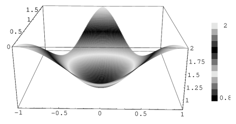
Figure 1: (a) The three-point correlator (20), (21) for single-field slow-roll inflation, multiplied by $k_{1}^{3}k_{2}^{3}k_{3}^{3}/((k_{1}^{2}+k_{2}^{2}+k_{3}^{2})/2)^{3/2}[(\kappa^{4}/16)(H^{4}/{\tilde{\epsilon}}^{2})(2{\tilde{\epsilon}}+{\tilde{\eta}})]^{-1}$, plotted to show its dependence on the relative size of the three momenta. (b) An explanation of the triangular domain used, defined in (23).

However, since we have obtained the full momentum dependence, it is interesting to go beyond this specific limit. Actually the three-point correlator does not depend on the three full vectors ${\mathbf{k}}_{1},{\mathbf{k}}_{2},{\mathbf{k}}_{3}$, but only on three scalar quantities, which can be taken to be the three lengths $k_{1},k_{2},k_{3}$ (physically this corresponds to statistical isotropy). We can redefine variables to get the overall magnitude $k\equiv k_{1}+k_{2}+k_{3}$ and two ratios $\gamma$ and $\beta$,

$$\gamma\equiv 2\,\frac{k_{2}-k_{3}}{k},\qquad\beta\equiv-\sqrt{3}\,\frac{k_{1}-k_{2}-k_{3}}{k},$$ (23)

which means that

$$k_{1}=\frac{k}{2}\left(1-\frac{\beta}{\sqrt{3}}\right),\qquad k_{2,3}=\frac{k}{4}\left(1\pm\gamma+\frac{\beta}{\sqrt{3}}\right).$$ (24)

In addition, because ${\mathbf{k}}_{1}+{\mathbf{k}}_{2}+{\mathbf{k}}_{3}={\mathbf{0}}$, one can use relations like $|{\mathbf{k}}_{1}+{\mathbf{k}}_{2}|^{2}=k_{3}^{2}$ and ${\mathbf{k}}_{1}\cdot{\mathbf{k}}_{2}=(k_{3}^{2}-k_{1}^{2}-k_{2}^{2})/2$. The domain of $\gamma$ and $\beta$ is an equilateral triangle as shown in figure 1. The vertices of the triangle correspond to one of the three momenta being zero (the limit for (22)), while the sides correspond to one of the momenta being equal to half the total sum ($k/2$). From its vertex to the opposite side $k_{s}$ grows linearly. Plotting the three-point correlator in such a way demonstrates its symmetry most clearly, as shown in figure 1. The three-point correlator in that plot has been multiplied by $k_{1}^{3}k_{2}^{3}k_{3}^{3}/((k_{1}^{2}+k_{2}^{2}+k_{3}^{2})/2)^{3/2}$ to remove the overall $k$ magnitude, and the factor of $(\kappa^{4}/16)(H^{4}/{\tilde{\epsilon}}^{2})(2{\tilde{\epsilon}}+{\tilde{\eta}})$ has also been omitted (assuming that the momentum dependence of $H_{\mathcal{H}}$ and the slow-roll parameters can be neglected). There is some dependence on the relative magnitude of the momenta, but it is only a variation of order unity for the single-field case.

We finish this section by remarking on the decaying mode. Even though it disappears very quickly after horizon crossing, one might think that including it could improve the accuracy of the result, since the window function does operate near horizon crossing. When taking into account the decaying mode, ${\mathcal{J}}_{i}$ is no longer zero, and we have to include the $\theta_{i}$ equation. Fortunately we can still solve this system analytically. In the limit of $R\rightarrow 0$ we find that $\zeta^{(1)}$ is unchanged, while $\zeta^{(2)}$ picks up an additional term: $(2{\tilde{\epsilon}}_{{\mathcal{H}}^{\prime}}+{\tilde{\eta}}_{{\mathcal{H}}^{\prime}})k^{2}/(k^{2}+{k^{\prime}}^{2})\,\alpha({\mathbf{k}}^{\prime})$ in (Simple route to non-Gaussianity in inflation) is replaced by

$$(2{\tilde{\epsilon}}_{{\mathcal{H}}^{\prime}}+{\tilde{\eta}}_{{\mathcal{H}}^{\prime}})\frac{k^{2}}{k^{2}+{k^{\prime}}^{2}}\,\alpha({\mathbf{k}}^{\prime})+3\sqrt{\frac{\pi}{2}}\frac{1}{c^{3}}\frac{k^{2}{k^{\prime}}^{3}}{(k^{2}+{k^{\prime}}^{2})^{\frac{5}{2}}}\,\mathrm{i}\alpha({\mathbf{k}}^{\prime}).$$ (25)

We see that the additional term is not suppressed by slow-roll factors, but by a factor $1/c^{3}$ and thus depends on the smoothing length. However, once we compute the three-point correlator, we find that the additional term drops out exactly, because of the relative phase factor $\mathrm{i}$. Hence for the final result dropping the decaying modes is not an approximation.

Discussion — We have illustrated a new method for calculating non-linearity in inflation, which was introduced in gp2 ; formalism , with an explicit calculation in the single-field case. Analytic resuls were derived to second order in a perturbative expansion and to leading order in slow roll. We derived a general expression for the three-point correlator of the curvature perturbation in Fourier space (the bispectrum). In the limit of one of the momenta being much smaller than the other two, the expression reduces to a simple result: the scalar spectral index times the square of the power spectrum. This agrees with previous results in the literature but it was derived in a much simpler way. In particular, it agrees exactly with the tree-level action calculation of Maldacena mald . We also demonstrated that the decaying mode makes no contribution to the three-point correlator at this order.

We introduced convenient variables to plot the full momentum dependence of the three-point correlator. In mald the three-point correlator is also given in the limit of all three momenta being equal, which corresponds with the centre of the triangle in figure 1. Although similar in magnitude, our expression differs in the exact value there. This is probably due to our use of a linear stochastic term to emulate the effects of sub-horizon perturbations, which does not fully include cubic interactions around horizon crossing. As is shown in mf , the terms causing this discrepancy are subdominant in the multiple-field case.

For the single-field case non-Gaussianity is suppressed by slow-roll factors, and hence unobservable for models that satisfy the CMB constraints. However, this is not necessarily the case for multiple-field inflation models uzan ; mf , where the non-Gaussianity can be large. The main strength of our method, apart from being simple, is that it is easily applicable to general multiple-field inflation; indeed, the basic equations for the multiple-field case were already presented in gp2 ; formalism . The formalism is also well-suited for numerical implementation; no slow-roll approximation is needed, and the end result is a real-space realisation, which contains more information than just the $N$-point correlator. Results from our numerical implementation of the formalism will be presented in another paper. We believe that the simplicity of this formalism, its general applicability, and its suitability for numerical simulations make it very useful for future studies of non-Gaussianity from inflation.

References

- (1) J. Lesgourgues, D. Polarski, and A.A. Starobinsky, Nucl. Phys. B497, 479 (1997) [gr-qc/9611019]; A. Gangui, J. Martin, and M. Sakellariadou, Phys. Rev. D66, 083502 (2002).
- (2) A.R. Liddle and D.H. Lyth, Cosmological Inflation and Large-Scale Structure (Cambridge University Press, Cambridge, 2000).
- (3) E. Komatsu, Ph.D. thesis, Tohoku University, 2001 [astro-ph/0206039].
- (4) D.S. Salopek and J.R. Bond, Phys. Rev. D43, 1005 (1991); A. Gangui, F. Lucchin, S. Matarrese, and S. Mollerach, Astrophys. J. 430, 447 (1994) [astro-ph/9312033]; I. Yi and E.T. Vishniac, Astrophys. J. Suppl. 86, 333 (1993).
- (5) V. Acquaviva, N. Bartolo, S. Matarrese, and A. Riotto, Nucl. Phys. B667, 119 (2003) [astro-ph/0209156].
- (6) H. Noh and J.-C. Hwang, Phys. Rev. D69, 104011 (2004) [astro-ph/0305123].
- (7) N. Bartolo, E. Komatsu, S. Matarrese, and A. Riotto, Phys. Rep. 402, 103 (2004) [astro-ph/0406398].
- (8) J. Maldacena, JHEP 0305, 013 (2003) [astro-ph/0210603].
- (9) G.I. Rigopoulos and E.P.S. Shellard, JCAP 0510, 006 (2005) [astro-ph/0405185].
- (10) G.I. Rigopoulos, E.P.S. Shellard, and B.J.W. van Tent, astro-ph/0504508.
- (11) G.I. Rigopoulos, E.P.S. Shellard, and B.J.W. van Tent, astro-ph/0506704.
- (12) A.A. Starobinsky, in Field Theory, Quantum Gravity and Strings, edited by H.J. De Vega and N. Sanchez (Springer, Berlin, 1986), p.107 ; K. Nakao, Y. Nambu, and M. Sasaki, Progr. Theor. Phys. 80, 1041 (1988); H.E. Kandrup, Phys. Rev. D39, 2245 (1989); D.S. Salopek and J.R. Bond, Phys. Rev. D43, 1005 (1991); J.M. Stewart, Class. Quant. Grav. 8, 909 (1991); H. Casini, R. Montemayor, and P. Sisterna, Phys. Rev. D59, 063512 (1999) [gr-qc/9811083]; S. Winitzki and A. Vilenkin, Phys. Rev. D61, 084008 (2000) [gr-qc/9911029]; N. Afshordi and R.H. Brandenberger, Phys. Rev. D63, 123505 (2001) [gr-qc/0011075]; S. Matarrese, M.A. Musso, and A. Riotto, JCAP 0405, 008 (2004) [hep-th/0311059]; G. Geshnizjani and N. Afshordi, JCAP 0501, 011 (2005) [gr-qc/0405117].
- (13) A.H. Guth and S.-Y. Pi, Phys. Rev. D32, 1899 (1985); A. Albrecht, P. Ferreira, M. Joyce, and T. Prokopec, Phys. Rev. D50, 4807 (1994) [astro-ph/9303001]; D. Polarski and A.A. Starobinsky, Class. Quantum Grav. 13 377 (1996) [gr-qc/9504030].
- (14) G.L. Comer, N. Deruelle, D. Langlois, and J. Parry, Phys. Rev. D49, 2759 (1994); N. Deruelle and D. Langlois, Phys. Rev. D52, 2007 (1995) [gr-qc/9411040] and references therein; J. Parry, D.S. Salopek, and J.M. Stewart, Phys. Rev. D49, 2872 (1994) [gr-qc/9310020]; I.M. Khalatnikov, A.Yu. Kamenshchik, and A.A. Starobinsky, Class. Quantum Grav. 19, 3845 (2002) [gr-qc/0204045].
- (15) M. Giovannini, JCAP 0509, 009 (2005) [astro-ph/0506715].
- (16) G.I. Rigopoulos and E.P.S. Shellard, Phys. Rev. D68, 123518 (2003) [astro-ph/0306620].
- (17) V.F. Mukhanov, H.A. Feldman, and R.H. Brandenberger, Phys. Rep. 215, 203 (1992).
- (18) S. Groot Nibbelink and B.J.W. van Tent, Class. Quantum Grav. 19, 613 (2002) [hep-ph/0107272].
- (19) F. Bernardeau and J.-P. Uzan, Phys. Rev. D66, 103506 (2002) [hep-ph/0207295]; D67, 121301 (2003) [astro-ph/0209330].