Nonlocal String Tachyon as a Model for Cosmological Dark Energy

Abstract

There are many different phenomenological models describing the cosmological dark energy and accelerating Universe by choosing adjustable functions. In this paper we consider a specific model of scalar tachyon field which is derived from the NSR string field theory and study its cosmological applications. We find that in the effective field theory approximation the equation of state parameter $w<-1$, i.e. one has a phantom Universe. It is shown that due to nonlocal effects there is no quantum instability that the usual phantom models suffer from. Moreover due to a flip effect of the potential the Universe does not enter to a future singularity.

1 Introduction

It was suggested by Ia Supernova observations that the Universe is presently accelerating[1, 2]. The basic sets of experiments now includes also the Cosmic Microwave Background (CMB) anisotropies, X-ray data from galaxy clusters, large scale structure and age estimates of global clusters, for a review see [3, 4, 5]. It is believed that a new particle and/or gravitational physics is required to explain the acceleration of the expansion of the Universe. The observations suggest that the bulk of energy density in the Universe is gravitationally repulsive and appears like an unknown form of energy (dark energy) with negative pressure. It is believed that 2/3 of the total density of the universe is in a form of dark energy.

There exist many different models of dark energy. It is convenient to describe them by using the equation of state parameter $w=p/\rho$, where $p$ is a pressure and $\rho$ is the energy density. The analysis of the current observation data shows that $w$ lies in the range $-1.61<w<-0.78$ [6, 3, 7].

A list of dark energy models includes (see [4]-[23] and refs. therein)

• $w=-1$: the cosmological constant;

• $w=const\neq-1$: the cosmic strings, domain walls, etc.;

• $w\neq const$: quintessence scalar field, chaplygin gas, k-essence, Dirac-Born-Infeld(DBI) action, braneworlds, etc.;

• $w<-1$: phantom models.

The most challenging for theoretical physics would be the case $w<-1$ [12]-[17] (see [19, 5, 20] for reviews). In this case the weak energy condition ($\rho>0,\rho+p>0$) is violated and some strange phenomena as negative entropy and temperature appear. In many models the phantom Universe in finite time ends up in the singularity called the Big Rip [14]).

In this paper we consider string field theories nonlocal tachyon where the condition $w<-1$ is realized. We show that due to a peculiar properties of nonlocal tachyon dynamics we can get a phantom universe without problems with unstability. A nonlocal dynamics for the tachyon field is obtained by truncation of the covariant string field equations. We study a nonlocal dynamics of a string tachyon in the cosmological Friedmann metric. The string theory that we have in mind is the NSR string theory compactified on a six dimensional compact manifold. Moreover we assume that all moduli are frozen and unstable non-BPS brane extends along the three large spatial dimensions. The tension of the 3-dimensional non-BPS brane acts as the 4-dimensional universe cosmological constant and the tachyon dynamics describes a deviation from a pure cosmological constant regime.

A presence of tachyons was considered as a main drawback of corresponding strings theory. Bosonic string has a tachyon and its absence in superstrings was a main motivation to introduce superstrings. However few years ego tachyon has found an application in the context of brane scenarios. The open bosonic string and GSO $-$ NSR string tachyons were used to describe D-brane decays. According to the Sen conjecture in the perturbative vacuum there are instable branes filling space-time and all these branes disappear in the true vacuum (for review see [24],[25]). Rolling tachyon solutions describe transitions from perturbative vacuum to non-perturbative one.

Here we use the covariant open string field theory(SFT) approach [24] to tachyon dynamics (about the effective DBI approach to tachyon dynamics see [26],[27],[25] and refs. therein). A crucial feature of the rolling tachyon solution for non-BPS brane [30] is that it interpolates between two non-perturbative vacua with the same energy. We argue that at large time the dynamics is governed by an effective action that contains a ghost kinetic term, in spite of absence of ghosts in the nonlocal action. We emphasize that the ghost here is a result of an approximation to the exact nonlocal action. There is no ghost in the nonlocal action. So we get a phantom universe as an approximation to the true nonlocal dynamics. This is the reason why there are no pathologies in this scenario with the thermodynamical instabilities.

The rolling tachyon solution passes the perturbative vacuum with non-zero velocity. Therefore, to reach the true vacuum starting from the perturbative one we have to supply the tachyon with a large enough initial velocity . This is a rather non-standard situation from the local field theory point of view, where one does not have to push strongly the tachyon to make it reach the true vacuum, it is need just an infinitesimal small perturbation. This effect occurs due to the presence of derivative terms in the interaction. These terms may be studied in an effective action approximation, which corresponds to keeping only few terms of an expansion of an nonlocal operator. We note that to reach the nonperturbative vacuum one has to add to the action a brane tension which is larger that is required by the Sen hypothesis. This large brane tension can be interpreted as an effect of the closed string excitations.

We find that in the effective field theory approximation the equation of state parameter $w<-1$, i.e. one has a phantom Universe. In the DBI approach the equation of state parameter interpolates between -1 at early time and 0 at a later time. Within application of the DBI action to cosmology there are problems with large density perturbations, reheating and caustics formation [28, 29].

The paper is organizes as follows. In Sect. 2.1. the nonlocal tachyon action is written in the Friedmann background. In Sect. 2.2 we shortly remind a construction of the rolling tachyon solution for non-BPS brane [30]. In Sect. 2.3 we study the tachyon dynamics in the Friedmann metric in the effective action approximation. In this approximation one gets $w<-1$. In Sect. 2.4 we show that to reach a nonperturbative vacuum one has to add to the action a brane tension which is larger that is required by the Sen hypothesis. In Sect. 3 we show the stability of the nonlocal tachyon model in the true vacuum.

2 Non-BPS tachyon in Friedmann space-time

2.1 General set up

We consider a non-BPS tachyon leaving on 3-brane and interacting with gravity with the following action

$$S=\frac{M_{p}^{2}}{2}\int\sqrt{-g}d^{4}x\,R+S_{tach}\ .$$ (2.1)

where

$$S_{tach}=\int\;\sqrt{-g}d^{4}x\left(-\frac{q^{2}}{2}g^{\mu\nu}\partial_{\mu}\phi\partial_{\nu}\phi+\frac{1}{2}\phi^{2}-\frac{1}{4}\Phi^{4}\right),$$ (2.2)

$\Phi=\exp(\frac{1}{2}\Box_{g})\phi$, $\Box_{g}=\frac{1}{\sqrt{-g}}\partial_{\mu}\sqrt{-g}g^{\mu\nu}\partial_{\nu}$, $q^{2}=const<1$. Here we assume that all constants are absorbed into $M^{2}_{p}$. The action (2.2) generalizes the non-BPS tachyon action obtained from low level truncated SFT to the case of a non-flat metric [30].

On space homogeneous configurations in the Friedmann metric

$$ds^{2}=-dt^{2}+a^{2}(t)(dr^{2}+r^{2}(d\theta^{2}+\sin^{2}\theta d\phi^{2}))$$ (2.3)

the action (2.2) takes the form

$$S_{tach}[\phi]=\int\;\sqrt{-g}dt\left[\frac{1}{2}\phi^{2}(t)+\frac{q^{2}}{2}\dot{\phi}(t)^{2}-\frac{1}{4}\Phi^{4}(t)\right],$$ (2.4)

where $\Phi=\exp(\frac{1}{2}{\cal D})\phi$, ${\cal D}=-\partial_{t}^{2}-3H(t)\partial_{t}$ and $H(t)=\dot{a}/a$, $\dot{a}=\partial_{t}a$. The Einstein equations have the form

$$3H^{2} = \frac{1}{M^{2}_{p}}~{}~{}\rho$$ (2.5)

$$H^{2}+2\ddot{a}/a = -\frac{1}{M^{2}_{p}}~{}~{}p$$ (2.6)

with the energy and pressure densities are given by [30]

$$\rho=\frac{q^{2}}{2}(e^{-\frac{1}{2}{\cal D}}\dot{\Phi})^{2}-\frac{1}{2}(e^{-\frac{1}{2}{\cal D}}\Phi)^{2}+\frac{1}{4}\Phi^{4}+{\cal E}_{1}+{\cal E}_{2}]$$ (2.7)

$$p=\frac{q^{2}}{2}(e^{-\frac{1}{2}{\cal D}}\dot{\Phi})^{2}+\frac{1}{2}(e^{-\frac{1}{2}{\cal D}}\Phi)^{2}-\frac{1}{4}\Phi^{4}-{\cal E}_{1}+{\cal E}_{2}.$$ (2.8)

where

$${\cal E}_{1}=-\frac{1}{2}\int_{0}^{1}d\rho(e^{\frac{1}{2}\tau{\cal D}}\Phi^{3}){\cal D}e^{-\frac{1}{2}\tau{\cal D}}\Phi$$ (2.9)

$${\cal E}_{2}=-\frac{1}{2}\int_{0}^{1}d\tau(\partial_{t}e^{\frac{1}{2}\tau{\cal D}}\Phi^{3})\partial_{t}e^{-\frac{1}{2}\tau{\cal D}}\Phi$$ (2.10)

Equation of motion for the scalar field is

$$\left(q^{2}{\cal D}+1\right)e^{-{\cal D}}\Phi=\Phi^{3}.$$ (2.11)

2.2 Rolling solution in flat space-time

Taking $H=0$ in (2.11) we get the following equation in the flat space

$$\left(-q^{2}\partial_{t}^{2}+1\right)e^{\partial^{2}}\Phi=\Phi^{3}.$$ (2.12)

This equation contains infinite number of time derivatives, and actually can be written in the integral form. It has been shown numerically that for $q^{2}$ small enough there is a solution that interpolates between non trivial vacua $\Phi(\pm\infty)=\pm 1$ and $\Phi(0)=0$ [32]. One can get an approximation to this solution expanding the exponent in (2.12) in powers of derivatives and keeping only the second derivatives,

$$\left((1-q^{2})\partial_{t}^{2}+1\right)\Phi(t)=\Phi^{3}(t).$$ (2.13)

This equation describes a particle moving in the potential $V=\frac{(\Phi^{2}-1)^{2}}{4(q^{2}-1)}+const$. For $q^{2}<1$ the factor $q^{2}-1$ flips the potential, Fig.1.

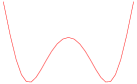
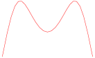
$a)~{}~{}~{}~{}~{}~{}~{}$ $~{}~{}b)$

Figure 1: Flip of the potential for $q^{2}<1$

Equation (2.13) for $q^{2}<1$ has the kink solution $\Phi_{kink}$. Kink interpolates between two vacua during infinitely long time and it is represented in Fig.2a by a thin line.

$a~{}~{}~{}$ $b~{}~{}~{}~{}~{}$ $c$

Figure 2: a) kink $\Phi_{kink}(t)$ (thin line) and $\Phi_{0}(t)$ (think line); b) $\Phi(t)$ for $q^{2}=0.96$;      c) oscillations of $\Phi(t)$ with decreasing amplitudes around $\Phi_{0}$

Equation (2.12) for $q=0$ (the p-adic string equation of motion for $p=3$) also has a interpolating solution [33, 34, 32]. We denote it $\Phi_{0}(t)$ and plot it in Fig. 2a by think line. Note that the function $\Phi_{0}(t)$ is monotonic. From Fig.2a we see that $\Phi_{kink}$ and $\Phi_{0}$ have different profiles, but this difference is not too big for large times. There is an essential difference at small time. $\Phi_{kink}$ has the finite first derivative at $t=0$, meanwhile the first derivative of $\Phi_{0}(t)$ becomes infinite at $t=0$. Note, that the derivative of the initial scalar field $\phi$ related with $\Phi$ via $\phi=e^{-\frac{1}{2}{\cal D}}\Phi$ is finite at $t=0$. Therefore, higher derivatives in (2.12) change the profile of $\Phi_{kink}(t)$ only at small time and do not change the asymptotic behavior at large time.

Note, that small $q^{2}$ also does not change too much a profile of a solution to (2.12) interpolating between two vacua. This solution is plotted in Fig.2b. The profile of this solution is not a monotonic function. It can be presented as $\Phi(t)=\Phi_{0}(t)+\phi(t)$, where $\phi(t)$ describes oscillations around $\Phi_{0}$ with decreasing amplitude. These oscillations are presented in Fig.2c.

2.3 Approximate solution of system of equations for Non-BPS tachyon in Friedmann space-time

Motivated by the flat case we make in (2.11) an approximation

$$\exp(\partial_{t}^{2}+3H(t)\partial_{t})\Phi\approx(~{}1+\partial_{t}^{2}+3H(t)\partial_{t}~{})~{}\Phi$$ (2.14)

and keep only terms linear on $(1+\partial_{t}^{2}+3H(t)\partial_{t}~{})$. It is evident that this equation can be obtained from the action

$$S^{\prime}_{scalar}=\int\sqrt{-g}d^{4}x\,\left(\frac{1-q^{2}}{2}g^{\mu\nu}\partial_{\mu}\Phi\partial_{\nu}\Phi-V(\Phi)\right)\ .$$ (2.15)

We see that for $q^{2}<1$ we get the ghost sign in front of the kinetic terms. Assuming that $q^{2}<1$ we take for simplicity in the following formula $q^{2}=0$ ($q^{2}<1$ can be achieved just by rescaling of time). The corresponding Einstein equations have the form (2.7), (2.8) with

$$\rho = -\frac{1}{2}\dot{\Phi}^{2}+V(\Phi),$$ (2.16)

$$p = -\frac{1}{2}\dot{\Phi}^{2}-V(\Phi)$$ (2.17)

and the equation for $\Phi$ field read

$$\ddot{\Phi}+3H\dot{\Phi}=V^{\prime}_{\Phi}$$ (2.18)

Excluding $H$ from (2.7) and (2.18) one gets the following equation

$$\ddot{\Phi}+\frac{1}{M_{p}}\dot{\Phi}~{}\sqrt{3[-\frac{1}{2}\dot{\Phi}^{2}+V(\Phi)]}-V^{\prime}_{\Phi}=0$$ (2.19)

We see that an equation similar to the usual scalar field equation in the Friedmann metric. There are only two different signs, one in front of the kinetic energy in the square root, and the second in front of the derivative of the potential. It is evident that solutions of this equation in the slow-roll regime are the same as in the usual case with ”-” potential. However there are differences in the fast roll regime. The equation state parameter $w$

$$w=\frac{p}{\rho}=\frac{\frac{1}{2}\dot{\Phi}^{2}+V(\Phi)}{\frac{1}{2}\dot{\Phi}^{2}-V(\Phi)}$$ (2.20)

is always less then -1, since $w$ can be represented also as

$$w=-\frac{3H^{2}+2\dot{H}}{3H^{2}}=-1-\frac{2}{3}\frac{\dot{H}}{H^{2}}$$ (2.21)

and from the equation of motions follows

$$\dot{H}=\frac{1}{2M^{2}_{p}}\dot{\Phi}^{2},$$ (2.22)

i.e. $\dot{H}$ is positive.

2.4 Numerical solutions

Let us examine numerically solution of the system of equations (2.16) and (2.18) for the potential

$$V(\Phi)=\frac{1}{4}\left(\Phi^{2}-1\right)^{2}$$ (2.23)

$a~{}$ $b$ $c$ $d$

Figure 3: a) Plot of $\Phi=\Phi(t)$ with $\Phi(0)=-1$ and $\dot{\Phi}\simeq 0$; b) plot of $H=H(t)$; plot of $w=w(t)$ for c) $0<t<8$ and d) for $8<t<15$

There are two independent initial conditions for $\Phi(0)$ and $\dot{\Phi}(0)$. If the initial position $\Phi(0)$ is on the the top of the hill (for the flip potential, Fig.1.b), $\Phi(0)=-1$, and the initial velocity is very small $\dot{\Phi}(0)\simeq 0$ (this corresponds to $H(0)\simeq 0$) then after some time $\Phi$ reaches the largest position and goes back to the bottom, and then performs few oscillations and stops at the bottom. The final value of $H$ is $1/2\sqrt{3}$. The evolutions of the scalar field and log-derivative of the scale factor are represented in Fig.3.a and Fig.3.b. The evolution of the state equation parameter $w$ is plotted in Fig.3c,d. It starts from -1, becomes a very big negative number when the field passes the bottom of the flip potential Fig.3c and goes with small fluctuations to $-1$ at large times. Fig.3.d shows that these fluctuations do not exceed $-1$.

To reach the top of the hill $\Phi=1$ one has to increase the velocity, but since there is a restriction on the initial velocity $\dot{\Phi}(0)^{2}\leq 2V(0)$, (the initial energy should be positive), one has to add a positive constant $V_{0}$ to the potential to be able to increase the initial velocity.

For large $M_{p}$ and a suitable $V_{0}$ there is a solution that starts from the top of one hill with a non-zero velocity and reach the top of other hill during an infinite time, Fig.4. In this case during the initial stages of evolution the field is near the top of the hill, $\Phi=-1$ and the acceleration is small. At later times the field begins to evolve more rapidly towards the local minimum of the flip potential and the equation state parameter $w$ becomes rather big. Finally, in very late time the field comes closed to the top of other hill, $\Phi=1$

$$\Phi=1-Ae^{-\alpha t},$$ (2.24)

where $A$ is an arbitrary constant, $\alpha=(\frac{\sqrt{3V_{0}}}{M_{p}}+\sqrt{\frac{3V_{0}}{M^{2}_{p}}+8})/2$ and a period of $w\simeq-1$, $w<-1$ begins. This period is infinitely long because the flip potential has the maximum at $\Phi=1$.

           

Figure 4: Plots of $\phi(t)$, $H(t)$ and $w(t)$ for $\phi(0)=-1,\dot{\phi}(0)=0.1,V_{0}=0.02$

3 Stability

In this section we show that fluctuations of the scalar field around the true vacua are stable for suitable $q^{2}$, namely we show that the Euclidian action is positive defined.

For the usual Goldstone model in the flat space-time (2.23) fluctuations around one of minima $\Phi_{0}=\pm 1$ correspond to massive excitations. In our case due to nonlocal factors in the interaction we get a different picture. Depending on parameter $q^{2}$ we get two excitations with different positive square mass or do not get any excitation at all.

Indeed, for fluctuations around $\Phi_{0}=1$

$$\Phi=\Phi_{0}+\delta\Phi$$ (3.25)

we get the quadratic part of the action

$$S_{0}=\int\delta\Phi\left((q^{2}\Box+1)e^{-\Box}-3\right)\delta\Phi dx$$ (3.26)

To get the particle spectrum we are looking for solutions of the equation

$$-q^{2}m^{2}-1+3e^{m^{2}}=0$$ (3.27)

with $=-k_{0}^{2}+\vec{k}^{2}\equiv k^{2}=-m^{2}<0$. To find solutions of this equation we plot in Fig. 5 the function

$$f(x)=-q^{2}x-1+3e^{x}$$ (3.28)

and find its zeros.

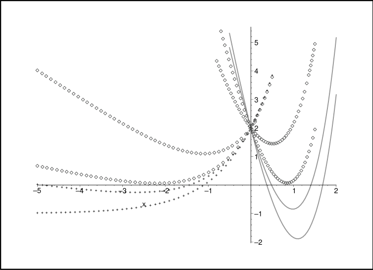
Figure 5: Plots of function $f(x)=-q^{2}x-1+3e^{2x}$ for different values of $q^{2}$$:q^{2}<q^{2}_{cr1}$ (cross lines), $q^{2}_{cr1}<q^{2}<q^{2}_{cr2}$ (diamond lines), $q^{2}>q^{2}_{cr2}$ (solid lines)$;q^{2}_{cr1}\simeq 0.33$, $q^{2}_{cr2}\simeq 7$

We see that for $q^{2}<q^{2}_{cr2}$ this curve has no positive zeros. For $q^{2}>q^{2}_{cr2}$ there are two zeros, $f(m^{2}_{i})=0$ with $m_{i}^{2}>0,~{}~{}~{}i=1,2$. Therefore there are no massive excitations for $q^{2}<q^{2}_{cr2}$, and there are two massive particles for $q^{2}>q^{2}_{cr2}$. There is one massive particle for $q^{2}_{cr}$.

For $q^{2}<q_{cr1}$ the function $f(x)$ has also zero for a negative argument (see ”cross-lines” on Fig.5) that corresponds to an appearance of tachyons.

Let us note that our propagator around new vacuum is non-standard one. If we expand $\exp(-\Box)$ in power of derivatives keeping only the first order terms on $\Box$ we get

$$S_{0}\approx-\int\delta\Phi(k)\left((q^{2}-1)k^{2}+2\right)\delta\Phi(-k)dk$$ (3.29)

and we see that the case $q^{2}<1$ looks like as if the ghosts are appearing. In particular, this means that if we performing the Euclidean rotations $k^{2}=-\omega^{2}+\vec{k}\to k^{2}_{E}$, then our approximated Euclidean propagator $\left((q^{2}-1)k_{E}^{2}+2\right)$ for $q^{2}<1$ it is not positively defined. However, the full propagator that one gets from $S_{0}$ after the Euclidean rotations

$$S_{0}=-\int\delta\Phi(k)\left((q^{2}k_{E}^{2}-1)e^{k_{E}^{2}}+3\right)\delta\Phi(-k)dk$$ (3.30)

is positive defined for $q^{2}_{cr1}<q^{2}<q^{2}_{cr2}$. Indeed,

$$\left((q^{2}k_{E}^{2}-1)e^{k_{E}^{2}}+3\right)=f(-k_{E}^{2})e^{k_{E}^{2}}$$ (3.31)

and we see form Fig.5 that the function f(x) for negative arguments is positive for all negative arguments (positive $k^{2}_{E}$) if $q^{2}>q^{2}_{cr1}$. Therefore, we see that the inverse propagator is strictly positive for $q_{cr2}^{2}>q^{2}>q_{cr1}^{2}$. It is interesting to note that for $q^{2}=0$ the inverse propagator $f(-k_{E}^{2})e^{2k_{E}^{2}}$ is not positive.

4 Conclusion

We have studied the evolution of open GSO $-$ NSR string tachyon in the Friedmann space-time. The corresponding solution in the flat space-time is known as a rolling tachyon and it describes the decay of the space filling D3 brane corresponding to the unstable perturbative vacuum to the local stable vacuum. We have performed calculations under the following approximations and assumptions:

• the level truncation and an approximation of a slow varying axillary field;

• a direct generalization of the tachyon nonlocal action to the Friedmann space-time;

• an effective local action approximation.

We have found that in the effective field theory approximation the equation of state parameter $w<-1$, i.e. one has a phantom Universe, but there is no problem with quantum instability without this approximation. We have found that to reach the nonperturbative vacuum one has to add to the action a brane tension which is larger that is required by the Sen hypothesis. This large brane tension can be interpreted as an effect of the closed string excitations.

It would be interesting to try to find an analog of this solution to a full SFT theory (without level truncation), in particular with a framework of Vacuum String Field Theory. VSFT is a version of usual SFT that is supposed to describe the theory at the minimum of the tachyon potential. Corresponding solutions for bosonic VSFT have been found recently in [35]. It would be also interesting to see if one has to shift the tension of D-brane to get a rolling solution in the Friedmann metric.

 

Acknowledgements

I would like to thank L. Bonora, B. Dragovich, A. Koshelev, S. Mukhanov, S. Vernov and I. Volovich for useful discussions. This work is supported in part by RFBR grant 02-01-00695 and INTAS grant 03-51-6346.

References

- [1] S.J. Perlmutter et al., 1999 Astroph. J. 517 565, Measurements of Omega and Lambda from 42 High-Redshift Supernovae, astro-ph/9812133
- [2] A. Riess et al., 1998 Astron. J. 116 1009, Observational Evidence from Supernovae for an Accelerating Universe and a Cosmological Constant, astro-ph/9805201
- [3] D. N. Spergel et al., 2003 Astroph. J. Suppl. 148 175, First Year Wilkinson Microwave Anisotropy Probe (WMAP) Observations: Determination of Cosmological Parameters, astro-ph/0302209
- [4] V. Sahni and A. A.Starobinsky, Int. J. Mod. Phys. D9 (2000) 373, The Case for a Positive Cosmological Lambda-term, astro-ph/9904398.
- [5] V. Sahni, Dark Matter and Dark Energy, astro-ph/0403324
- [6] R.A.Knop et al., New constraints on , , and w from an independent set of eleven high - redshift supernovae observed with HST, astro-ph/0309368.
- [7] M. Tegmark al., Astroph. J. 606 (2004) 702-740, The 3-d power spectrum of galaxies from the SDSS, astro-ph/0310723
- [8] C. Armendariz-Picon, V. Mukhanov and P. J.Steinhardt, Phys. Rev. Lett. 85 (2000) 4438, A Dynamical Solution to the Problem of a Small Cosmological Constant and Late-time Cosmic Acceleration, astro-ph/0004134
- [9] Deffayet C, Dvali G and Gabadadze G, Phys. Rev. D 65 (2002) 044023, Accelerated Universe from Gravity Leaking to Extra Dimensions, astro-ph/0105068
- [10] U. Alam, V. Sahni and A. A. Starobinsky, The case for dynamical dark energy revisited, astro-ph/0403687
- [11] T.Padmanabhan, Accelerated expansion of the universe driven by tachyonic matter , Phys.Rev. D66 (2002) 021301, hep-th/0204150; T. Padmanabhan, T. Roy Choudhury Can the clustered dark matter and the smooth dark energy arise from the same scalar field ? , hep-th/0205055, Phys.Rev. D66 (2002) 081301;
- [12] Caldwell R R, Phys. Lett. B 545 (2002) 23, A Phantom Menace? Cosmological consequences of a dark energy component with super-negative equation of state, astro-ph/9908168
- [13] McInnes B, JHEP 0208 (2002) 029, The dS/CFT Correspondence and the Big Smash, hep-th/0112066
- [14] Caldwell R R, Kamionkowski M and Weinberg N N, Phys. Rev. Lett. 91 (2003) 071301, Phantom Energy and Cosmic Doomsday, astro-ph/0302506
- [15] V.K. Onemli, R.P. Woodard, Super-Acceleration from Massless, Minimally Coupled , Class.Quant.Grav. 19 (2002) 4607, gr-qc/0204065; V. K. Onemli, R. P. Woodard Quantum effects can render w¡-1 on cosmological scales, Phys.Rev. D70 (2004) 107301, gr-qc/0406098
- [16] Carroll S M, Hoffman M and Trodden M, Phys. Rev. D 68 (2003) 023509, Can the dark energy equation-of-state parameter w be less than -1? , astro-ph/0301273
- [17] Melchiorri A, Mersini L, Odman C J and Trodden M, Phys. Rev. D 68 (2003) 043509, The State of the Dark Energy Equation of State, astro-ph/0211522
- [18] J. Krakochvil, A.Linde, E.Linder and M.Shmakova, Testing the Cosmological Constant as a Candidate for Dark Energy, astro-ph/0312183
- [19] P. Frampton, Dark energy - a pedagogic review, hep-th/0409166
- [20] T.Padmanabhan, Cosmological Constant - the Weight of the Vacuum, Phys.Rept. 380 (2003) 235-320, hep-th/0212290
- [21] Bo Feng, Xiulian Wang, Xinmin Zhang, Dark Energy Constraints from the Cosmic Age and Supernova, astro-ph/0404224; Bo Feng, Mingzhe Li, Yun-Song Piao, Xinmin Zhang, Oscillating Quintom and the Recurrent Universe, astro-ph/0407432
- [22] S. Nojiri and S.Odintsov, The final state and thermodynamics of dark energy universe, hep-th/0408170
- [23] W.Fang, H.Q.Lu, Z.G. Huang and K.F..Zhang, Phantom Cosmology with Born-Infeld Type Scalar Field, hep-th/0409080
- [24] K. Ohmori, A Review on Tachyon Condensation in Open String Field Theories, hep-th/0102085; I.Ya. Aref’eva, D.M. Belov, A.A. Giryavets, A.S. Koshelev, P.B. Medvedev, Noncommutative Field Theories and (Super)String Field Theories, hep-th/0111208; W.Taylor, Lectures on D-branes, tachyon condensation and string field theory, hep-th/0301094.
- [25] A. Sen, Tachyon Dynamics in Open String Theory, hep-th/0410103.
- [26] A. Sen, JHEP 0204, 048 (2002), Rolling Tachyon, hep-th/0203211; A. Sen, JHEP 0207, 065 (2002), Tachyon Matter, hep-th/0203265;
- [27] G.W. Gibbons, Thoughts on Tachyon Cosmology, Class.Quant.Grav. 20 (2003) S321-S346, hep-th/0301117.
- [28] Gary N. Felder, Lev Kofman, Alexei Starobinsky, Caustics in tachyon matter and other Born-Infeld scalars. JHEP 0209:026,2002. hep-th/0208019;
- [29] Andrei V. Frolov, Lev Kofman, Alexei A. Starobinsky, Prospects and problems of tachyon matter cosmology, Phys.Lett.B545 (2002) 8-16, hep-th/0204187.
- [30] I. Ya. Aref’eva, L. V. Joukovskaya and A. S. Koshelev, Time Evolution in Superstring Field Theory on non-BPS brane. Rolling Tachyon and Energy-Momentum Conservation, hep-th/0301137.
- [31] I.Ya. Arefeva, D.M. Belov, A.S. Koshelev, P.B. Medvedev, Tahyon Condensation in the Cubic Superstring Field Theory, Nucl.Phys B, 638:3-20, 2002, hep-th/0011117;
- [32] Ya. Volovich, Numerical study of nonlinear equations with infinite number of derivatives, J.Phys.A36:8685-8702,2003, math-ph/0301028
- [33] L. Brekke, P.G.O. Freund, M. Olson, E. Witten, Non-archimedian string dynamics, Nucl.Phys. B302 (1988) 365.
- [34] N. Moeller and B. Zwiebach, Dynamics with infinitely many time derivatives and rolling tachyons, hep-th/0207107; H.Yang, Stress tensors in p-adic string theory and truncated OSFT, hep-th/0209197.
- [35] L. Bonora, C. Maccaferri, R.J.Scherer Santos, D.D.Tolla, Exact time-localized solutions in Vacuum String Field Theory, hep-th/0409063.