The Alcock-Paczyński test in redshifted twenty one centimeter maps

Abstract

We examine the possibility of constraining the cosmological mean mass and dark energy densities by an application of the Alcock-Paczyński test on redshifted 21-cm maps of the epoch of reionization. The 21-cm data will be provided as a function of frequency and angular positions on the sky. The ratio of the frequency to angular distance scales can be determined by inspecting the anisotropy pattern of the correlation function of brightness temperature. We assess the sensitivity of the distance ratio to the cosmological parameters and present a technique for disentangling geometric distortions from redshift space distortions caused by peculiar motions.

1 Introduction

Observations of the cosmic microwave background (CMB) and Type 1a Supernova place significant constraints on the physical parameters governing the evolution of the cosmological background (Spergel et al. 2003; Knop et al. 2003; Riess et al. 2004). The main parameters constrained by these observational data are the mean matter (mass) density, $\Omega_{\rm m}$, and the density of negative pressure energy (dark energy), $\Omega_{\rm v}$. Perhaps the most intriguing implication of the observations is the need for a dark energy component which dominates the energy budget in the Universe today (Ratra & Peebles 1988; Wetterich 1995; Coble, Dodelson & Frieman 1997; Turner & White 1997; Wang et al. 2000; Caldwell & Doran 2004; Kunz et al. 2004; Caresia, Matarrese & Moscardini 2004). By and large the constraints derived from these observations are sustained by other estimates based on analyses of cosmic flows (Strauss & Willick 1995; Nusser, Willick & Davis 1997; Zaroubi et al. 2001), abundance of rich galaxy clusters and its evolution (Bahcall et al. 2003; Ikebe et al. 2002; but see Vauclair et al. 2003) the mass-density power spectrum derived from galaxy redshift surveys (Percival et al. 2002; Zehavi et al. 2002; Tegmark et al. 2004), and the Ly-$\alpha$ forest (Croft et al. 2002, McDonald et al. 2000, Nusser & Haehnelt 2000, McDonald et al. 2004, Viel, Weller & Haehnelt 2004). Nevertheless all these constraints are derived from measurements at either very high (the CMB) or low and intermediate redshifts (SN and other data), excluding the wide redshift range the last scattering surface of CMB photons until $z\sim 4$. Here we present in detail a technique for constraining the cosmological parameters by an application of the Alcock-Paczyński (AP) test (Alcock & Paczyńsky 1979; see also Hui, Stebbins & Burles 1999; Ballinger, Peacock & Heavens 96, da Ângela, Outram & Shanks 2005) on future data at $z\sim 6-30$. These data are maps of the redshifted 21-cm emission/absorption lines produced by H I in the high redshift universe (Field 1959; Sunyaev & Zel’dovich 1975; Hogan & Rees 1979; Subramanian & Padmanabhan 1993; Madau, Meiksin & Rees 1997). The 21-cm line is produced in the transition between the triplet and singlet sublevels of the hyperfinestructure of the ground level of neutral hydrogen atoms. A patch of H I  would be visible against CMB when its spin temperature $T_{\rm s}$ differs the CMB temperature, $T_{{}_{\rm CBR}}$. Various mechanisms exist for raising $T_{\rm s}$ significantly above $T_{{}_{\rm CBR}}$ during the era of reionization. As a result a significant cosmological signal from the era of reionization should be expected (Field 1958 & 1959; Scott & Rees 1990; Madau, Meiksin & Rees 1997; Baltz, Gnedin & Silk 1998; Tozzi et al. 2000; Ciardi & Madau 2003; Chen & Miralda-Escude 2004; Gnedin & Shaver 2004; Nusser 2005; Ricotti, Ostriker & Gnedin 2004).

We advocate the the application of the AP test on the correlations measured in three dimensional maps of 21-cm emission. These correlations are readily expressed in terms of angular separations and frequency intervals. In order to derive the correlations in terms of real space separations (measured for example in $\ {\rm h^{-1}Mpc}$) one needs to know the mean density parameter, $\Omega_{\rm m}$, and the dark energy density $\Omega_{\rm v}$ and its temporal evolution (or equivalently its equation of state). Constraints on these parameters can then be obtained by demanding isotropy of correlations in real space. There are two main obstacles in implementing this program on future data. The first is foreground contamination (e.g. Oh & Mack 2003; Di Matteo, Ciardi & Miniati 2004) which we will not discuss here. The second is redshift distortions. The redshift coordinate of a patch of matter is given by the sum of its true real space coordinate and the its line of sight peculiar velocity (deviation from Hubble flow). The distribution of matter in redshift space should therefore be different from the real space distribution. According to the standard cosmological paradigm, the observed large scale structure have formed by gravitational amplification of tiny initial fluctuations (Peebes 1980, Peacock 1999). In late time linear theory the gravitational growth of mass density fluctuations is inevitable associated with coherent peculiar motions. Therefore, over large scales where linear theory is generally valid the density in redshift space appears more clustered than in real space. Further, because because redshift and real space coordinates differ only in the line of sight direction, the structure in redshift space would appear anisotropic. On small scales random motions are important, causing a suppression of clustering in redshift space. Here we restrict the analysis to linear theory which is valid at the high redshifts ($z\sim 10-30$) and the physical scales ($~{}\hbox to0.0pt{\raise 1.72218pt\hbox{$>$}\hss}{\lower 3.01385pt\hbox{$\sim$}}~{}1\ {\rm h^{-1}Mpc}$) we consider. Redshift distortions, in the linear as well the non-linear regime, have been investigated in great detail in relation to the galaxy redshift surves (Peebles 1980; Davis & Peebles 1983; Kaiser 1987; Hamilton 1992; Cole, Fisher & Weinberg 1994; Nusser & Davis 1994, Fisher & Nusser 1996; Taylor & Hamilton 1996; Zaroubi & Hoffman 1996; Hatton & Cole 1998; Desjacques et al. 2004) and to a lesser extent in relation to 21-cm maps (Illiev et al. 2002; Furlanetto, Sokasian & Hernquist 2004; Barkana & Loeb 2004, Bharadwaj & Saiyed 2004)).

In this paper we show that the pattern of redshift space anisotropies is quite distinct from the geometric distortions introduced by an erroneous choice of the cosmological parameters. Further, we show that an application of the AP test will provide useful constraints on the cosmological parameters if the correlation function of the cosmological 21-cm brightness temperature could be estimated to within a $20\%$ accuracy.

The outline of the paper is as follows. In §2 the relation between 21-cm emission/absorption and the gas density is briefly summarized. §3 describes in some detail redshift distortions in the linear regime and the expected anisotropy the density correlation function in redshift space. In §4 the dependence of geometric distortions on the cosmological parameters is explored. §5 shows how to distinguish between geometric and redshift space distortions. In §6 we discuss additional application of the AP test with 21 cm maps. We conclude with a short discussion in §7.

2 The brightness temperature

Intensities, $I(\nu)$, at radio frequency are expressed in terms of brightness temperature defined as $T_{\rm b}=I(\nu)c^{2}/2k\nu^{2}$, where $c$ is the speed of light and $k$ is Boltzman’s constant (Wild 1952). The differential brightness temperature (hereafter, DBT) against the CMB of a small patch of gas with spin temperature $T_{\rm s}$ at redshift $z$ is (e.g. Ciardi & Madau 2003),

$$\delta T_{\rm b} = 16{\rm\;mK}\;x_{{}_{\rm HI}}(1+\delta)\left(1-\frac{T_{{}_{\rm CBR}}}{T_{\rm s}}\right)$$ (1)

$$\times\left(\frac{\Omega_{\rm b}h}{0.02}\right)\left[\left(\frac{1+z}{10}\right)\left(\frac{0.3}{\Omega_{\rm m}}\right)\right]^{1/2}\;.$$

where $x_{{}_{\rm HI}}$ are is the fraction of H I in the patch. The quantity $\delta=\rho/{\bar{\rho}}-1$ is the density contrast of the gas. The fraction $x_{{}_{\rm HI}}$ may depend on position, ${\bf r}$, and the density contrast, $\delta$ (e.g. Knox et al. 1998, Buscoli et al. 2000, Benson et al. 2001). This dependence is mainly dictated by the nature of the ionizing radiation and the spatial distribution of its sources. If the early staged of reionization are dominated by X-ray photons which have very large mean free path then $x_{{}_{\rm HI}}$ at any point in space is determined by the equilibrium between photoionization and recombinations (e.g. Ricotti & Ostriker 2004). In contrast, UV photons from stellar sources have a short mean free path. Therefore, in the presence of UV photons alone rionization proceeds in a patchy way with $x_{{}_{\rm HI}}$ very close to zero in ionized regions and unity otherwise. We model reionization in the presence of X-rays and UV photons as follows. We assume that the explicit dependence of $x_{{}_{\rm HI}}$ on $\delta$ outside the regions ionized by UV is linear so that,

$$x_{{}_{\rm HI}}({\bf r},\delta)\propto{\cal M}({{\bf r}})\left[1+\frac{\partial\ln x_{{}_{\rm HI}}}{\partial\delta}\;\delta\right]\;,$$ (2)

where $\cal M({\bf r})$ is termed the mask and is either zero or unity. The expansion of $x_{{}_{\rm HI}}$ to first order in $\delta$ is justified here since we only consider correlations on scales where the density contrast is small.

In §5 we will present a formalism for an application of the AP test using the correlations of $\delta T_{\rm b}$. In developing that formalism we will assume that the mask structure (correlation) function is insensitive to peculiar velocities and also uncorrelated with the 21 cm signal. We will see that these conditions are valid in the limit of large filling factors ($F_{\rm f}~{}\hbox to0.0pt{\raise 1.72218pt\hbox{$>$}\hss}{\lower 3.01385pt\hbox{$\sim$}}~{}0.5$) of ionized regions At the early stages of re-ionization, when the filling factor is small enough, it will be possible to identify large unionized regions in future maps of 21 cm (see figure 3 of Ciardi & Madau 2003). At these early stages, all complications related to the mask, $\cal M$, can completely be avoided by restricting the analysis to these regions. In an x-ray pre-reionization scenario, X-rays from accreting black holes contribute to partial ionization before the appearance of significant UV sources (Ricotti & Ostriker 2004). During this phase, the mask is unity except in the immediate vicinities of the X-ray emitting sources (Zaroubi & Silk 2005). The number density of X-ray sources is expected to be low (Ricotti & Ostriker 2004) so that role of the mask is negligible in this case.

3 redshift distortions

For simplicity of discussion we consider a region in the shape of a cubic box at redshift $z$. Further, we assume the “distant observer limit” (e.g. Kaiser 1987, Zaroubi & Hoffman 1996) according to which the box is small compared to its distance from the observer. We work with a Cartesian coordinate system defined by the axes of the box assuming that one of these axes is in the direction of the line of sight to the box. The box is assumed to be comoving with the Hubble flow and large enough so that the center of mass of matter inside it is also comoving with the Hubble flow.

In the coordinate system attached to the box, let ${\bf v}$ and ${\bf r}$ be, repsectively, the physical peculiar velocity (deviations from Hubble flow) and physical real space coordinate (i.e. Eulerian) of a particle, both expressed in $\ {\rm km\ s^{-1}}$. The redshift space coordinate is defined as ${\bf s}={\bf r}+v_{\parallel}\hat{\bf l}$, where ${\hat{\bf l}}$ is a unit vector in the line of sight direction and $v_{\parallel}=({\hat{\bf l}}\cdot{\bf v})$ is the line of sight peculiar velocity. It convenient to denote the components of ${\bf r}$ parallel and perpendicular to the line of sight by ${r}_{\parallel}$ and ${\bf r}_{\perp}$, respectively. Using similar notation for ${\bf s}$ we find ${\bf s}_{\perp}={\bf r}_{\perp}$ and ${s}_{\parallel}={r}_{\parallel}+v_{\parallel}$.

Only in the absence of peculiar motions (both thermal and cosmological) the density contrast, $\delta$, appearing in (1) refers to the actual real space density constrast, $\delta^{\rm r}$. In the presence of peculiar motions $\delta$ is equal to the gas density in redshift space, $\delta^{\rm s}$. This is given by

$$1+\delta^{\rm s}({\bf s}_{\perp},{s}_{\parallel})=$$

$$\int{\mathrm{d}}{r}_{\parallel}\left[1+\delta^{\rm r}({\bf r}_{\perp},{r}_{\parallel})\right]\;{\rm G}\left[{r}_{\parallel}+U({\bf r}_{\perp},{r}_{\parallel})-{s}_{\parallel}\right]\;,$$ (3)

where we have decomposed the line of sight peculiar velocity into a smooth component $U({\bf r})$ and a random thermal component, $v_{\rm th}$ having a gaussian probability distribution function, ${\rm G}(v_{\rm th})$, of mean zero and rms $\sigma_{\rm th}$. In the following we assume that $\sigma_{\rm th}$ is negligible so that $G$ reduces to a Dirac delta function. In this case we obtain

$$1+\delta^{\rm s}({\bf s})=\left[1+\delta^{r}({\bf r})\right]\left(1-\frac{{\mathrm{d}}{r}_{\parallel}}{{\mathrm{d}}{s}_{\parallel}}\right)\;,$$ (4)

where ${r}_{\parallel}$ is determined by ${r}_{\parallel}+U({\bf r}_{\perp},{r}_{\parallel})={s}_{\parallel}$. Expanding (4) to first order in $\delta$ and $U$ yields

$$\delta^{\rm s}({\bf r})=\delta^{\rm r}({\bf r})-\frac{{\mathrm{d}}U}{{\mathrm{d}}{r}_{\parallel}}\;.$$ (5)

Note that to first order this last relation could equally be expressed as a function of ${\bf s}$ rather than ${\bf r}$ (Nusser & Davis 1994). The term ${\mathrm{d}}U/{\mathrm{d}}{r}_{\parallel}$ introduces anisotropies in the density field in redshift space. Supplemented with a relation between the velocity and density fields of the gas, the relation (5) allows us to determine $\delta^{\rm s}$ from $\delta^{\rm r}$. On large scale, a density-velocity relation between the real space mass density and velocity fields can be obtained using linear perturbation theory (e.g. Peebles 1980; Peacock 1999) . This relation reads

$$\delta^{\rm r}=-\Omega_{\rm m}^{-0.6}{\bf\nabla}\cdot{\bf v}\;.$$ (6)

As an illustration of redshift distortions we show in figure (2) slices of the density fields in real and redshift spaces in the bottom left and top left columns, respectively. The real space density field is a gaussian random field generated with the linear density power spectrum of the cold dark matter cosmology (CDM) with $\Omega_{\rm m}=0.3$. The linear relations (5) and (6) have been used to derive $\delta^{\rm s}$ for a line of sight is in the y-direction. The density fields are shown in a slice of $128\ {\rm h^{-1}Mpc}$ on the side. To improve the visual presentations the fields have been smoothed with a gaussian window of $3\ {\rm h^{-1}Mpc}$ width. The normalization is arbitrary and the contour spacing is 2. A comparison between the top left and bottom left panels reveals significant differences between $\delta^{\rm s}$ and $\delta^{\rm r}$. The lack of isotropy in the contour maps of $\delta^{\rm s}$ is also clear (see Kaiser 1987 for more details).

The relation (6) can easily be generalized to account for any bias between $\delta^{\rm r}$ and the actual mass density, $\delta_{\rm m}^{\rm r}$. To first order in the density contrast such a bias can be described by $\delta^{\rm r}=b\delta^{\rm r}_{\rm m}$ where $b$ is a constant. Then the relation (6) is modified by multiplying the right hand side by $b$. Hamilton (1992) used the linear relations (5) and (6) in order to express the redshift space density correlation function $\xi^{\rm s}=<\delta^{\rm s}({\bf r}_{0})\delta^{\rm s}({\bf r}_{0}+{\bf r}>_{{\bf r}0}$ in terms of the real space correlation $\xi^{\mathrm{r}}=<\delta^{\rm r}({\bf r}_{0})\delta^{\rm r}({\bf r}_{0}+{\bf r}>_{{\bf r}0}$ as follows,

$$\xi^{\rm s}({r}_{\parallel},{\bf r}_{\perp})=\xi_{0}(r)P_{0}(\mu)+\xi_{2}(r)P_{2}(\mu)+\xi_{4}(r)P_{4}(\mu)\;,$$ (7)

where ${r}_{\parallel}$ and ${\tilde{\bf r}}_{\perp}$ are the components of ${\bf r}$ parallel and perpendicular to the line of sight, $\mu={r}_{\parallel}/r$ is cosine the angle between ${\bf r}$ and the line of sight, and $P_{l}$ is the $l^{\rm th}$ order Legender polynomial: $P_{0}=1$, $P_{2}=(3\mu^{2}-1)/2$, $P_{4}=(35\mu^{4}-30\mu^{2}+3)/8$, and $P_{6}=(231\mu^{6}-316\mu^{4}+105\mu^{2}-5)/16$ (we list $P_{6}$ for subsequent use). Further,

$$\xi_{0}(r)=\left(1+\frac{2}{3}+\frac{1}{5}\beta^{2}\right)\xi^{\mathrm{r}}(r)$$ (8)

$$\xi_{2}(r)=\left(\frac{4}{3}\beta+\frac{4}{7}\beta^{3}\right)\left[\xi^{\mathrm{r}}(r)-{\bar{\xi^{\rm r}}}\right]$$ (9)

$$\xi_{4}(r)=\frac{8}{35}\beta^{2}\left[\xi^{\mathrm{r}}(r)+\frac{5}{2}{\bar{\xi^{\rm r}}}-\frac{7}{2}{\bar{\bar{\xi^{\rm r}}}}\right]$$ (10)

where $\beta=\Omega_{\rm m}^{0.6}/b$, $\bar{\xi^{\rm r}}=3r^{-3}\int_{0}^{r}\xi^{\mathrm{r}}(s)s^{2}{\mathrm{d}}s$, and $\bar{\bar{\xi^{\rm r}}}=5r^{-5}\int_{0}^{r}\xi^{\mathrm{r}}(s)s^{4}{\mathrm{d}}s$.

4 geometric distortions

Twenty one centimeter maps will be readily provided in terms of the frequency along the line of sight direction and angular positions on the sky in the perpendicular plane. An observed frequency interval $\Delta\nu$ corresponds to a physical separation (in $\ {\rm km\ s^{-1}}$), $\Delta{r}_{\parallel}$, of

$$\Delta{r}_{\parallel}=\frac{\Delta\nu}{1420{\rm Hz}}\frac{c}{1+z}\;.$$ (11)

This relation is independent of the cosmological parameters. The projected separation (also in $\ {\rm km\ s^{-1}}$), $\Delta{\bf r}_{\perp}$, corresponding to an angular separation of $\Delta\theta$ is

$$\Delta{\bf r}_{\perp}=\Delta\theta HD_{\rm A}(z)\;,$$ (12)

where $D_{\rm A}=D_{\rm A}(\Omega_{m},\Omega_{\rm v},z)$ is the angular diameter distance and $H(\Omega_{m},\Omega_{\rm v},z)$ is the Hubble function evaluated at redshift $z$. Therefore, for a given angular separation one needs to know the cosmological parameters in order to determine $\Delta{\bf r}_{\perp}$. The dependence $HD_{\rm A}$ on the cosmological parameters is illustrated in figure (1) which shows the quantity $1/(HD_{\rm A})$ for cosmological models with and without a dark energy component (Lima & Alcaniz 2000). We assume a dark energy equation of state of the form $P_{\rm v}=w\rho_{\rm v}$, where $P_{\rm v}$ and $\rho_{\rm v}$ are, respectively, the pressure and density of the dark energy component, and $w$ is constant. This equation of state implies $\rho_{\rm v}\propto(1+z)^{3(1+w)}$ and so $w=-1$ describes a cosmological constant (constant $\rho_{\rm v}$). We do not consider here $w<-1$. The figure shows $1/(HD_{\rm A})$ normalized to its value for $\Omega_{\rm m}=0.3$, $\Omega_{\rm v}=0.7$ and $w=-1$. The solid line in the figure is for an open universe universe with $\Omega_{\rm v}=0$. All remaining curves are for a flat universe ($\Omega_{\rm m}+\Omega_{\rm v}=1$) and they correspond to several values of $w$ as indicated in the figure. The distance ratio is clearly sensitive to the assumed cosmological parameters. For the models plotted in the figure the maximal difference is about 40% at $\Omega_{\rm m}=0.2$. The panels to the right of figure (2) illustrate the nature of the geometric distortions. The top (bottom) panel show the density contours obtained by stretching the vertical (horizontal) axis of the slice in the left bottom panel $25\%$. The distinction between geometric and redshift space distortions is readily seen by comparing these maps the density field in redshift space shown in the left top panel. Redshift distortions amplify the density fluctuations, while geometric distortions merely stretch the contours.

In the absence of peculiar motions and foreground contamination the correlation function of the brightness temperature is isotropic for the true $\Omega_{\rm m}$, $\Omega_{\rm v}$, and $w$. However, we expect redshift distortions to be present as density fluctuations are associated with peculiar motions under the action of gravity. We show in the next section how to disentangle the geometric from redshift distortions, allowing an estimation of the cosmological parameters from the isotropy pattern of the correlation function.

Figure 1: The dependence of the distance ratio $1/(HD_{\rm A})$ at $z=20$ on the assumed cosmological parameters. The ratio is normalized to its value at $\Omega_{\rm m}=0.3$, $\Omega_{\rm v}=0.7$, and $w=-1$. The solid curve is for an open universe with matter content only. All other curves correspond to universes with $\Omega_{\rm m}+\Omega_{\rm v}=1$ for various values of $w$, as indicated in the figure.

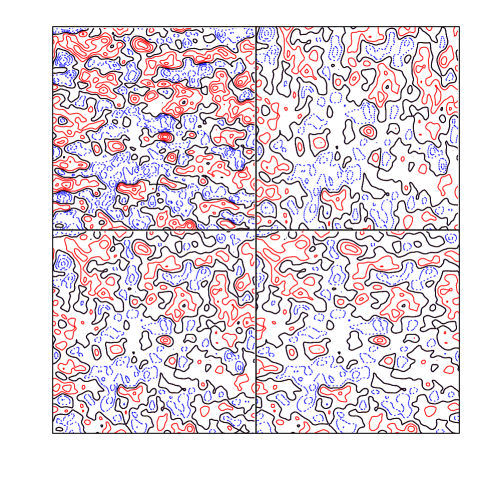
Figure 2: An illustration of the redshift and geometric distortions. The bottom left panel with the isotropic contours shows the density field in real space. The top left is the corresponding redshift space density field obtained from the linear relations (5) and (6) for a line of sight along the vertical axis. The top right and the bottom right panels illustrate geometric distortions parallel and perpendicular the line of sight, respectively. These geometric distortions are for a 25% difference between the assumed and true distances 25%.

In the remainder of this section we derive several relations for later use. The relation between redshift and real space correlations is invariant under an isotropic scaling transformation of the form ${\bf r}\rightarrow g{\bf r}$, where $g$ is a constant. Therefore, without loss of generality the effect of an incorrect choice of the cosmological parameters can be described by a transformation of the type ${\tilde{r}}_{\parallel}={r}_{\parallel}/(1+\alpha)$ and ${\tilde{\bf r}}_{\perp}={\bf r}_{\perp}$, where $(1+\alpha)$ is the ratio of the true value of $HD_{\rm A}$ to the assumed value. For clarity of notation, we place a tilde over functions defined in the space of ${\tilde{r}}_{\parallel}$ and ${\tilde{\bf r}}_{\perp}$. If $f=f({r}_{\parallel},{\bf r}_{\perp})$ then

$${\tilde{f}}({\tilde{r}}_{\parallel},{\tilde{\bf r}}_{\perp})\equiv f[({r}_{\parallel},{\bf r}_{\perp})]\;,$$ (13)

We can easily verify that the correlation function of $d$ computed in the space of $({\tilde{r}}_{\parallel},{\tilde{\bf r}}_{\perp})$ is

$${\tilde{\xi}}^{\mathrm{s}}({\tilde{r}}_{\parallel},{\tilde{\bf r}}_{\perp})=\xi^{\rm s}[(1+\alpha){\tilde{r}}_{\parallel},{\tilde{\bf r}}_{\perp}]\;.$$ (14)

According to (13), if $f=f(r)$ is independent of the direction of ${\bf r}$, then

$${\tilde{f}}\left({\tilde{r}}_{\parallel},{\tilde{\bf r}}_{\perp}\right)=f(r)$$ (15)

where $r=\sqrt{(1+\alpha)^{2}{\tilde{r}}_{\parallel}^{2}+{\tilde{\bf r}}_{\perp}^{2}}={\tilde{r}}\sqrt{(1+\alpha)^{2}{\tilde{\mu}}^{2}+(1-{\tilde{\mu}}^{2})}$. To first order in $\alpha$ we find

$${\tilde{f}}\left({\tilde{r}}_{\parallel},{\tilde{\bf r}}_{\perp}\right)=f({\tilde{r}})\left[1+\alpha{\tilde{\mu}}^{2}\frac{{\mathrm{d}}\ln f({\tilde{r}})}{{\mathrm{d}}\ln{\tilde{r}}}\right]\;.$$ (16)

We will also need the first order (in $\alpha$) relation

$$\mu^{2}={\tilde{\mu}}^{2}+2\alpha{\tilde{\mu}}^{2}(1-{\tilde{\mu}}^{2})\;.$$ (17)

between ${\tilde{\mu}}={\tilde{r}}_{\parallel}/{\tilde{r}}$ and $\mu={r}_{\parallel}/r$.

5 distortions in twenty one cm maps

We assume that $T_{\rm s}\gg T_{{}_{\rm CBR}}$ so that $\delta T_{\rm b}\propto x_{{}_{\rm HI}}(1+\delta^{\rm s})$ up to a multiplicative constant. We further substitute the expansion (2) for $x_{{}_{\rm HI}}$ and write $x_{{}_{\rm HI}}(1+\delta^{\rm s})\propto{\cal M}({{\bf r}})[1+(b-1)\delta^{\rm r}+\delta^{\rm s}]$ to first order in $\delta$, where $b=1+\partial\ln x_{{}_{\rm HI}}/\partial\delta$. Note that $x_{{}_{\rm HI}}$ is determined by the real space density $\delta^{\rm r}$, hence the appearance of $\delta^{\rm r}$. For simplicity we will assume that the data yields the quantity

$$d({\bf r})={\cal M}({\bf r})(1+\Delta^{\rm s})\;,$$ (18)

where $\Delta^{\rm s}=(b-1)\delta^{\rm r}+\delta^{\rm s}$. Using the linear relation (5) we find that $\Delta^{\rm s}=(b-1)\delta^{\rm r}+\delta^{\rm s}=b\delta^{\rm r}-{\mathrm{d}}U/{\mathrm{d}}r$ which can be identified as the redshift space density contrast corresponding to the real space density field $\Delta^{\rm r}=b\delta^{\rm r}$.

Figure 3: The correlation $\psi$ as a function of separation, for two values of the filling factor of ionized regions, as indicated in the figure. The upper ($F_{\rm f}=0.13$) and lower sets ($F_{\rm f}=0.36$) of curves are for sources identified as 4$\sigma$ and and $3.5\sigma$ peaks in the density field, respectively. The solid lines show the correlation when the mask of ionized regions is placed around the peaks, while the dotted lines are for masks displaced away from the peaks.

We write the data-data redshift space correlation function as

$$\psi^{\rm s}=<dd>={\cal C}_{{}_{\cal M}}(r)[1+\xi^{\rm s}({\bf r})]\;,$$ (19)

where ${\cal C}_{{}_{\cal M}}=<\cal MM>$ is the structure (correlation) function of the mask, and $\xi^{\rm s}$ is now the correlation function of $\Delta^{\rm s}$. We have also assumed that the mask $x_{{}_{\rm HI}}$ and $\delta$ are uncorrelated. This assumption is justified once the filling factor of ionized regions is larger than $\bar{n}R_{\rm c}^{3}$ where $\bar{n}$ is the number density of sources and $R_{\rm c}\sim\ {\rm h^{-1}Mpc}$ (comoving) is the coherence length of the correlations between the sources and the gas. This condition is easily satisfied as a single source is capable of ionizing relatively large regions around it. To test this assumption we have resorted to our random gaussian density field having a $\Lambda$CDM power spectrum (see figure 2). We identify the sources as peaks in the density smoothed with $1\ {\rm h^{-1}Mpc}$ and assume that each source ionizes a region of a given radius around it. These regions define our mask. A comparison between the correlation of the mask times the density field when the mask is placed around the sources and when it is placed randomly in the box serves as an indication to the the degree of correlation between the mask and the density field. In figure (3) the solid lines are the correlation function $\psi$ (in real space) for a mask placed around the sources while the dotted are the correlations when the mask is placed randomly in the box. The upper and lower sets of curves correspond to two values of the filling factor, $F_{\rm f}$, of ionized regions. The values $F_{\rm f}=0.13$ and $0.36$, respectively, correspond to sources identified as $4\sigma$ and $3.5\sigma$ peaks. The differences between the dotted and solid curves for each value of the $F_{\rm f}$ are negligible.

We will write now the expressions describing the anisotropy of the data-data correlation function in the presence of geometric and redshift distortions. We restrict the analysis to the linear regime $\delta\ll 1$ and to first order in $\alpha$.

We write $\tilde{\xi}^{\rm s}({\tilde{r}}_{\parallel},{\tilde{\bf r}}_{\perp})=\xi^{\rm s}((1+\alpha){\tilde{r}}_{\parallel},{\tilde{\bf r}}_{\perp})$ and use (7) to express $\xi^{\rm s}$ in terms of the moments $\xi_{l}(r)$ with ($r=\sqrt{(1+\alpha)^{2}{\tilde{r}}_{\parallel}^{2}+{\tilde{\bf r}}_{\perp}^{2}}$) and Legendre polynomials evaluated at $\mu=(1+\alpha){\tilde{r}}_{\parallel}/{\tilde{r}}$. Then we use (16) and (17) to expand $\xi_{l}$ and $P_{l}$ as functions of ${\tilde{r}}$ and ${\tilde{\mu}}$ to first order in $\alpha$. The final result of this straightforward algebra is

$${\tilde{\psi}}^{\rm s}\left({\tilde{r}}_{\parallel},{\tilde{\bf r}}_{\perp}\right)=\displaystyle\sum_{l=0,2,4}{{\psi}}_{l}({\tilde{r}})P_{l}({\tilde{\mu}})$$

$$+\alpha\displaystyle\sum_{l=0,2,4}{{\psi}}_{l}({\tilde{r}})\left[\frac{{\mathrm{d}}\ln{{\psi}}_{l}({\tilde{r}})}{{\mathrm{d}}\ln\tilde{r}}{\tilde{\mu}}^{2}P_{l}({\tilde{\mu}})+{\tilde{\mu}}(1-{\tilde{\mu}}^{2})\frac{{\mathrm{d}}P_{l}({\tilde{\mu}})}{{\mathrm{d}}{\tilde{\mu}}}\right]$$

$$=\displaystyle\displaystyle\sum_{l=0,2,4}\left[{{\psi}}_{l}({\tilde{r}})+\alpha a_{l}({\tilde{r}})\right]P_{l}({\tilde{\mu}})+\alpha a_{6}({\tilde{r}})P_{6}({\tilde{\mu}})\;\,$$ (20)

where $\psi_{{}_{0}}={\cal C}_{{}_{\cal M}}(1+\xi_{{}_{0}})$ and $\psi_{{}_{l}}={\cal C}_{{}_{\cal M}}\xi_{{}_{l}}$ for $l>0$, and

$$a_{0} = \frac{1}{3}\psi_{{}_{0}}\frac{{\mathrm{d}}\ln\psi_{{}_{0}}}{{\mathrm{d}}\ln{\tilde{r}}}+\psi_{{}_{2}}\left(\frac{2}{5}+\frac{2}{15}\frac{{\mathrm{d}}\ln\psi_{{}_{2}}}{{\mathrm{d}}\ln{\tilde{r}}}\right)$$

$$a_{2} = \frac{2}{3}\psi_{{}_{0}}\frac{{\mathrm{d}}\ln\psi_{{}_{0}}}{{\mathrm{d}}\ln{\tilde{r}}}+\psi_{{}_{2}}\left(\frac{2}{9}+\frac{11}{21}\frac{{\mathrm{d}}\ln\psi_{{}_{2}}}{{\mathrm{d}}\ln{\tilde{r}}}\right)$$

$$+ \psi_{{}_{4}}\left(\frac{20}{21}+\frac{4}{21}\frac{{\mathrm{d}}\ln\psi_{{}_{4}}}{{\mathrm{d}}\ln{\tilde{r}}}\right)$$

$$a_{4} = -\psi_{{}_{2}}\left(\frac{24}{35}-\frac{12}{35}\frac{{\mathrm{d}}\ln\psi_{{}_{2}}}{{\mathrm{d}}\ln{\tilde{r}}}\right)+\psi_{{}_{4}}\left(\frac{20}{77}+\frac{39}{77}\frac{{\mathrm{d}}\ln\psi_{{}_{4}}}{{\mathrm{d}}\ln{\tilde{r}}}\right)$$

$$a_{6} = -\psi_{{}_{4}}\left(\frac{40}{33}-\frac{10}{33}\frac{{\mathrm{d}}\ln\psi_{{}_{4}}}{{\mathrm{d}}\ln{\tilde{r}}}\right)\;.$$ (21)

The visual impression between geometric and redshift distortions seen in figure (2) is quantified by the relation (20). The moments $a_{l}$ and $\psi_{l}$, respectively, characterize the geometric and redshift distortions. A term containing $P_{6}$ is missing from the redshift distortions of the correlations. One could determine the correct value of the distance ratio, $\alpha$, by minimizing the square of the moment corresponding to $P_{6}$, independent of the details of the mask structure function ${\cal C}_{{}_{\cal M}}$. As we shall see below other moments can also be used to infer $\alpha$. Let us inspect the moments $a_{l}$ and $\psi_{l}$. The moments depend on the linear matter correlation function which we obtain from the power spectrum of the $\Lambda$CDM model with $\Omega_{\rm m}=0.3$. Figure (4) shows the ratio of the moments $a_{l}/\psi_{l}$ for $l=0,2$, and 4. Also shown is $a_{6}$ multiplied by a factor of 10 for the sake of clarity. To illustrate the differences arising from geometric and redshift distrotions, we assume that the mask structure function, ${\cal C}_{{}_{\cal M}}$, is unity. The ratio $|a_{0}/\psi^{0}|$ is small except at separations of $r\sim 60\ {\rm h^{-1}Mpc}$ where measuring the correlations is probably hard. The moments $a_{2}$ and $a_{4}$ are larger than $\psi_{2}$ and $\psi_{4}$ by a factor of $2$ and $10$, respectively, making the anisotropy pattern a very sensitive function of $\alpha$.

All moments $\int\psi^{\rm s}({\tilde{\mu}})P_{l}({\tilde{\mu}}){\mathrm{d}}{\tilde{\mu}}$ of the temperature correlation are expressed in terms of the functions ${\cal C}_{\cal M}$, $\xi_{{}_{0}}$, the redshift distortion parameter $\beta$ needed to express $\xi_{{}_{l}}$ in terms of $\xi_{{}_{0}}$, and the geometric distortion parameter, $\alpha$. A comparison between the moments should allow us to constrain $\alpha$, the bias parameter $\beta$, and the form of the mask. As explained previously the moment corresponding to $P_{6}$ arises only because of geometric distortions. Therefore, $\alpha$ can be constrained by minimizing the square of this moment independent of the mask and redshift space distortions. Further, one can assume parametric forms for ${\cal C}_{\cal M}$ and $\xi_{{}_{0}}$. The parameters of these forms as well as $\alpha$ and $\beta$ can then be obtained by fitting the moments as a function of $r$.

5.1 Validity of the approach

During the early stages of reionization the filling factor, $F_{\rm f}$, of ionized regions is small and the effect of the mask on the temperature correlations is negligible. Further, one can restrict the correlation analysis to large neutral patches extracted from 21 cm maps (figure 3 in Ciardi & Madau 2003). In the intermediate and late stages of reionization ($F_{\rm f}~{}\hbox to0.0pt{\raise 1.72218pt\hbox{$>$}\hss}{\lower 3.01385pt\hbox{$\sim$}}~{}0.5$), it will be increasingly difficult to extract large neutral regions from the data (Nusser et. al. 2002). During these stages, the temperature correlation from the full maps will probably need to be considered. The method outlined above is capable of treating these stages where the mask is to be considered. In developing the method we have made two important assumptions related to the mask. The first is that the mask-temperature correlation is negligible. The second is that peculiar motions do not introduce any systematic anisotropy in the shape of the mask boundaries, i.e., the ionization fronts. Once the typical size of ionized regions becomes larger than the correlation (coherence) length ($~{}\hbox to0.0pt{\raise 1.72218pt\hbox{$<$}\hss}{\lower 3.01385pt\hbox{$\sim$}}~{}1\ {\rm h^{-1}Mpc}$ at $z\sim 10$) of mass distribution the mask-temperature correlation is expected to be negligible. Figure 3 illustrates that the mask-signal correlation is indeed negligible once the ionized volume is large enough (corresponding to $F_{\rm f}~{}\hbox to0.0pt{\raise 1.72218pt\hbox{$>$}\hss}{\lower 3.01385pt\hbox{$\sim$}}~{}0.13$ in the example given in the figure). Let us now justify neglecting the effect of peculiar motions on the mask boundaries. The relative displacement of the boundary is $v/(aHR)$ where $R$ is the typical comoving size of the ionization front, and $v$ is the typical difference in physical peculiar velocity between two points at which a line of sight intersects the boundary. Also, $a=1/(1+z)$ and $H$ is the Hubble function at redshift $z$. For simplicity consider $\Omega=1$. In this case $v=v_{0}a^{2}H/H_{0}$ where $v_{0}$ and $H_{0}$ are $v$ and $H$ at $z=0$. The relative displacement is then $av_{0}/(H_{0}R)$. Taking $H_{0}R=1000$km/s which is appropriate for $F_{\rm f}~{}\hbox to0.0pt{\raise 1.72218pt\hbox{$>$}\hss}{\lower 3.01385pt\hbox{$\sim$}}~{}0.5$, $a=0.1$, and $v_{0}=100$km/s one gets a relative displacement of a few per cents. There is also an important factor which reduces any systematic distortions of the ionization fronts. For large ionized regions the the relative velocity $v$ can equally be positive as much as negative. This is because UV ionized bubbles are significantly larger than the coherence length ($\sim 1\ {\rm h^{-1}Mpc}$ at $z\sim 10$) of the dense regions near which the sources are likely to reside. Because of this symmetry in $v$, the mean distortions in the boundaries of bubbles tend to cancel out.

Figure 4: Ratios of the moments, $a_{l}/\psi_{l}$ ($l=0,2,4$), as a function of separation. Also shown is the moment $a_{6}$ multiplied by a factor of 10. All curves correspond to the linear correlation function of $\Lambda$CDM with $\Omega_{\rm m}=0.3$, assuming that the correlation of the mask is unity.

6 Alternative applications of the AP test

So far we have considered the anisotropies of the correlations in the diffuse neutral component. We now consider two alternative applications which are also promising and are practically unaffected by foreground contamination.

6.1 Dense peaks and minihalos

Consider a UV dominated reionization scenario. At any redshift, most of the 21 cm signal comes from the regions that have not yet been ionized. However, the already ionized regions are likely to contain high density peaks in which the neutral hydrogen is dense enough to produce significant 21 cm emission. For sufficient instrumental spatial resolution these peaks would show localized 21 cm emission engulfed in regions with practically no 21 cm signature at all. These peaks are particularly useful in the absence of 21 cm signal from diffuse neutral hydrogen towards the end of reionization. Provided that these peaks are at least marginally resolved, the statistical anisotropy of their shapes can be used to constrain the cosmological parameters. This application is along the lines of the classic AP test (Alcock & Paczyński 1979). Since the peaks are compact, foreground contamination is minimized in this way of applying the test. The velocity flow around the peaks is in the mildly non-linear regime and non-linear methods for modeling redshift distortions are needed.

The correlation function of the discrete distribution of the peaks could be computed. The anisotropy of this correlation could be used as a probe of geometric distortions (e.g. Ballinger, Peacock & Heavens 1996; da Ângela, Outram & Shanks 2005). Here again, foreground contaminations are irrelevant since the 21 cm maps are used merely for locating the peaks. One can also consider neutral gas in minihalos in which collisions could be efficient at raising the spin temperature above that of the CMB (Iliev et al 2002). They amount to significant 21 cm emission even before reionization. Here also once can apply the AP test to the distribution of these minihalos in 21 cm maps. The distribution of these peaks would also be affected by redshift distortions. The signature of these distortions here is also distinguishable from that of geometric distortions.

6.2 The patchy mask: ionization fronts

In a UV radiation dominated reionization, the mask made by ionized regions is patchy (see figure 3 of Ciardi & Madau 2002). The boundaries of these patches, i.e., the ionization fronts are marked by a sharp transition in 21 cm emission and should be possible to identify in future 21 cm maps. The shape of the ionization fronts could be used to probe geometric distortions. As we have seen in §5.1, the effect of peculiar motions on the anisotropy of the boundaries is negligible for large enough bubbles. Methods for identifying these boundaries in noisy maps observed with a given instrumental resolution must be developed. This is worthwhile since foreground contamination are not likely to affect the identification of these boundaries and also, by restricting the application to large ionized regions, redshift distortions can be made negligible.

7 Discussion

We have discussed the application of the Alcock-Paczyński test to maps of the redshifted 21-cm emission from the era of reionization. Our two main conclusions are a) at $z\sim 20$ the ratio of the frequency to angular distance scales is sensitive to the assumed cosmological parameters and the equation of state of the dark energy, and b) that geometric distortions resulting from an erroneous choice for the cosmological parameters are very distinct from redshift distortions caused by peculiar motions. Redshift distortions enhance the clustering along the line of sight while geometric distortions simply compress the density contours either along line of sight or the perpendicular direction. Judging by the ratio of the moments (see figure 4) a determination of the correlation of temperature fluctuations to an accuracy of $20\%$ should allow a successful application of the AP test. Prior to the end of reionization by UV sources large unionized regions should be easily distinguishable from the propagating ionized bubbles in 21 cm emission maps. Temperature correlation functions over scales up to several Mpcs can be computed reliably from these regions alone. Thus an application of the AP test to these correlations completely avoid dealing with the mask, $\cal M$. Nevertheless, for the sake of completeness we have presented results including the mask. The prospects for measuring the cosmological 21-cm signal are good in view of the planed telescopes like the Low Frequency Array (LOFAR), the Primeval Structure Telescope (Peterson, Pen & We 2005), and the Square Kilometer Array. It remains to be seen how well the correlation function will be determined from data provided by these telescopes.

A potential obstacle in extracting any cosmological signal from future 21 cm maps is contamination by bright extragalactic sources and Galactic synchrotron and free-free emision. (e.g. Oh & Mack 2003; Di Matteo et al. 2002; Di Matteo, Ciardi & Miniati 2004, Wang et al. 2005). Galactic contamination contributes about 70% (e.g. Wang et al. 2005). This component is believed to be a smooth function of frequency. If so then it would be possible to remove its contribution to the correlation function (or line of sight power spectrum) of the cosmological signal on small scales. The extragalactic point source contamination is more fluctuating than the Galactic component. But, as has been shown by Wang etal (2005), the total foreground contamination can be almost completely cleaned from the line of sight power spectrum of the 21 cm emission on scales with wavenumbers $\ll 0.1\rm h/Mpc$. Therefore, over a wide range of scales, foreground contaminations are not expected to pose a major problem for the application of the AP test and for extracting other cosmological information from 21 cm maps.

We have also outlined alternative method for application of the AP test. A promising method relies on identifying high density peaks in 21 cm. These peaks could be associated with minihalos which could lead to significant emission even before the onset of reionization. They could also result from neutral hydrogen in dense regions engulfed by the expanding ionized bubbles during the late stages reionization. Another method relies on the geometric distortions of the boundaries of patchy ionized regions, i.e. the reionization fronts. The advantage of these method is that they are not affected by foreground contamination since the 21 cm maps are used merely to locate the position of the peaks in the first method and the reionization fronts in the second.

A proper testing of the methodology developed here is beyond the scope of the current paper. Ideally one would like to use radiative transfer simulations of the reionization era. The problem, however, is that most of the simulation boxes are still too small for a proper statistical study of reionization. The largest simulation available to us is that of Ciardi & Madau 2003, having a cubic box of $20\ {\rm h^{-1}Mpc}$ on the side. We intend to use this simulation to study the distortions in the correlations and the shapes of the ionization fronts. An alternative to full radiative transfer simulations is the approximate methods developed by Benson et. al 2001 to model reionization using large N-body simulations. These methods will enable us to study the proposed application of the AP test to simulations of box size of $\sim 100\ {\rm h^{-1}Mpc}$.

8 Acknowledgment

The author wishes to than S. Zaroubi and A.G. de Bruyn for stimulating discussions. This work is supported by the Research and Training Network “The physics of the Intergalactic Medium” set up by the European Community under the contract HPRNCT-2000-00126 and by the German Israeli Foundation for the Development of Research. The author is grateful to the Institute for Advanced Study (Princeton) and the Institute of Astronomy (Cambridge) for the hospitality and support.

References

- [1] Alcock C., Paczyński B., 1979, Nature, 281, 358
- [2] da Ângela J., Outram P.J., Shanks, 2005, MNRAS, in press
- [3] Bahcall N.A., et al. , 2003, ApJ, 585, 182
- [4] Ballinger, W.F. Peacock J.A., Heavens A., 1996, MNRAS, 282, 877
- [5] Baltz E.A, Gnedin N.Y., Silk, J., 1998, ApJ, 493, 1
- [6] Barkana R., Loeb A., 2004, atsro-ph/0409572
- [7] Barreiro T., Bento M.C., Santos N.M., Sen A.A., 2003, Phys.Rev D, 68, 3515
- [8] Benson A.J., Nusser A., Sugiyama N., Lacey C., 2001, MNRAS, 320, 153
- [9] Bharadwaj S., Saiyed A.Sk., 2004, MNRAS, 352, 142
- [10] Bruscoli M., Ferrara A., Fabbri R., Ciardi B., 2000, MNRAS, 318, 1068
- [11] Caldwell R.R., Doran M., 2004, Phys.Rev D., 69, 3517
- [12] Caresia P., Matarrese S., Moscardini L., 2004, ApJ, 605, 21
- [13] Coble K., Dodelson S., Frieman J.A., Phys.Rev D, 55, 1851
- [14] Chen X., Miralda-Escude J., 2004, ApJ, 602, 1
- [15] Ciardi B., Madau P., 2003, ApJ, 596, 1
- [16] Cole A., Fisher K.B., Weinberg D.H., 1994, MNRAS, 267, 785
- [17] Croft R.A.C., Weinberg D.H., Bolt M., Burles S., Hernquist L., Katz N., Kirkman D., Tytler D., 2002, ApJ, 581, 20
- [18] Davis M., Peebles P.J.E., 1983, ApJ, 267, 465
- [19] Desjacques V., Nusser A., Haehnelt M.G., Stoehr F., 2004, MNRAS, 350, 879
- [20] Di Matteo T., Ciardi B., Miniati F., 2004, atro-ph/0402322
- [21] Di Matteo T., Perna R., Abel T., Rees M.J., 2002, ApJ, 564, 576
- [22] Field G.B., 1958, Proc, IRE, 46, 240
- [23] Field G.B., 1959, ApJ, 129, 551
- [24] Fisher K.B., Nusser A., 1996, MNRAS, 279, 1
- [25] Furlanetto S.R., Sokasian A., Hernquist L., 2004, MNRAS, 347, 187
- [26] Furlanetto S.R., Zaldarriaga M., Herquist L., 2004, ApJ, 613, 16
- [27] Gnedin N.Y., Shaver P.A., 2004, ApJ, 608, 611
- [28] Hamilton A.J.S., 1992, ApJ, 385, 5
- [29] Hatton S., Cole S., 1998, MNRAS, 296, 10
- [30] Hogan C.J., Rees M.J., 1979, MNRAS, 188, 791
- [31] Hui L., Stebbins A., Burles S., 1999, ApJ, 511, 5
- [32] Ikebe Y., Reiprich T.H., Böhringer H., Tanaka Y., Kitayama T., 2002 A&A, 383, 773
- [33] Iliev I.T., Shapiro P.R., Ferrar A., Hugo M., ApJ, 2002, 172, 123
- [34] Kaiser N., 1987, MNRAS, 227, 1
- [35] Knop R., et al. , 2003, ApJ, 598, 102
- [36] Knox L., Scoccimarro, R., Dodelson S., 1998, Phys.Rev D, 81, 2004
- [37] Kunz M., Corasaniti P.S., Parkinson D., Copeland E.J., 2004, Phys.Rev D, 70, 1301
- [38] Lima J.A.S., Alcaniz J.S., 2000, A&A, 357, 393
- [39] Madau P., Meiksen A., Rees M.J., 1997, ApJ, 475, 429
- [40] McDonald P., Miralda-Escudé J., Rauch M., Sargent W.L.W., Barlow T.A., Cen R., Ostriker J.P., 2000, ApJ, 543, 1
- [41] McDonald P., Seljak U., Cen R., Weinberg D.H., Burles S., Schneider D.P., Schlegel D.J., Bahcall N.A., Briggs J.W., Brinkmann J., Fukugita M., Ivezic Z., Kent S., Vanden Berk D.E., 2004, astro-ph/0407377
- [42] Nusser A., Haehnelt M., 2000, MNRAS, 313, 364
- [43] Nusser A., Davis M., 1994, ApJ, 421
- [44] Nusser A., Davis M., Willick J.A., 1996, ApJ, 473
- [45] Nusser A., Benson A.J., Sugiyama N., Lacey C., 2002, ApJ, 580, 93
- [46] Nusser A., 2005, MNRAS, 359, 183
- [47] Oh S.P., Mack K.J., 2003, MNRAS, 346, 871
- [48] Peebles P.J.E., The Large Scale Structure in the Universe, Princeton Univ. Press.Princeton, NJ
- [49] Peacock J.A., 1999, Cosmological Physics, Cambridge Univ. Press. Cambridge
- [50] Percival W.J., et al. , 2002, MNRAS, 337, 1068
- [51] Peterson J., Pen Ue-Li, Wu X.P., 2005, astro-ph/0502029
- [52] Ratra B., Peebles P.J.E., 1988, Phys.Rev D, 37, 3406
- [53] Ricotti M., Ostriker J., 2004, MNRAS,352, 547
- [54] Ricotti M., Ostriker J., Gnedin N.Y.,2004, astro-ph/0404318
- [55] Riess A., et al. , 2004, ApJ, 607, 665
- [56] Scott D., Rees M.J., 1990, MNRAS, 247, 510
- [57] Spergel D.N. et al. , 2003, ApJS, 148, 175
- [58] Strauss M.A., Willick J.A., 1995, Phys.Rep., 261, 271
- [59] Sunyaev R.A., Zel’dovich Y.A., 1975, MNRAS, 171,375
- [60] Subramanian K., Padmanabhan T., 1993, MNRAS, 265, 101
- [61] Taylor A.N., Hamilton A.J.S., 1996, MNRAS, 282, 767
- [62] Tegmark M., et al. 2004, ApJ, 606, 702
- [63] Turner M.S., White M.J., Phys.Rev. D, Lett. 80, 1582
- [64] Tozzi P., Madau P., Meiksin A., Rees M.J., 2000, ApJ, 528, 597
- [65] Vauclair S.C., Blanchard A., Sadat R., Bartlett J.G., Bernard J.P., Boer M., Giard M., Lumb D.H., Marty P., Nevalainen J., 2003, A&A, 412, 37
- [66] Viel M., Weller J., Haehnelt M., 2004, astro-ph/0407294
- [67] Wetterich C., 1995, A&A, 301, 321
- [68] Wang X., Tegmark M., Santos M., Knox Lloyd, 2005, astro-ph/0501081
- [69] Wild J.P., 1952, ApJ, 115, 206
- [70] Zaldarriaga M., Furnaletto S.R., Hernquist L., 2004, ApJ, 608, 622
- [71] Zaroubi S., Hoffman Y., 1996, ApJ, 462, 25
- [72] Zaroubi S., Bernardi M., da Costa L.N., Hoffman Y., Alonso M.V., Wegner G., Willmer C.N.A., Pellegrini P.S., 2001, MNRAS, 326, 375
- [73] Zaroubi S., Silk J., 2005, MNRAS, 360, 64
- [74] Zehavi E., et al. , 2002, ApJ, 571, 172