Physics of Outflows: the Binary Protostar L 1551 IRS 5 and its Jets

Abstract

Recent observations of the deeply embedded L 1551 IRS 5 system permit the detailed examination of the properties of both the stellar binary and the binary jet. For the individual components of the stellar binary, we determine their masses, mass accretion rates, effective temperatures and luminosities. For the atomic wind/jet flow, we determine the mass loss rate, yielding observationally determined values of the ratio of the mass loss to the mass accretion rate, $f$. For the X-ray emitting region in the northern jet, we have obtained the jet-velocity and derive the extinction and the densities on different spatial scales. Examining the observational evidence within the framework of the x-wind theory leads us to conclude that these models are indeed potentially able to account for the observational data for this deeply embedded source.

1 Introduction

Since their discovery nearly three decades ago, the unexpected phenomenon of outflows in star forming regions has remained essentially unexplained. In particular, the processes responsible for the acceleration and collimation of the flows present one of the major unsolved problems of modern astrophysics (Lada, 1985; Shu et al., 1987, 2000; Eislöffel et al., 2000; Königl & Pudritz, 2000). Considerable progress has been made in the theoretical field, but observational results had generally been of too poor quality to make direct comparisons meaningful. In this paper, we examine recent various observational results for the deeply embedded source L 1551 IRS 5, which, when put together, finally permit the detailed comparison with theoretical models. Optically visible young stellar objects (lower mass loss and accretion rates) have previously been addressed by, e.g., Shang et al. (2002, and references therein).

Over the years, IRS 5 has enjoyed a variable status of ‘the archetypical CO outflow source’ and that of ‘a pathological case’ (e.g.,  Padman et al., 1997). More recently, renewed interest in this object has arisen, in part due to the recognition of its duplicity, as binarity seems to be a very frequent phenomenon among powerful outflow drivers (M. Barsony, private communication). If protostellar binarity is indeed intimately related to the physics of generating bipolar outflows, then one obviously wishes to understand the physics of the binary itself. We devoted therefore quite some effort to arrive at the understanding of the IRS 5 system. Based on the theory of protostellar structure and evolution, we find a solution capable of explaining observed characteristics of both IRS 5 itself and its associated jet flows, and which, when applied to x-wind models, successfully recovers the physical properties of the jets. Thus, in this particular case, a direct dependence on source binarity is not evidenced, as the theory of x-winds has been developed for single stellar objects.

The organisation of this paper is as follows: In Sect. 2, we review the evidence based on recent observations in both the optical, infrared and radio spectral regimes. In Sect. 3, we use published models of protostellar structure and evolution to derive the physical properties of the individual binary components and apply x-wind theory to derive some parameters relevant in the present context. In Sect. 4, we discuss our results and, finally, in Sect. 5, we briefly summarise our main conclusions.

2 The Observational Evidence

2.1 Mass loss rates from the large scale atomic flow

Hollenbach (1985) proposed that the luminosity of the [O i] 63 $\mu$m line can be used to estimate the wind mass loss rate. At the distance of 150 pc and for the observed line luminosity with an 86^′′ beam (White et al., 2000), this method would yield a mass loss rate of $8\times 10^{-7}$ $M_{\odot}\,{\rm yr}^{-1}$. In contrast, based on H I 21 cm observations of the redshifted gas with the VLA (Very Large Array, $\sim$ 57^′′ beam), Giovanardi et al. (2000) determined the mass loss rate from IRS 5 for the atomic wind as Ṁ${}_{\rm w,\,red}=1\times 10^{-6}$ $M_{\odot}\,{\rm yr}^{-1}$. Given the momentum symmetry of the red- and blueshifted flows (see their Table 2), a mass loss rate of about $2\times 10^{-6}$ $M_{\odot}\,{\rm yr}^{-1}$ seems indicated, a factor of three higher than that based on the [O i] 63 $\mu$m line.

The reason for this discrepancy is not entirely clear. One possibility could be that the condition, in which the Hollenbach relation is thought to hold, is not met by the flow from IRS 5 (viz. $\Phi_{\rm H}$ $\stackrel{{\scriptstyle<}}{{{}_{\sim}}}$ $n_{\rm 0,\,5}\,v_{\rm s,\,100}$, where $\Phi_{\rm H}$ is the particle flux in cm^-2 s^-1 through the shock front, and when the pre-shock density $n_{\rm 0}$ is expressed in units of $10^{5}$ cm^-3 and the shock velocity $v_{\rm s}$ is in units of 100 km s^-1). To some degree this might be supported by the fact that IRS 5 falls out completely, by more than one order of magnitude, of the empirical $L_{\rm forbidden\,line}-L_{\rm bol}$ relation found for a large number of jet-sources (Edwards et al., 1993; Liseau et al., 1997). However, most of these sources, being of T Tauri type, are presumably at a later stage of development.

Source variability could be another, perhaps more likely, reason and in which case neither of the two Ṁ_w estimates would be entirely correct, since both methods are based on the assumption of stationarity. Intensity variations from the shocked gas on small spatial and temporal scales ($\stackrel{{\scriptstyle<}}{{{}_{\sim}}}$ 10^′′, $<0.5$ yr) have frequently been observed (Cameron & Liseau, 1990; Liseau et al., 1996) and the [O i] 63 $\mu$m cooling time is likely of this order. As discussed by Giovanardi et al. (2000), the H I data pertain to time scales of the order of 30 yr and the memory of small scale variations might become ‘ironed out’ in the global flow.

2.2 The small scale flows

2.2.1 The velocities of the optical jets

On the sub-arcsec to ten arcsec scale, two independent jets from IRS 5 have been identified in the optical and in the near infrared (Fridlund & Liseau, 1998; Itoh et al., 2000; Fridlund et al., 2004). These have been designated as the ‘northern’ and the ‘southern’ jet, respectively. The two jets distinguish themselves by very different emissivity and velocity characteristics. The intensity of the northen jet is much stronger and the material exhibits much larger velocities. At the projected jet position 2^′′ (300 AU) distant from IRS 5, Fridlund et al. (2004) have recently obtained a maximum (blue-shifted) radial velocity of $\max v_{\rm rad}=v\cos{\theta}=430$ km s^-1. This flow velocity has been maintained at this high level over the years (cf. Stocke et al., 1988). Radial velocity and proper motion data imply that the jet is moving at non-zero angles with respect to the line of sight, i.e. $\theta_{\rm N}>0$ (Liseau & Sandell, 1986; Stocke et al., 1988; Fridlund & Liseau, 1994; Lucas & Roche, 1996), so that the jet velocity is strictly higher than 430 km s^-1, consistent with the shock generated X-ray luminosity observed from this jet position (Favata et al., 2002; Bally et al., 2003; Fridlund et al., 2004). In contrast, the radial velocity observed for the southern jet is at most 65 km s^-1 (Fridlund & Liseau, 1998; Hartigan et al., 2000; Pyo et al., 2002; Fridlund et al., 2004) and any non-zero proper motion is below detectability in the multi-epoch data of Fridlund et al. (2004).

2.2.2 The densities of the northern optical jet

At the position of observed highest radial velocity, Fridlund et al. (2004) have estimated local volume densities from spectrophotometric observations of lines of [S II], viz. $n_{\rm e}=(1.8\pm 0.4)\times 10^{3}$ cm^-3. This value represents the averaging over a region of effective radius 170 AU.

For this region of the northern jet, Itoh et al. (2000) have obtained a spectrum in the wavelength interval 1.05 to 1.82 $\mu$m and identified eight [Fe II] lines. These lines would be less affected by intervening extinction than the optical [S II] lines. Also, as noted by Itoh et al. (2000), most critical densities (ratio of radiative to collisional rates) for [Fe II] are higher than those of [S II]. Consequently, the [Fe II] lines trace potentially gas at higher densities.

We have extended the analysis by Itoh et al. (2000) by model fitting their entire observed spectrum, using an [Fe II] model atom having 142 energy levels with 1438 transitions and with atomic data from Quinet et al. (1996) and Zhang & Pradhan (1995). The absolute flux calibration was kindly communicated to us by Y. Itoh. The transitions under consideration are identified in the energy level diagramme of Fig. 1.

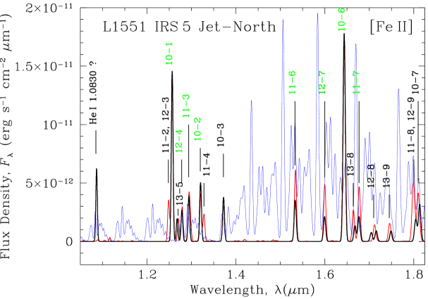
Figure 2: The observed and synthetic spectra of the northern jet in the photometric J- and H-bands. The black curve corresponds to the flux densities calculated from the line flux observations of Itoh et al. (2000, Table 1, ID=Eb, $R_{\lambda}=280$), who identified 8 [Fe II] lines, the transitions of which are labelled in green (cf. Fig. 1). Other line fluxes were estimated from their Fig. 5. The fitted model is shown in red: whereas the matching in the J-band is excellent, some of the weaker lines in the H-band appear too strong in the model. This ‘mis-fit’ could be due to insufficient background correction. The OH lines are particularly intense in this wavelength region, as is illustrated by the blue spectrum, showing the arbitrarily scaled telluric OH emission (Rousselot et al., 2000). Since X-ray emission has been detected from this jet position (Favata et al., 2002; Bally et al., 2003; Fridlund et al., 2004), we tentatively identify the emission feature at 1.08 $\mu$m as the recombination line ${\rm He\,I}\,\lambda 1.0830$ (${}^{3}{\rm P}^{0}\,2{\rm p}\,-\,^{3}{\rm S}\,2{\rm s}$).

Our best fit model is shown in Fig. 2 for the spectral resolution of 280 (Itoh et al., 2000). These calculations assume a Full Width Half Maximum of 150 km s^-1 for the [Fe II] lines (Pyo et al., 2002; Fridlund et al., 2004), solar chemical composition and an electron temperature $T_{\rm e}=10^{4}$ K. Little is known about the abundances in the jet, but the assumption of a solar iron abundance seems not too unreasonable (Beck-Winschatz & Böhm, 1994; Böhm & Matt, 2001). The absence of lines from highly excited states in the observed spectrum limits the temperatures to significantly below $3\times 10^{4}$ K, a regime in which the final results are not critically sensitive to the assumed temperature.

For optically thin emission (verified by the model calculations), the line ratio $I_{1.64\,\mu{\rm m}}/I_{1.25\,\mu{\rm m}}={\rm constant}=0.96$. For an average interstellar extinction law (Rieke & Lebofsky, 1985), the observed line ratio of 1.6 implies a visual extinction, $A_{\rm V}$, of 5.72 magnitudes. This value is consistent with the absence of detectable Paschen line emission, based on the H$\alpha$-flux of Fridlund et al. (2004), $F_{\alpha}=4\times 10^{-15}$ erg cm^-2 s^-1, and on Case B recombination (Hummer & Storey, 1987). This $A_{\rm V}$-value is also an upper limit, since for higher values, the P$\beta\,\lambda\,1.2818$ $\mu$m line would be readily seen in the spectrum of Itoh et al. (2000). Similar applies to P$\gamma\,\lambda\,1.0938$ $\mu$m.

With the extinction fixed, the fitting of the observed spectrum results in a local jet density, formally, as $\log n_{\rm e}=4.88\pm 0.02$, i.e. $(7.6^{+0.3}_{-0.4})\times 10^{4}$ cm^-3, for $1\sigma$ observational errors (Itoh et al., 2000). These densities in the northern jet are much higher than what can be determined for the southern jet.

The source size of this model is 60 AU (jet diameter = 0$\stackrel{{\scriptstyle\prime\prime}}{{{}_{\bf\cdot}}}$4), the column density is $N_{\rm[Fe\,II]}=2\times 10^{15}$ cm^-2 and the total [Fe II] cooling rate is $L_{\rm[Fe\,II]}=7\times 10^{-4}$ $L_{\odot}$ ($2.7\times 10^{30}$ erg s^-1).

2.2.3 The radio jets

On the 0$\stackrel{{\scriptstyle\prime\prime}}{{{}_{\bf\cdot}}}$1 to arcsec scales, Rodríguez et al. (2003a) have recently confirmed the binarity of the L 1551 IRS 5 jet also at radio wavelengths (3.5 cm). The radio jets appear well aligned with their optical counterparts which become detectable only further ‘down-stream’, because of heavy extinction. Given that the northern jet is the dominant one at most wavelengths, it might seem enigmatic that the 3.5 cm emission from the southern jet is stronger by a factor of about two. For free-free emission, a relatively mild, by a factor of $\sqrt{2}$, variation of the electron density, integrated along the line of sight ($S_{\nu,\,{\rm free-free}}\propto\int(x_{\rm e}n_{\rm H})^{2}\,{\rm d}l$), could accomplish this. The southern jet does not conform with the generally adopted idea about the disk-jet geometry, as its direction appears to deviate substantially from the expected orthogonality (Rodríguez et al., 2003a).

2.3 Properties of the binary protostar

On the basis of high resolution VLA observations at millimeter wavelengths, Rodríguez et al. (1998) resolved the central source IRS 5 into two components. The marginally resolved emission peaks have an elliptical appearance and most likely represent circumstellar disks around each of the components in a protostellar binary system. The protostars themselves are, of course, not directly detected at the wavelength of 7 mm.

2.3.1 The photospheric spectrum

The spectroscopic observations of the nebulosity HH 102 (S 239) by Mundt et al. (1985) revealed the reflected photospheric spectrum of the deeply embedded object IRS 5. The wavelength range was extended by Stocke et al. (1988), who concluded that the data were consistent with stellar spectral types of giants (luminosity class III) ranging from G2 (in the blue spectral range) to K0 (in the green spectral region), with an uncertainty of two sub-classes. In addition, the absorption line depths were indicative of a surface gravity even lower than that of supergiant stars (luminosity class I). Taken to the extremes, this would allow for a considerable range in photospheric temperatures, viz. from 4300 K (K2 I) up to 5600 K (G0 III), see, e.g., Cox (1999). In our analysis below, we will adopt a slightly less conservative range, viz. $T_{\rm eff}=(5100\pm 200)$ K, which covers the spectral types K0 III to G0 III and which includes the temperatures of supergiants of earlier spectral type. Stocke et al. (1988) interpreted this drift in spectral type, in combination with the low gravity, as evidence for an FU Orionis (FUOR) type of disk around IRS 5.

As already noted by Mundt et al. (1985), and reinforced by Stocke et al. (1988), the Balmer line profiles exhibit P Cygni structure, indicative of a wind velocity of about 440 km s^-1, essentially identical to the H$\alpha$ line width observed by Fridlund et al. (2004) in emission from the northern jet.

2.3.2 The radiative luminosity

For a distance of 150 pc, detailed and self-consistent fitting of the entire observed spectral energy distribution (SED) of IRS 5, using a two-dimensional radiative transfer model for a disk structure, led to the determination of the total luminosity, $L_{\rm tot}=40$ $L_{\odot}$ (White et al., 2000). This value is larger by nearly 40% than the calorimetric luminosity, $L_{\rm cal}=30$ $L_{\odot}$, obtained from direct integration of the SED, owing to photon escape in the low-density polar directions. The model also correctly reproduces observed spatial intensity profiles and interferometric visibilities, lending further confidence in the luminosity estimate by White et al. (2000).

2.3.3 The dynamical mass of the system

From multi-epoch radio observations of the proper motions of the binary source IRS 5, Rodríguez et al. (2003a) have estimated the dynamical mass of the system as $0.1\leq\sum_{i}m_{\star,\,i}+\sum_{i}m_{{\rm D},\,i}\sim 1.2$ $M_{\odot}$. The mass of the disks $\sum_{i}m_{{\rm D},\,i}=0.1$ $M_{\odot}$, with the northern disk being twice as massive as the southern one (Rodríguez et al., 1998).

3 Protostar models

For observationally derived values of $\theta$ (45^∘ to 60^∘, Sect. 2.2.1), the velocity of the northern jet, $>600$ km s^-1, is comparable to the escape velocities of main-sequence stars, given by

$$v_{\rm esc}=617.7\left(\frac{M}{R}\right)^{1/2}\hskip 5.69046ptM_{\odot}^{-1/2}\,R_{\odot}^{1/2}\,{\rm km\,s}^{-1}$$ (1)

with obvious notations. Since the combined mass of the binary amounts to about 1 $M_{\odot}$, the total luminosity should not exceed 1 $L_{\odot}$, if the stellar components were in the main-sequence. This is inconsistent with observation ($L_{\rm tot}=40$ $L_{\odot}$) and attests to the pre-main-sequence nature of the objects. One notes that this luminosity, on the one hand, is much too low for a typical FUOR, but also much too high for a T Tauri star, on the other.

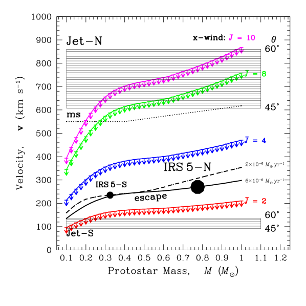
Figure 7: Various velocities versus protostellar mass. The deprojected radial velocities of the jets from L 1551 IRS 5 are shown by the shaded regions labelled Jet-N and Jet-S, respectively. The dots denote the positions of the corresponding driving sources, viz. the primary IRS 5-N and its less massive companion IRS 5-S. These are shown on curves of the escape velocity, corresponding to their mass accretion rates of $6\times 10^{-6}$ and $2\times 10^{-6}$ $M_{\odot}\,{\rm yr}^{-1}$, respectively. For comparison, the escape velocities for the main-sequence (ms) are also shown by the dotted line. The curves with the upper limit symbols are the loci of the asymptotic x-wind velocity for different values of the angular momentum parameter $\overline{J}$ and the accretion rate of $6\times 10^{-6}$ $M_{\odot}\,{\rm yr}^{-1}$. To reach velocities as high as those of Jet-N, large values of $\overline{J}$ are required, implying $f$-values of 0.3 or smaller (see the text).

It is illustrative to try to place IRS 5 into the H-R diagram, as shown in Fig. 7 of Stahler et al. (1980), where it would be somewhere near the top of the curve labelled ‘gas photosphere’. This would also be consistent with the age of the large scale molecular outflow, viz. $\sim 10^{5}$ yr (Snell et al., 1980; Padman et al., 1997). In the figure by Stahler et al. (1980), the evolutionary tracks for the protostellar ‘dust’ and ‘gas photosphere’, respectively, are separated. However, unlike their case of isotropic emission, the protostellar photosphere of IRS 5 can be viewed in reflection, since the dust ‘shell’ is not optically thick in all directions.

At the time Stocke et al. (1988) wrote their article, the binary nature of IRS 5 was not established. As an alternative to their suggestion, we shall below explore the possibility that the scattered light observed by Mundt et al. (1985) and Stocke et al. (1988) is due to the combined spectrum of two protostellar photospheres.

3.1 The mass-radius relations and accretion luminosities

At present, only the total luminosity, $L_{\rm tot}$, of the IRS 5 system is determined observationally. Assuming that the binary is protostellar in nature and, as such, derives its luminosity mostly from mass accretion processes, the total luminosity is the sum of the accretion luminosities of each of the members of the system, i.e., with common notations,

$$L_{\rm tot}=\sum_{i}L_{{\rm acc},\,i}=G\sum_{i}\dot{M}_{{\rm acc},\,i}\left(\frac{M}{R}\right)_{i}\hskip 5.69046pt.$$ (2)

We assume that the stellar contribution to $L_{\rm tot}=40$ $L_{\odot}$ (White et al., 2000) is provided by two objects of total mass, $M_{\rm tot}=1.1$ $M_{\odot}$ (Rodríguez et al., 2003b), with a minimum mass of about 0.1 $M_{\odot}$ for one of the components. Thus, for the examination of Eq. 2, we can limit the mass range for the individual masses to $M_{i}\in\left[0.1,\,1.0\right]$ $M_{\odot}$. This is ‘fortunate’, since in this mass interval the mass-radius relation, yielding the ratio $(M/R)_{i}$ for a given mass accretion rate $\dot{M}_{{\rm acc},\,i}$, is insensitive to the details of the accretion processes and physical boundary conditions (see Stahler, 1988; Palla & Stahler, 1992, 1993, and Fig. 3), provided these objects are in their deuterium burning stage.

The cited references provide mass-radius relations, $R(M)$, for a few mass accretion rates. For other values, we obtained the mass-radius relations by interpolating in between these rates (see Fig. 3).

3.2 The surface luminosities and effective temperatures

The effective temperatures of the protostellar photospheres are obtained from (Stahler, 1988; Palla & Stahler, 1993)

$$T_{{\rm eff},\,i}=\left(\frac{L_{{\rm surf},\,i}}{4\pi\sigma R_{i}^{2}}\right)^{\frac{1}{4}}\hskip 5.69046pt,$$ (3)

where the surface luminosity, $L_{{\rm surf},\,i}$, is the sum of the radiative and convective contributions, given by

$$L_{{\rm surf},\,i}=L_{{\rm rad},\,i}+L_{{\rm conv},\,i}\sim L_{0}\,\sqrt{\frac{(M/M_{\odot})_{i}^{11}}{(R/R_{\odot})_{i}}}+L_{{\rm D},\,i}\hskip 5.69046pt,$$ (4)

with $L_{0}=0.153$ $L_{\odot}$, and where we have approximated $L_{{\rm conv},\,i}$ with the luminosity during full deuterium burning, $L_{{\rm D},\,i}$. For accretion rates different from those given by Stahler (1988), $L_{{\rm D},\,i}$-values were obtained by interpolating the published $L_{\rm D}(M)$-curves. Since our primary objective is to obtain some reasonable estimates of $T_{{\rm eff},\,i}$, we did not bother to attempt extrapolating the $L_{\rm D}(M)$-curves beyond those given by Stahler (1988). Instead, for $1.1\times 10^{-5}$ to $1.5\times 10^{-5}$ $M_{\odot}\,{\rm yr}^{-1}$ we used the curve for $1\times 10^{-5}$ $M_{\odot}\,{\rm yr}^{-1}$, a procedure which will not affect our conclusions below.

3.3 Physical parameters of the binary components

We examine numerically Eq. 2 on the intervals $M_{i}\in\,[0.1,\,1.0]$ $M_{\odot}$ and $\dot{M}_{{\rm acc},\,i}\in[2,\,15]\,10^{-6}$ $M_{\odot}\,{\rm yr}^{-1}$, within which the parameters for both binary components are allowed to vary on the adopted grid, $\delta M=0.025$ $M_{\odot}$ and $\delta\dot{M}_{\rm acc}=1.0\times 10^{-6}$ $M_{\odot}\,{\rm yr}^{-1}$, respectively. This discretisation introduces a ‘fuzziness’ on the boundary condition $L_{\rm tot}=40$ $L_{\odot}$, which we estimate from $(\Delta L/L)_{\rm acc}\sim\pm[(\partial M/M)^{2}+(\partial\dot{M}/\dot{M})^{2}+(\partial R/R)^{2}]^{1/2}$ as about $\pm 15\%$ ($\pm 5.8$ $L_{\odot}$). This is comparable to the observational uncertainty. As an additional constraint, the effective temperature of the more luminous component is bounded by the interval $T_{{\rm eff},\,i}\in\,[4900,\,5300]$ K (see Sect. 2.3.1).

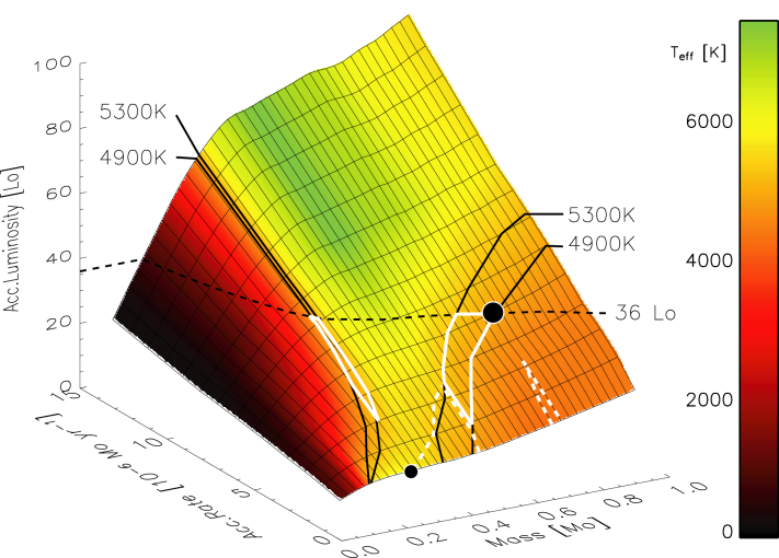
Figure 4: The explored parameter space in the variables mass accretion rate, accretion luminosity, effective temperature and protostellar mass. Here, the radii of the protostar models are implicit and presented separately in Fig. 3. The bar to the right of the graph provides the colour coding for the effective temperature. Areas, thought best to represent the protobinary L 1551 IRS 5 are encompassed by the white lines, where the full-drawn lines indicate the positions of the primaries and the dashed lines those of the companions. The smaller and clearly separated areas correspond to pairs in which the less massive star is the more luminous object. The black lines are meant to facilitate the viewer’s orientation along the axes. Our best solution for the IRS 5 binary is shown by the fat black dots, with the bigger one identifying the primary (IRS 5-N, see the text).

We find a couple of islands of formally acceptable solutions, shown in Fig. 4. There, the explored parameter space for the variables mass, accretion rate, accretion luminosity and effective temperature is depicted. Most solutions select the more massive star (the ‘primary’) as also the more luminous one. This is shown by the larger area encompassed by the full-drawn white curve. The adjacent dashed lines outline the region, where the corresponding secondaries are situated.

A smaller number of other solutions were also found, where the less massive star (the ‘secondary’) is the more luminous one, because of a much larger mass accretion rate (and, hence, becomes the primary in the commonly accepted sense). These are shown by the two separated islands.

Our preferred solution is shown in Fig. 4 by the two black dots, where the larger one signifies the primary (both more massive and more luminous). The reasons for this selection will become apparent below. The physical parameters for the protostellar primary of IRS 5 are: $M_{1}=0.8$ $M_{\odot}$, $\dot{M}_{{\rm acc,}\,1}=6\times 10^{-6}$ $M_{\odot}\,{\rm yr}^{-1}$, $T_{\rm eff,\,1}=4.9\times 10^{3}$ K, $\log g_{1}=3.1$ and $v_{\rm esc,\,1}=270$ km s^-1. For the secondary, the corresponding values are $M_{2}=0.3$ $M_{\odot}$, $\dot{M}_{{\rm acc,}\,2}=2\times 10^{-6}$ $M_{\odot}\,{\rm yr}^{-1}$, $T_{\rm eff,\,2}=5.8\times 10^{3}$ K, $\log g_{2}=3.2$ and $v_{\rm esc,\,2}=235$ km s^-1, respectively. The secondary contributes 25% to the total luminosity and the derived values of $\log g$ correspond to those of normal giants (luminosity class III, cf. Sect. 2.3.1).

3.3.1 Photospheric emission

The parameters derived in the previous section can be used to predict the photospheric spectra of IRS 5. Simple estimates of the resulting monochromatic luminosities indicate that the photospheric emission of the hotter secondary should be comparable in intensity to that of the cooler primary in the blue spectral region, but weaker already in the green (and for longer wavelengths). This is verified in detail when examining theoretical stellar atmosphere models. We use the NextGen models of Hauschildt et al. (1999) for the appropriate effective temperatures, the closest available values of the surface gravity ($\log g=3.5$) and solar chemical composition.

The individual model spectra and their sum are shown in Fig. 5, whereas in Fig. 6, the normalized composite model spectrum is displayed together with the observations by Stocke et al. (1988). The latter models have been ‘spun up’ to the escape velocities of the individual components prior to adding them together. These velocities must be regarded as upper limits to real and observable rotation speeds (break-up and viewing geometry, respectively), but these values are consistent with the limited spectral resolution of the observations of Stocke et al. (1988).

Rotation at, or rather close to, break-up in the stellar equatorial regions would also naturally explain the extreme supergiant characteristics of some of the absorption lines, since in this case, $\log g$ corresponds by definition to zero gravity.

For the interpretation of the nature of IRS 5, the implications of the FUOR-disk and protostellar photosphere scenarios are very different. High resolution spectroscopy in the optical should enable us to distinguish between these alternate models and, furthermore, potentially provide the opportunity to study stellar surfaces during an evolutionary phase which has not previously been accessible to direct observation.

3.4 Outflow models

To put the observed and derived properties of the binary protostar and the binary jet into context, we will make use of theoretical models of outflows. Specifically, the theory of magnetocentrifugally driven flows (x-winds) has been worked out in considerable detail and presented by F. Shu and co-workers in a series of papers.

3.4.1 x-wind velocities

In terms of the mass-radius relation (Sect. 3.1), the expression for the terminal wind velocity by Shu et al. (1994, their Eq. 4.13a) can be recast into

$${\overline{v}}_{\rm w}\leq\left[\,\frac{2\,{\overline{J}}-3}{r_{x}}\,\,G\,\left(\frac{M}{R}\right)\right]^{1/2}\hskip 5.69046pt,$$ (5)

where $r_{x}$ is a factor, such that $r_{x}$ times the stellar radius $R$ is the radial distance of the location of the x-point, assumed to be close to the radius of corotation of the stellar surface and the circumstellar Keplerian disk, so that $r_{x}$ is of order unity. The star is assumed to rotate near break-up.

As explicitly indicated, Eq. 5 represents an upper limit to the wind velocity, with equality reached at infinity (Shu et al., 1995). The angular momentum parameter, ${\overline{J}}$, takes values $>1.5$ and is likely not to exceed $\sim 10$. For the mass-radius relation corresponding to the accretion rate of $6\times 10^{-6}$ $M_{\odot}\,{\rm yr}^{-1}$ (Fig. 3), graphs of Eq. 5, with $r_{x}=1.0$, are shown in Fig. 7.

3.4.2 x-wind $f$-factors and densities

For a single stellar mass and a particular choice of parameters ($M=0.5$ $M_{\odot}$, $R=4$ $R_{\odot}$, $r_{x}=1.0$, Ṁ${}_{\rm w}=10^{-6}$ $M_{\odot}\,{\rm yr}^{-1}$), Najita & Shu (1994) presented detailed numerical results, covering the range in $\overline{J}$ from 2.0 to 7.8, with accompanying magnetic field strengths from 1.5 to 8.3 kG. Corresponding $f$-factors vary from 0.4 to 0.1, where $f$ is defined as the ratio of the mass loss to the mass accretion rate.

The collimation of, initially wide-angled, x-winds into narrow jets has been addressed by Shu et al. (1995). These authors also make a theoretical prediction of the density profile across the jet, i.e. in terms of the jet radius, the density scales approximately as $\rho(r)\propto r^{-2}$.

4 Discussion

4.1 The deuterium abundance

The results presented for the protostar binary IRS 5 are based on the mass-radius relations during deuterium burning as provided by the models of Stahler (1988) and Palla & Stahler (1992). These were calculated for the deuterium abundance relative to hydrogen, ${\rm[D/H]}=2.5\times 10^{-5}$, and are, as such, sensitive to the assumed [D/H].

Recent observations indicated the significantly lower value of about $1.5\times 10^{-5}$ in the solar neighbourhood and, furthermore, with a considerable dispersion (Sonneborn et al., 2002; Moos et al., 2002; Steigman, 2003). However, Linsky & Wood (2004) recently announced that they could reconcile the observational data with a value of ${\rm[D/H]}=(2.3\pm 0.4)\times 10^{-5}$ within 1 kpc of the Sun, in which case the results of the calculations by Stahler (1988) and Palla & Stahler (1992), with regard to the assumed deuterium abundance, remain valid.

4.2 Single-star theory and binary system

We obtain a binary mass ratio of $q=M_{2}/M_{1}\sim 0.4$, which is close to the peak of the observed distribution for solar-type stars in the solar neighbourhood (Duquennoy & Mayor, 1991). These authors did also not find any statistically significant dependence of the $q$-distribution on binary period (hence, binary separation).

Both the photospheric spectrum and the jet momenta are not easily reconcilable with an equal-mass binary, accreting at the same rate. Also the higher disk mass of the primary would heuristically be compatible with the higher $\dot{M}_{{\rm acc},\,1}$ ($\dot{M}_{\rm acc}\propto\Sigma_{\alpha-\rm disk}$, e.g. Frank et al., 1985), since both disks have the same size (about 10 AU,  Rodríguez et al., 1998).

Above, we have tacitly assumed that the components of the protostellar binary can be modelled with the theory of single objects. The relatively large separation ($43\,{\rm AU}/\cos\theta_{\rm binary}>a_{\rm crit}$;  Rodríguez et al., 2003a; Hale, 1994) justifies this assumption. Here, $a_{\rm crit}\sim 30-40$ AU is the ‘critical separation’, beyond which observed solar-type binaries cease to be coplanar (Hale, 1994), and hence can be assumed to have developed independently.

4.3 The binary jet-driving IRS 5 and x-wind models

Each component of the protostellar binary drives its own jet. The (total) wind mass loss rates of Sect. 2.1 are therefore likely upper limits to the individual loss rates. Comparing with the result of Sect. 3.3, the ratio of the mass loss to accretion rate for the primary is estimated at $f_{1}=(\dot{M}_{\rm w}/\dot{M}_{\rm acc})_{1}<0.13$ ($<0.33$), where the value in parentheses refers to the H I rate. Correspondingly, for the secondary, $f_{2}<0.4$ ($<1.0$).

When compared to x-wind models, these values are consistent with high $\overline{J}$ ($\sim 8-10$) and low $\overline{J}$ ($\sim 2$), respectively (Najita & Shu, 1994, see their Table 5). The inclination corrected jet velocities conform with this scenario (see Fig. 7). Based on our analysis, we identify the driver of the fast and well-aligned northern jet with the protostellar primary (IRS 5-N) and, consequently, the source of the much slower southern jet with the secondary (IRS 5-S).

Unless the disks are occasionally rejuvenated by the significantly more massive circumbinary reservoir (Osorio et al., 2003; Fridlund et al., 2002, and references therein), the current level of the mass loss through the wind could be maintained for at most another $M_{{\rm D,}\,1}/\dot{M}_{{\rm acc,}\,1}\sim 0.06\,M_{\odot}/6\times 10^{-6}\,M_{\odot}\,{\rm yr}^{-1}=10^{4}$ yr. This would be only about one tenth of the age of the large scale CO outflow, but comparable with the time scale ($\sim$ 10³ yr) of the molecular outflow close to the source (Fridlund & Knee, 1993). Given the large difference in their momentum rates, these two flow phenomena appear only indirectly related. The scenario which emerges (Fridlund et al., 2004) is that the molecular flow lifts off the disk at some AU distance (disk-wind, e.g., Königl & Pudritz, 2000), whereas the atomic flows/jets originate much closer to the protostellar surface (x-wind).

The results of Sect. 2.2.2 can be used to examine the density behaviour across the northern jet. The observed difference in density on different spatial scales hints at a non-flat density distribution in the jet. These estimates of the density are based on optically thin line emission and, as such, represent averages over volume, i.e. $\overline{n}=\int\!n\,{\rm d}V/\int\!{\rm d}V$. We assume that the density distribution perpendicular to the jet axis can be approximated by a power law, $n(r)\propto r^{\alpha}$. If we examine a sufficiently small section of the cylindrical jet far away from the source, so that the density distribution perpendicular to the jet-axis does not depend on the height-coordinate ($z$-coordinate) of the cylinder, the integrals become trivial and $\overline{n}=2n(r_{0})(R/r_{0})^{\alpha}\left[1-\left(r_{0}/R\right)^{\alpha+2}\right]/(\alpha+2)$, $\alpha\neq-2$ , and $\overline{n}=2n(r_{0})(R/r_{0})^{\alpha}\ln{\left(R/r_{0}\right)}$, $\alpha=-2$ , where $r_{0}\ll R$ is some fiducial radius close to the central jet axis. This recovers the well known result that the average density is dominated by the largest scales. In either of these two cases, the power law exponent is given approximately by $\alpha\sim\Delta\log{\overline{n}}/\Delta\log{R}$, as usual. Our line data represent post-shock values for gas which has been compressed by an, in general, unknown amount. However, for a planar cross section, the compression is constant over the shock surface and from the [Fe II] and [S II] data we then obtain formally $\alpha=-2.3^{+0.1}_{-0.2}$ for the observed, and resolved (Fridlund et al., 2004), scales $R_{\rm[Fe\,II]}$ = 0$\stackrel{{\scriptstyle\prime\prime}}{{{}_{\bf\cdot}}}$2 and $R_{\rm[S\,II]}$ = 1$\stackrel{{\scriptstyle\prime\prime}}{{{}_{\bf\cdot}}}$0. This observationally determined value of the power law exponent is in reasonable agreement with the theoretical one for x-winds, viz. $\alpha\rightarrow-2$ as $z\rightarrow\infty$ (Shu et al., 1995).

This circumstance motivates the direct comparison with the predictions by the x-wind model. With the formalism of Shu et al. (1995) and for the parameters of IRS 5-N, we estimate that the central density (at $r_{0}=R_{x}$) is $\rho_{x}\leq 1.8\times 10^{-12}$ ($4.6\times 10^{-12}$) g ${\rm cm}^{-3}$, with the same convention regarding the mass loss rate as before. At the deprojected distance from the protostar of about $400-600$ AU and at the radial distance from the jet axis $r=30$ AU, we estimate from Fig. 3 of Shu et al. (1995) that the jet density should be of the order of $6\times 10^{-20}$ ($15\times 10^{-20}$) g ${\rm cm}^{-3}$, which translates into a neutral particle density of $4\times 10^{4}$ ($9\times 10^{4}$) cm^-3 of unshocked gas. As already remarked above, the observationally derived value ($\sim 7.5\times 10^{4}$ cm^-3) refers to the post-shock electron density, assuming an ionisation fraction of unity. The comparison of these two values suggests that the compression of the shocked gas is just offset by the fractional ionisation of the neutral jet flow. This seems reasonable, as the former is, on the average, a factor of about 80 (Hollenbach et al., 1989), whereas the latter is a few percent (Shang et al., 2004).

Shang et al. (2004) have recently applied the x-wind model to the radio jet emission from IRS 5. These authors focus on the southern jet because of its apparent higher radio flux density. However, this circumstance is not reflected at other wavelengths, including X-rays, optical, infrared, millimeter and the radio regime (for the latter, see Rodríguez et al., 1998), at which the northern source and jet dominate. In addition, the flux difference is small enough that it could be easily absorbed in the model by Shang et al. (2004) and we conclude that the x-wind theory provides a viable model which is capable of explaining various independent pieces of observational evidence. A final and more decisive test of the theory would include the direct measurement of the magnetic field and the protostellar rotation rate.

5 Conclusions

Our main conclusions from this work can briefly be summarised as follows:

• Interpreting recent observational achievements within the framework of the theory of protostellar structure and evolution allows the derivation of the physical properties of the individual components of the binary protostar L 1551 IRS 5.

• We offer an alternate scenario to the FUOR-disk hypothesis to explain optical spectroscopic data of the scattered light from IRS 5, which can be put to test with currently available observing facilities. This offers potentially the unique opportunity to directly observe the surfaces of accreting protostars.

• The derived properties of the binary, in combination with their observed mass loss rate, lead to results which are consistent with detailed predictions by the theory of x-winds.

Figure 1: The thirteen lowest energy levels of [Fe II] are displayed. The 19 transitions marked in the spectrum of Fig. 2 are shown by the lines connecting various levels. The two strongest lines in that spectrum are shown by the thick lines.

Figure 3: Mass-radius relations of protostars during deuterium burning. The curves drawn with thick lines are adopted from the literature, with our interpolations shown by the thin lines. The parameters next to the curves are the mass accretion rates, with the data for $2\times 10^{-6}$, $5\times 10^{-6}$ and $1\times 10^{-5}$ $M_{\odot}\,{\rm yr}^{-1}$ taken from Stahler (1988) and those for $3\times 10^{-5}$ $M_{\odot}\,{\rm yr}^{-1}$ from Palla & Stahler (1992).

Figure 5: Stellar model atmospheres from Hauschildt et al. (1999) for $\log g=3.5$, solar composition and the indicated $T_{\rm eff}$, representing (approximately) the preferred binary solution shown in Fig. 4. The hotter secondary is comparable in brightness to the cooler primary in the blue spectral regime, resulting in the relatively shallower G-band near 4300 Å than what would be expected on the basis of the green spectrum, where the primary is dominating the photospheric emission. The upper curve is the sum of the spectra in the two lower panels.

Figure 6: The normalised observed optical spectrum of IRS 5 (Stocke et al., 1988) shown by the thick lines and the composite binary spectrum (thin lines). The latter is based on the models shown in Fig. 5, but with their spectra rotationally broadened according to their escape velocities, prior to summation (see the text). Several features, such as H$\delta\,4101$ and H$\beta\,4861$ in particular, seem not to match very well, which can be ascribed to contaminating emission from the observed nebula HH 102 (Stocke et al., 1988).

References

- Bally et al. (2003) Bally, J., Feigelson, E., & Reipurth, B. 2003, ApJ, 584, 843
- Beck-Winschatz & Böhm (1994) Beck-Winschatz, B., & Böhm, K. H. 1994, PASP, 106, 1271
- Böhm & Matt (2001) Böhm, K. H., & Matt, S. 2001, PASP, 113, 158
- Cameron & Liseau (1990) Cameron, M., & Liseau, R. 1990, A&A, 240, 409
- Cox (1999) Cox, A. N. 1999, (ed.) Allen’s Astrophysical Quantities (fourth edition, Springer)
- Duquennoy & Mayor (1991) Duquennoy, A., & Mayor, M. 1991, A&A, 248, 485
- Edwards et al. (1993) Edwards, S., Ray T., & Mundt, R. 1993, in: Protostars and Planets III, E. H. Levy & J. I. Lunine (eds.), Univ. Arizona Press, p. 567
- Eislöffel et al. (2000) Eislöffel, J., Mundt, R., Ray, Th. P., & Rodríguez, L. F. 2000, in: Protostars and Planets IV, V. Mannings, A. P. Boss & S. S. Russell (eds.), Univ. Arizona Press, p. 815
- Favata et al. (2002) Favata F., Fridlund, C. V. M., Micela, G., Sciortino, S., & Kaas, A. A., 2002 A&A, 386, 204
- Frank et al. (1985) Frank, J., King, A. R., & Draine, D. J. 1985, Accretion power in astrophysics (Cambridge: Cambridge University Press)
- Fridlund & Knee (1993) Fridlund, C. V. M., & Knee, L. B. G. 1993, A&A, 268, 245
- Fridlund & Liseau (1994) Fridlund, C. V. M., & Liseau, R., 1994 A&A, 292, 631
- Fridlund & Liseau (1998) Fridlund, C. V. M., & Liseau, R., 1998 ApJ, 499, L 75
- Fridlund et al. (2002) Fridlund, C. V. M., Bergman, P., White, G.J., Pilbratt, G.L., & Tauber, J.A. 2002, A&A, 382, 573
- Fridlund et al. (2004) Fridlund, C. V. M., Liseau, R., Kaas, A. A., et al. 2004, in preparation
- Giovanardi et al. (2000) Giovanardi, C., Rodríguez, L. F., Lizano, S., & Cantó, J. 2000, ApJ, 538, 728
- Hale (1994) Hale, A. 1994, AJ, 107, 306
- Hartigan et al. (2000) Hartigan, P., Morse, J., Palunas, P., Bally, J., & Devine, D. 2000, AJ, 119, 1872
- Hauschildt et al. (1999) Hauschildt, P., Allard, F., & Baron E. 1999, ApJ, 512, 377
- Hollenbach (1985) Hollenbach, D., 1985, Icarus, 61, 36
- Hollenbach et al. (1989) Hollenbach, D. J., Chernoff, D. F., & McKee, C. F. 1989, ESA SP-290, p. 245
- Hummer & Storey (1987) Hummer, D. G., & Storey, P. J. 1997, MNRAS, 224, 801
- Itoh et al. (2000) Itoh, Y., Kaifu, N., Hayashi, M., et al. 2000, PASJ, 52, 81
- Königl & Pudritz (2000) Königl, A., & Pudritz, R. E. 2000, in: Protostars and Planets IV, V. Mannings, A. P. Boss & S. S. Russell (eds.), Univ. Arizona Press, p. 759
- Lada (1985) Lada, C. J. 1985 ARA&A, 23, 267
- Linsky & Wood (2004) Linsky, J. L., & Wood, B. E., 2004 BAAS, 204, 61.17
- Liseau & Sandell (1986) Liseau, R., & Sandell, G., 1986 ApJ, 304, 459
- Liseau et al. (1996) Liseau, R., Huldtgren, M., Fridlund, C. V. M., & Cameron, M. 1996, A&A, 306, 255
- Liseau et al. (1997) Liseau, R., Giannini, T., Nisini, B., et al., 1997 in: Herbig-Haro Flows and the Birth of Low Mass Stars, IAU Symp. 182, B. Reipurth & C. Bertout (eds.), p. 111
- Lucas & Roche (1996) Lucas, P. W., & Roche, P. F., 1996 MNRAS, 280, 1219
- Moos et al. (2002) Moos, H. W., Sembach, K. R., Vidal-Madjar, A., et al. 2002, ApJS, 104, 3
- Mundt et al. (1985) Mundt, R., Stocke, J., Strom, S. E., Strom, K. M., & Anderson, E. R., 1985 ApJ, 297, L 41
- Najita & Shu (1994) Najita, J. R., & Shu, F.H. 1994, ApJ, 429, 808
- Osorio et al. (2003) Osorio, M., D’Alessio, P., Muzerolle, J., Calvet, N., & Hartmann, L. 2003, ApJ, 586, 1148
- Padman et al. (1997) Padman, R., Bence, S., & Richer, J. 1997, in: Herbig-Haro Flows and the Birth of Low Mass Stars, IAU Symp. 182, B. Reipurth & C. Bertout (eds.), p. 123
- Palla & Stahler (1992) Palla, F., & Stahler, S. W. 1992, ApJ, 392, 667
- Palla & Stahler (1993) Palla, F., & Stahler, S. W. 1993, ApJ, 418, 414
- Pyo et al. (2002) Pyo, T.-S., Hayashi, M., Kobayashi, N., et al. 2002, ApJ, 570, 724
- Quinet et al. (1996) Quinet, P., Le Dourneuf, M., & Zeippen, C. J. 1996, A&AS, 120, 361
- Rieke & Lebofsky (1985) Rieke, G. H., & Lebofsky, M. J., 1985, ApJ, 288, 618
- Rodríguez et al. (1998) Rodríguez, L. F., D’Alessio, P., Wilner, D. J., et al. 1998, Nature, 395, 355
- Rodríguez et al. (2003a) Rodríguez, L. F., Porras, A., Claussen, M.J., et al. 2003, ApJ, 586, L 137
- Rodríguez et al. (2003b) Rodríguez, L. F., Curiel, S., Cantó, J., et al. 2003, ApJ, 583, 330
- Rousselot et al. (2000) Rousselot, P., Lidman, C., Cuby, J.-G., Moreels, G., & Monnet, G. 2000, A&A, 354, 1134
- Shang et al. (2002) Shang, H., Glassgold, A. E., Shu, F. H., & Lizano, S. 2002, ApJ, 564, 853
- Shang et al. (2004) Shang, H., Lizano, S., Glassgold, A., & Shu, F. 2004 ApJ, 612, L 69
- Shu et al. (1987) Shu, F. H., Adams, F. C., & Lizano, S. 1987 ARA&A, 25, 23
- Shu et al. (1994) Shu, F., Najita, J., Ostriker, E., et al. 1994, ApJ, 429, 781
- Shu et al. (1995) Shu, F. H., Najita, J., Ostriker, E. C., & Shang H. 1995, ApJ, 455, L 155
- Shu et al. (2000) Shu, F. H., Najita, Shang H., & Zhi-Yun L. 2000, in: Protostars and Planets IV, V. Mannings, A. P. Boss & S. S. Russell (eds.), Univ. Arizona Press, p. 789
- Snell et al. (1980) Snell, R. L., Loren, R. B., & Plambeck, R. L. 1980 ApJ, 239, L 17
- Sonneborn et al. (2002) Sonneborn, G., André, M., Oliveira, C., et al. 2002, ApJS, 140, 51
- Stahler (1988) Stahler, S. W. 1988, ApJ, 332, 804
- Stahler et al. (1980) Stahler, S. W., Shu, F. H., & Taam, R. E. 1980, ApJ, 241, 637
- Steigman (2003) Steigman, G., 2003 ApJ, 586, 1120
- Stocke et al. (1988) Stocke, J. T., Hartigan, P. M., Strom, S. E., et al. 1988, ApJS, 68, 229
- White et al. (2000) White, G. J., Liseau, R., Men’shchikov, A. B., et al. 2000, A&A, 364, 741
- Zhang & Pradhan (1995) Zhang, H. L., & Pradhan, A. K., 1995 A&A, 293, 953