SparsePak: A Formatted Fiber Field-Unit for The WIYN Telescope Bench Spectrograph. II. On-Sky Performance

Matthew A. Bershady Department of Astronomy, University of Wisconsin, 475 N Charter Street, Madison, WI 53706; mab@astro.wisc.edu David R. Andersen¹¹affiliation: CIC Scholar, UW-Madison ²²affiliation: Current Address: Herzberg Institute of Astrophysics, 5071 West Saanich Road, Victoria, BC V9E 2E7, Canada Department of Astronomy & Astrophysics, Penn State University, University Park, PA 16802 Marc A. W. Verheijen³³affiliation: McKinney Fellow, UW-Madison ⁴⁴affiliation: Current Address: Kapteyn Astronomical Institute, Postbus 800, 9700 AV Groningen, The Netherlands , Kyle B. Westfall, Steven M. Crawford Department of Astronomy, University of Wisconsin, 475 N Charter Street, Madison, WI 53706 Rob A. Swaters⁵⁵affiliation: Current Address: Department of Astronomy, University of Maryland, College Park, MD 20742-2421 Department of Physics & Astronomy, Johns Hopkins University, 3400 North Charles Street, Baltimore MD 21218; and Space Telescope Science Institute, 3700 San Martin Drive, Baltimore, MD 21218

Abstract

We present a performance analysis of SparsePak and the WIYN Bench Spectrograph for precision studies of stellar and ionized gas kinematics of external galaxies. We focus on spectrograph configurations with echelle and low-order gratings yielding spectral resolutions of $\sim$ 10000 between 500-900nm. These configurations are of general relevance to the spectrograph performance. Benchmarks include spectral resolution, sampling, vignetting, scattered light, and an estimate of the system absolute throughput. Comparisons are made to other, existing, fiber feeds on the WIYN Bench Spectrograph. Vignetting and relative throughput are found to agree with a geometric model of the optical system. An aperture-correction protocol for spectrophotometric standard-star calibrations has been established using independent WIYN imaging data and the unique capabilities of the SparsePak fiber array. The WIYN point-spread-function is well-fit by a Moffat profile with a constant power-law outer slope of index -4.4. We use SparsePak commissioning data to debunk a long-standing myth concerning sky-subtraction with fibers: By properly treating the multi-fiber data as a “long-slit” it is possible to achieve precision sky subtraction with a signal-to-noise performance as good or better than conventional long-slit spectroscopy. No beam-switching is required, and hence the method is efficient. Finally, we give several examples of science measurements which SparsePak now makes routine. These include H $\alpha$ velocity fields of low surface-brightness disks, gas and stellar velocity-fields of nearly face-on disks, and stellar absorption-line profiles of galaxy disks at spectral resolutions of $\sim$ 24,000.

^†^†slugcomment: To Appear in ApJSupp, Feb 2005

1. INTRODUCTION

1.1. The SparsePak Design

In Paper I (Bershady et al. 2003) we describe the design, construction and laboratory calibration of SparsePak, a two-dimensional, formatted fiber array for the WIYN Telescope’s Bench Spectrograph. ¹¹1The WIYN Observatory is a joint facility of the University of Wisconsin-Madison, Indiana University, Yale University, and the National Optical Astronomy Observatories. SparsePak is optimized for kinematic studies of nearby galaxies, and is designed to be a survey engine of stellar velocity dispersions in normal galaxy disks. SparsePak’s size and pattern, combined with the versatility of the Bench Spectrograph, enable a wide range of science programs.

The technical premise for SparsePak was a fiber-optic feed with a two-dimensional sampling geometry and large light-gathering power for an existing spectrograph capable of yielding medium spectral resolutions ( $5000<\lambda/\Delta\lambda<20,000$ ) with large apertures. Within these constraints, SparsePak’s design was optimized for galaxy kinematic studies to sample a large solid angle with these performance goals: (a) Velocity dispersions of $\sigma\sim$ 10 km s^-1 are resolvable (for reference, the stellar velocity dispersion of the old-disk stellar population in the Solar Neighborhood is roughly 20 km s^-1, Kuijken & Gilmore 1989); (b) such measurements are practical at the low surface-brightness levels found at several radial disk scale-lengths of nearby, normal spiral galaxies; and (c) observations are photon-limited at these faint light-levels – at or below the continuum sky-brightness.

Meeting these performance goals is difficult. The sky continuum at 550nm yields only $2\times 10^{-2}$ photons s^-1 m^-2 arcsec^-2 Å^-1 at the top of the atmosphere at a dark site ( $V=21.8$ mag arcsec^-2). Each of SparsePak’s 82 fibers subtends over 17 arcsec² in solid-angle. This is necessary for achieving photon-limited performance at medium spectral resolutions on a 4m-class telescope. Still, the demands on the spectrograph are severe: The spectrograph must be very efficient while achieving high dispersion and large demagnification. The Bench Spectrograph meets some, but not all of these requirements. Since the spectrograph existed first, its capabilities drove the choice of the SparsePak fiber size. This, in turn, limits the spatial resolution and field-of-view of SparsePak, and hence the class of objects for which SparsePak is well suited.

SparsePak’s $72\times 71$ arcsec sparsely-sampled “source” grid contains 75 of the 82 fibers. In this grid, fibers are spaced center-to-center by 9.85 arcsec, with the exception of an inner core of 17 fibers with a 5.6 arcsec spacing. Seven sky-fibers are placed 60 to 90 arcsec away from the center of the grid. This geometry is a compromise between sampling and field-of-view. The individual fiber foot-print and grid size sample several radial scale-lengths in normal spiral galaxies with recession velocities of (roughly) 2,000-10,000 km s^-1. Given the hexagonal fiber packing geometry, the grid can be densely sampled or critically over-sampled with only three pointings.

1.2. Advantages of SparsePak Bi-Dimensional Spectroscopy for Galaxy Kinematics

SparsePak’s two-dimensional fiber geometry provides significant advantages over long-slit spectroscopic observations of extended sources for a range of applications. These advantages overcome several key limitations plaguing studies of galaxy kinematics:

•

Signal-to-Noise. Compared to long-slit spectroscopy, SparsePak samples more area at larger radii (where, for example, galaxies grow fainter). The linear sampling of long-slit spectroscopy has been a central problem for the study of disk stellar velocity fields and dispersions (e.g., Bottema 1997), and has made precision measurements impractical at radii of 2-3 disk scale-lengths. It is critical to probe these radii because at these galacto-centric distances the disk is expected to make a maximum contribution to the total enclosed galactic mass. In contrast to long-slit observations, with SparsePak it is possible to co-add fibers within annuli at many radial intervals. This improves the signal-to-noise in a manner comparable to measuring surface-photometry in two-dimensional images (see, for example, Bershady et al. 2002 and Verheijen et al. 2003).
•

Position. Uncertainties in centering and offsets (for source mapping) can be substantially reduced with SparsePak observations a posteriori by reconstructing spatial maps of the source from the two-dimensional spectral data (see below). This is either impossible or impractical with long-slit spectroscopy.
•

Rotation. Uncertainties in source position angles are inconsequential for SparsePak observations since all angles are sampled simultaneously.

The uncertainties of centering and position angles (PA) are nagging problems for optical, long-slit observations of galaxy velocity fields. These problems are addressed by Fabry-Perot (FP) observations of ionized gas, but only for limited samples of galaxies (e.g. Schommer et al. 1993, Beauvais & Bothun 1999, Barnes & Sellwood 2003). For long-slit observations, all random errors in centering and position angle lead to systematic underestimates of the true rotation speeds of galaxies. This systematic effect leads to erroneous, systematic offsets in the Tully-Fisher relation, as derived from such data. The effects mimic – and can be misinterpreted as – an enhancement in the luminosity of a source for a given rotation speed (mass). Because of the steepness of the Tully-Fisher relation, a small systematic offset in velocity appear as large offsets in luminosity (e.g, a 10% error in rotation speed is equivalent to $\sim$ 0.4 mag in luminosity, assuming a typical Tully-Fisher slope of 9-10 in the red–near-infrared; Verheijen 2001). The effects will be particularly pronounced for galaxies which display significant non-axisymmetric structure in either their light distribution or velocity fields. Such galaxies are prevalent among the later-type, lower-luminosity galaxies in the nearby universe, and appear to dominate at all luminosities at higher redshifts. Hence, a precise measurement of the rotation speed is essential for using, for example, the Tully-Fisher relation as a diagnostic of galaxy luminosity evolution as a function of mass.

The effects of poor spatial resolution or beam-smearing also degrade derived kinematic information. HI studies of galaxies can extend two-dimensional synthesis-maps beyond the optically detectable disks, but are both expensive in exposure time and limited in spatial resolution compared to optical observations of ionized gas. FP measurements are clearly a competitive option if the scientific premium requires the highest spatial resolution. SparsePak delivers coarser spatial sampling than most FP instruments, but it still offers finer sampling than most HI synthesis telescopes, and at much higher signal-to-noise. Because of its decreased spatial resolution, SparsePak provides significantly more light gathering power and hence higher sensitivity and efficiency for low-flux applications. This advantage is demonstrated in the rapid acquisition of samples for pilot studies of the ionized gas kinematics of barred spirals (Courteau et al. 2003), low surface-brightness disks (Swaters et al. 2003), and asymmetric systems (Kannappan et al. 2005).

While SparsePak is not a panacea for kinematic studies at all angular scales, the integral-field approach to spectroscopy is: For extended sources, high spatial resolution FP or integral-field spectroscopy (IFS) is superior to long-slit observations since 2-dimensional velocity fields provide independent spatial information not necessarily gleaned from photometry. In other words a “well aligned slit” may not always be meaningful. As noted in Paper I the overall efficiency of IFS vs. stepped, long-slit observations is significantly higher, and free of spatially-dependent systematic errors due to telescope offset problems or changing conditions. Unlike centering and PA mismatch, for SparsePak the problem of spatial scale can be solved a priori by choosing targets of the appropriate size or working on radial scales where beam-smearing is unimportant.

As FP observations of ionized-gas velocity fields have come of age (e.g., Palunas & Williams 2000, Garrido et al. 2002 and references therein), only one galaxy to date has been similarly mapped in stellar absorption (Debattista & Williams 2004). IFS has a greater combination of simultaneous spectral coverage and spectral resolution than FP observations. As such, IFS should be superior for stellar absorption-line kinematic observations of any kind because a significant range of wavelengths is needed for measuring cross-correlations. For example, the SAURON IFS instrument has measured stellar velocity fields for 72 early-type (E-Sa) galaxies, but only out to one effective radius and at spectral resolutions of $\sim$ 1400 (de Zeeuw et al. 2002). The advantage of IFS measurements is particularly pronounced for obtaining the highest spectral resolution data, since this requires sampling many weak (hence narrow) lines. In comparison to FP instruments and SAURON, as of the completion of this paper, SparsePak has been used to measure over a dozen stellar velocity and velocity-dispersion fields for late-type spiral galaxies out to 2-4 radial scale-lengths at spectral resolutions of $\sim$ 10,000. This medium spectral-resolution kinematic mapping out to low surface-brightness is a unique capability of SparsePak.

This paper reports the on-sky performance of the SparsePak and Bench Spectrograph. The detailed and systematic nature of the calibration measurements taken during commissioning allows us to (i) determine if our design goals are met, and (ii) establish a benchmark of SparsePak’s present capabilities.

We focus on the performance of the Bench Spectrograph for a subset of gratings relevant to galaxy kinematic studies. Basic performance is quantified in terms of spectral resolution and throughput, the trade-offs between the two, and a measure of the absolute throughput of the Bench Spectrograph. The latter required a determination of the WIYN stellar point-spread function and the definition of aperture corrections as a function of internally-estimated seeing conditions. The final outcome yields a well-calibrated scheme for precision spectrophotometry with SparsePak.

We use SparsePak data to illustrate superior techniques for fiber-spectra data analysis. We give attention to the optimization of spectral extraction and sky subtraction – both topics which have received considerable attention in the literature. We show that problems with fiber-spectrograph sky subtraction is likely caused by poorly designed algorithms based on misconceptions about the data. We argue the results, presented here in the context of SparsePak, will be of general benefit to a wide range of fiber-fed instruments and science applications.

Finally, we give examples of commissioning science which highlight the new capabilities of SparsePak. Four significant results include stellar and ionized gas velocity fields in nearly face-on galaxies; a demonstration of the ability to register two-dimensional fiber-data to broad-band CCD images with sub-arcsecond positioning precision; a quantitative assessment of the relative merits of different spectral regions for stellar absorption-line kinematic measurements of systems with small internal velocities; and estimates of the limiting performance of SparsePak for stellar-kinematic studies of galaxy disks.

Commissioning observations and spectrograph configurations are described in §2. The derived system resolution and sampling are found in §3. The total system throughput, spectrograph vignetting, and fiber-to-fiber variations are presented in §4. We examine the scattered light within the spectrograph in §5, and define methods of optimal spectral extraction in the specific context of SparsePak data. We demonstrate the ability to perform superior sky subtraction without the use of beam-switching in §6. Examples of early commissioning science of emission-line and absorption-line galaxy kinematics are presented in §7. We conclude in §8 with a summary of the most significant results. Five Appendices contain spectrograph characteristics; the system throughput budget; an aperture-correction protocol for spectrophotometry (including characterization of the WIYN point-spread-function); a new sky-subtraction algorithm; and an analysis tool for determining rapidly the kinematic PA of a galaxy.

2. OBSERVATIONS AND SPECTROGRAPH CONFIGURATIONS

Verification of SparsePak’s performance with the Bench Spectrograph stem from data obtained during portions of six initial runs. SparsePak was shipped and installed on the WIYN Telescope during the first week of May, 2001. First-light and science verification began May 06-07, 2001, immediately after installation. Commissioning proceeded through the next five runs during May 22-24 2001, June 08-13 2001, two additional runs in January 2002, and one run in March 2002.

Observations relevant to this paper consist of (i) basic calibration, i.e., high signal-to-noise (S/N) line-lamp exposures dome-flat exposures, taken adjacent in time with a suitable set of bias frames for standard image processing; (ii) on-sky calibration, consisting of short exposures of bright stars (including spectrophotometric standards) placed on individual SparsePak fibers; and (iii) long (sky-limited) exposures of face-on galaxies which filled the SparsePak grid. All images were processed and cleaned of detector and cosmic ray artifacts in a standard way. Spectral extractions, where needed, were done with IRAF’s “dohydra” routine.²²2IRAF is distributed by the National Optical Astronomy Observatories, which are operated by the Association of Universities for Research in Astronomy, Inc., under cooperative agreement with the National Science Foundation.

Using these data we have tested the Bench Spectrograph in 7 configurations suitable for kinematic studies of galaxies. Six of these configurations use a 316 l/mm (R2) echelle, blazed at 63.4 degrees, in orders 6 and 7 (Ca II near-infrared triplet region near 8600Å), orders 8 and 9 (H $\alpha$ region near 6650 Å), and order 11 (in the MgI region near 5100Å). The seventh configuration uses an 860 l/mm grating, blazed at 30.9 degrees, in second order (near H $\alpha$ ). The configurations are detailed in Appendix A.

3. SPECTRAL RESOLUTION AND SAMPLING

3.1. Performance

We have established SparsePak is able to deliver well-sampled lines at spectral resolutions of $>$ 5000 with second order gratings, and $>$ 10,000 in on-order echelle configurations. Spectral resolution is a combination of dispersion and the detected monochromatic line-width. The latter depends on optical aberrations and the size and shape of the spectrograph entrance aperture (here, a series of circular, 500 $\mu$ m apertures). Large demagnification and small optical aberrations in the Bench spectrograph are some of the motivations for the SparsePak array: Etendue (the product of area, solid angle, and system throughput) can be increased by enlarging the effective slit width without incurring significant degradation in the spectral resolution. SparsePak’s fiber size was set a priori to be critically sampled in configurations with the largest demagnification, in the absence of significant aberrations. These assumptions have been tested.

We use Thorium-Argon and Copper-Argon line-lamp exposures to characterize the size and shape of monochromatic images and to determine dispersions for all fibers over the full range of the detector. We avoided blended or saturated lines, and, where possible, cross-checked these line-widths and shapes with sky lines for the same fiber and spectral region. Line-lamp lines are well-approximated by a Gaussian within several scale-lengths, and have widths comparable to unresolved night-sky lines from long exposures.

Even with 500 $\mu$ m diameter fibers the large demagnification yields small monochromatic full-width at half-maximum (FWHM) in both spatial and spectral dimensions: $\sim$ 4 pixels (spatial) and 2.7-3.4 pixels (spectral), where the latter varies with setup (Table A1, Appendix A). There is a geometric demagnification of $\sim$ 3.58 contributing to the spatial FWHM, and an additional anamorphic factor which varies with configuration, but yields total spectral demagnifications between 4.75 and 6.34 for the configurations we have considered. Comparable anamorphic factors exist for our echelle and non-echelle configurations.³³3Anamorphic demagnification is defined as cos( $\alpha$ )/cos( $\beta$ ), where $\alpha$ and $\beta$ are respectively the incident and diffracted angles from the grating normal. At fixed off-Littrow angle (the camera-collimator angle, $\theta_{cc}=\alpha-\beta$ ), demagnification is greatest for wavelengths where $\alpha$ is maximized and $\beta$ minimized. The grating equation yields the highest anamorphic factors at the reddest wavelengths in an order. For smaller grating angles typically used for low-order gratings, anamorphic factors comparable to the echelle are achievable because the gratings are used farther off-Littrow (differences in $\alpha$ and $\beta$ are greater). Because the dispersion is higher in the red, and the image quality (monochromatic FWHM in pixels) is roughly constant or only somewhat worse at both ends of the spectral range, the best spectral resolution is achieved within the reddest quartile in wavelength.

The measured spatial and spectral FWHM are less than the predicted, de-magnified, monochromatic fiber diameter (D) – as expected. The precise scaling provides an indication of the level of optical aberrations. For a uniformly illuminated fiber, and in the absence of aberrations, the profile’s shape will reflect the circular aperture and yield a profile FWHM of 0.86 D. However, the lines appear Gaussian. The FWHM for a Gaussian encloses 76.0% of the total flux. The corresponding effective slit-width enclosing the same flux fraction from a circular aperture is 0.646 D. The ratio of column 11 to column 7 of Table A1 in Appendix A yields the monochromatic FWHM = $(0.80\pm 0.05)$ D – intermediate between these two cases. The smallest measured FWHM (i.e., the “best focus”) have values of $(0.69\pm 0.04)$ D – close to the expected value for a Gaussian profile. The closest agreement is for the spectral widths in the two cases with the highest spectral demagnification and smallest line-widths (set-ups for orders 7 & 9). In the spatial dimension, the FWHM also is 0.69 D. Hence in both the spatial and spectral dimension the measured widths of the spectra are close to, but slightly (10-20%) smaller than the expected values for a uniformly-illuminated, circular aperture.

Based on these measured line-widths, we conclude optical aberrations (including defocus) are below the level of half the FWHM, or 1.5 pixels (36 $mu$ m). The optical quality of spectrograph is good relative to the physical size of the entrance apertures and CCD sampling.

3.2. High Spectral-Resolution Performance

It is possible to achieve $>$ 30% more than the typical spectral demagnification and twice the dispersion by working far off-order with the echelle grating. However, in such configurations it is difficult to focus the camera over the full range in both spatial and spectral dimensions; there is strong covariance between spatial and spectral focus. Further, the high resolution comes at a cost of lowered throughput because the required large grating angles ( $\alpha$ ) result in significant grating over-fill and reduced diffraction efficiency. Compare setups 6 vs 7 and 8 vs 9 for the CaII triplet and H $\alpha$ , respectively, in Table A1. Resolution in the off-order setups (7 and 9) is a factor of 2-2.5 higher than in the on-order setups (6 and 8). We estimate from dome-flat data that order 7 throughput is half that of order 6 at comparable central wavelengths. This is consistent with geometric considerations concerning the relative grating over-fill in these two orders.⁴⁴4The echelle grating is $203\times 406$ mm (clear aperture) and the designed collimated beam is 152mm for single fiber. The total beam footprint at the grating mid-plane is considerably larger due to fiber FRD and distance from the pupil.

Nonetheless, when observing at low source light-levels in the red, where night sky-lines dominate the background, the higher-resolution modes can deliver superior performance by yielding higher spectral resolution while lowering the background by more than factors of 4-10 in wavelength regions of interest.

4. SYSTEM THROUGHPUT

4.1. Relative System Throughput

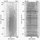
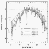
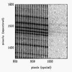
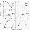
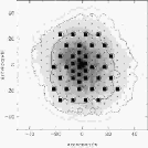
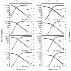
Flat-field exposures of a quartz-lamp illuminated white spot on the dome interior are used to determine the relative fiber throughput and spectrograph vignetting, and to separate these two effects. The full 2-dimensional CCD image of a flat-field exposure for the echelle grating (Figure 1) gives a qualitative sense of low frequency variations present in both spatial and spectral dimensions, and high-frequency (fiber-to-fiber) variations present in the spatial dimension. Figure 2 quantifies the relative throughput as a function of fiber number, normalized for the fibers in the center of the slit (# 38-44), for every setup in Table A1. This plot is derived from the extracted spectra of flat-field images using the IRAF dohydra routine; the values are a mean over the fiber traces. We decompose this spectrograph slit-function into the low-frequency variations due to field-dependence of vignetting within the spectrograph, and the high-frequency variations due to fiber-to-fiber variance in throughput and/or FRD. Detailed results appear in Appendices A and B.

4.1.1 Fiber-to-Fiber Variations

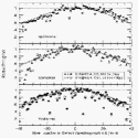
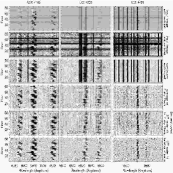
The pattern of fiber-to-fiber throughput variations in Figure 2 are repeatable at different wavelengths and with different gratings at the same wavelength. This is seen for DensePak and the Hydra-red cables as well (Figure 3). The behavior indicates the variations are real, and wavelength-independent.

To understand what causes these variations, uncharacteristically low- and high-throughput SparsePak fibers are marked in Figure 2. Of the 7 fibers which also have reliable laboratory throughput measurements, there is a rough qualitative agreement between their relative throughput. Referring to Figure 13 of Paper I, fibers 1,3,11, and 22 are consistently low in both plots, while fibers 40, 41, 54, and 70 are at or near the mean. Fibers 19, 37, and 74 are also marked as relatively low-throughput fibers. Fiber 37 (and to a lesser extent fibers 3 and 73) have anomalously low relative throughput, but neither fibers 3 nor 37 show signs of anomalous FRD (Figure 16, Paper 1). Differential FRD does not seem to be responsible for low fiber throughput.

Watson et al. (1994) claim similar variations in fiber throughput with a multi-fiber spectrograph (FLAIR II) on the 1.2m UK Schmidt are due to end blemishes. In comparison to SparsePak, DensePak has fewer fibers with anomalously low throughput (for their slit position), but a greater dispersion at a given slit position; the Hydra-red cable has significantly more fibers with anomalously low throughput. We have carefully inspected both ends of the SparsePak fiber cable. We find evidence for blemishes on active fibers, but these do not correlate with fiber-to-fiber variations in the slit-function. Since FRD does not appear to be the culprit and there is no evidence for wavelength-dependence, we can only surmise that these variations are due to blemishes not readily detectable at the fiber surface.

4.1.2 Vignetting and Blaze Functions

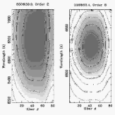
To derive the product of the vignetting and blaze function we remove the high-frequency, fiber-to-fiber variations from the two-dimensional extracted flat-field spectra via a low-order surface fit. This is illustrated for the 860 l/mm grating (2nd order) and the echelle grating (8th order) in Figure 4. Observations of spectrophotometric standards (§4.2) reveal flat-field color-terms are $<$ 3% over 6500-6850Å using the echelle grating, and therefore are likely to be minimal over the slightly broader wavelength range observed with the 860 l/mm grating.

We use these low-frequency maps to calculate the relative mean throughput across the slit, as well as the relative throughput at the slit ends for the central, half- and full-wavelength range limits (columns 13-16, Table A1, Appendix A). Relative vignetting is significant at the edges (up to a factor of two less light). Low-order gratings have superior performance in the spatial dimension compared to the echelle because they are used at smaller camera-grating distance (see below). A more significant performance gain for the low-order gratings is seen in the spectral dimension, largely due to the blaze function. Echelle-grating setups must be optimized carefully for the specific wavelength range of interest.

4.1.3 Geometric Vignetting Model

We have constructed a geometric model of the spectrograph to match the observed slit-function. The model is important because it allows us to place our differential measurements onto an absolute scale. The model uses the known, clear apertures of the optical components, obstructions, their physical layout, and the laboratory-measured mean SparsePak beam profile (Paper I). The low-order curves in Figure 2 represent the models for each of the spectrograph setups; Table A2 in Appendix B summarizes the vignetting for an on-axis (slit center) and off-axis (slit end) fiber at the central wavelength of that setup.

The agreement between data and model is excellent. Spatial vignetting is minimized for the shortest camera-grating distances (d_gc). This subtle behavior is recovered in detail by our model.

Without our model one might naively conclude that vignetting losses (averaged across the slit) are only be 11-18% (column 13 of Table A1). The real throughput loss is much larger, taking into account the on-axis vignetting estimated via the model (column 10, Table A2). We conclude between 44% and 77% of the light is lost through geometric vignetting in the Bench Spectrograph (not including any transmission, reflection, or quantum efficiency losses). Clearly there is room for improvement.

Our model indicates vignetting could be significantly decreased by placing the spectrograph pupil closer to the grating and camera objective, or vice-versa. Currently there is no pupil re-imaging. Gains for the end-fibers (columns 14-16, Table A1 and column 16, Table A2) range from factors of 2 to 4.

4.1.4 FRD Effects

One subtlety which our model does not match is the slight asymmetry of the SparsePak vignetting function in Figure 2 about the slit center (the optical axis). The most likely reason for the asymmetry is due to the larger FRD for smaller fiber numbers, as shown in Figure 16 of Paper I, due to the decreasing radius of curvature in the fiber feed as a function of fiber number. If so, the vignetting profile should become symmetric about the optical axis for Bench fiber feeds using smaller fibers since differential FRD due to foot curvature is likely to be smaller.

To test this hypothesis we have plotted the relative throughput for SparsePak, DensePak, and the Hydra-red cables for two spectrograph configurations in Figure 3. These cables have fiber-diameters of 500 $\mu$ m, 300 $\mu$ m and 200 $\mu$ , respectively. Dome-flats for all cables were measured one after the other with the same spectrograph configuration. Smooth curves are our models for these specific setups using the laboratory-measured SparsePak mean beam profile in all cases.

Low-frequency throughput variations (the slit-function) are different for each cable, but the differences are subtle. For example, the Hydra-red cable, with the smallest (most flexible) fibers shows the most symmetric slit-function of all the cables. This is consistent with our hypothesis. DensePak has the most asymmetric slit-function of all, with extremely low throughput at one end (the top) of the slit. This may indicate the presence of additional stress for the top-end fibers (for example, these fibers are at the edge of the array – see discussion in §6.3 of Paper I), or another source of cable-specific vignetting, e.g., a blockage or improper placement of the fiber slit in the fiber-feed toes.

The similarity of the gross vignetting function in Figure 4 for all cables is consistent with our findings in Paper I that the beam profiles for the various fiber cables are similar. This, coupled with the success of our geometric spectrograph model, indicates the measured beam profiles are correct and our geometric throughput model is accurate.

4.2. Absolute System Throughput

SparsePak’s large fibers enable reliable spectrophotometric calibrations using standard stars. Aperture corrections are relatively small and well-estimable using the near-integral core of the SparsePak object grid. Extended-source spectrophotometric standards exist and have been used with DensePak and Hydra (e.g., NGC 7000 for H $\alpha$ calibrations, or Jupiter for continuum calibrations; C. Anderson, private communication). The advantages of spectrophotometric standard stars are their sky coverage and multi-wavelength calibration. A successful measurement near 6700Å of a stellar spectrophotometric standard allows us to estimate the total system throughput of telescope, fiber cable and spectrograph combined.

4.2.1 Aperture Corrections

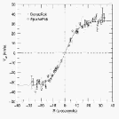
SparsePak aperture corrections are described in Appendix C. These corrections are calibrated as a function of PSF FWHM between 0.45 and 2.5 arcsec based on $R$ -band CCD images taken at the same telescope port. This is suitable for our SparsePak spectrophotometric calibration measurements. The fraction of light enclosed within a central fiber is between 97% and 93% for the lower and upper quartile in currently-delivered image quality at WIYN (0.7 and 1.0 arcsec FWHM, respectively); the median value is 96% at 0.8 arcsec FWHM. Under very poor conditions of 2 arcsec FWHM, the encircled energy is $\sim$ 75%. Based on the ratios of flux in central and ring fibers, we estimate we can determine the 3-25% aperture corrections within 1-2% overall.

4.2.2 Spectrophotometric Observations

A 600 second observation of the spectrophotometric standard Feige 34 (Massey et al. 1988) was made with SparsePak on the night of March 25, 2002 in good conditions at 1.12 airmasses. The spectrograph was configured in order 8 of the echelle grating (Table A1), covering 6500-6850Å. The star was centered on fiber #52, the central fiber within the source grid. Light is detected in this fiber and in the surrounding 6 fibers, with a ratio of $0.0344\pm 0.0003$ for the sum of these 6 fibers relative to fiber #52. The light distribution in the surrounding fibers is azimuthally uniform to $<1$ %, indicating good centering. Based on the results of Appendix C, the derived aperture correction is $11.5\pm 1.5$ %.

4.2.3 Derived Calibration

System throughput is calculated using the effective telescope aperture of 7.986 m² (17.1% central obstruction of the 3.5 m diameter primary by secondary and baffle), and an extinction coefficient of 0.097, appropriate for 6700Å at KPNO. There is a small correction of 2.5 $\pm 0.5$ % to account for light lost in the spectrograph CCD focal plane due to the finite extraction aperture equivalent to $\sim$ 9 unbinned pixels (see §5.2 and §5.3; a comparison of Figures 5 and 9 indicates scattering at 5131Å and 6687Å is comparable). Finally, we converted the throughput estimate from fiber #52 to the on-axis and spatially-off axis (slit-edge) values using the vignetting function defined by dome flats at the central wavelength near 6687Å. In this echelle setup the peak efficiency is slightly redward due to the blaze function. The efficiency on-axis is 94% of peak.

Our results yield a mean efficiency of 4.1% and a peak efficiency of 7.0% from the top of the atmosphere, discounting light lost outside of the fiber in the telescope focal-plane and outside the spectral extraction aperture. Including losses from the atmosphere (1 airmass) and apertures lowers the values to 3.2 and 5.5% for mean and peak, respectively. The mean is over all SparsePak fibers and wavelengths. The uncertainty is of order a few percent of the estimate, with the largest contribution from the extinction correction. The peak efficiency of this echelle configuration compares favorably to the estimate of 5% peak efficiency using the 860 l/mm grating and Hydra cables, quoted in the Hydra Manual. Assuming the relative efficiencies of the gratings are 50% and 65%, respectively, the slight increase in efficiency is significant. Some of this gain may be due to the decreased vignetting from the more open design of the SparsePak toes, the larger SparsePak fibers, and perhaps a more careful treatment of the aperture corrections.

Appendix B presents an estimated throughput budget for SparsePak, spectrograph, telescope plus atmosphere. Our calibration is used to establish the transmission of the spectrograph camera optics. A general discussion is found in the concluding section of the paper.

5. FIBER SPACING, SCATTERED LIGHT, AND OPTIMAL EXTRACTION

5.1. Fiber Spacing

Based on identifying and tracing apertures with high S/N dome flats, we find the fiber spacing to be 10.61 $\pm$ 0.16 pixels at 6600-6700Å (each pixel is 24 $\mu$ m). The spacing uniformity, apparent in Figures 1, 5 and 6 is better than 1.5%. Because the all refractive camera has a chromatic focus dependence, so too does the spectrograph demagnification. We measure a fiber separation of 10.69 pixels at 8675Å, and 10.42 pixels at 5131Å. Given the 902 $\mu$ m outer-diameter of the stainless-steel micro-tubes used to house fibers in the slit, and $\leq$ 0.5-1 $\mu$ m of glue thickness between micro-tubes, we derive the spatial demagnification changes from 3.52 to 3.61 between 8700 and 5100 Å. These values bracket the nominal ratio of the collimator and camera focal-lengths.

5.2. Scattered Light

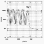
SparsePak’s fiber-to-fiber placement was designed to yield minimum of waste along the slit, but provide sufficient separation to avoid significant cross-talk between fibers in a spectrograph where the coherent internal reflections are small. These attributes are illustrated in Figure 5. Note the faint arc lines continuing to the right of the slit. The curvature and blueward shift of this arc indicates this is a reflected portion of a more inner region of the slit; the reflection deflects the image in the spatial dimension. Since the reflection amplitude is $\sim$ 0.1%, it will not be considered further.

A cross-section of a portion of Figure 1, plotted in Figure 6, shows fibers are well separated relative to the FWHM of their spatial profiles. A low level of signal is present in the trough between fibers ( $\sim$ 2% of peak). The flat-field image was bias-subtracted, so counts are due to photon flux, and represent scattered light. The scattering profile evident in the right-half of Figure 6 appears to be a power-law. We will show this is indeed the case. However, since this profile is a superposition of the profiles from all fibers, it is not possible to determine if the scattering properties of the fibers are uniform. We therefore turn to independent measurements where the fiber light-profiles are individually accessible.

5.2.1 Quantitative Measurement

For quantitative measures of scattering and cross-talk between fibers, we utilize exposures of single bright stars down individual fibers. Exposures were sufficiently short (5 sec at 8650Å and 30 sec at 5125Å) that sky counts are undetected, and hence yield high-contrast, continuum spectra in single fiber channels. While filling factors at the fiber inputs are not the same as for dome-flats, the output far-field pattern – relevant for the estimate of cross-talk from adjacent and more distant fibers – will not depend on these details of the fiber illumination in the telescope focal plane. Some cross-talk in the telescope focal plane is present at very low light levels of 0.1-1% when using fibers within the SparsePak source grid. Despite the large fiber size and separation, this cross-talk is due to the tails of the PSF. Since the 7 sky fibers offer the most isolated fibers in the telescope focal-plane, these were used for our primary measurements.

Figure 7 shows the spatial profiles for the two spectral regions investigated with the echelle grating: 5125Å and 8650Å. Scattering at 5125Å is 10 times lower than at 8650Å for reasons which are currently under investigation. The raw spectra exhibit very low levels of ghosting far away from the exposed fiber at the 0.03% level, but only occur for fibers illuminated near the lower edge of the slit (i.e., high fiber numbers), closest to the semi-reflective surface of the optical bench. There is no discrete scattering detected at a significant level. The spatial cuts of the light profiles in Figure 7 can be characterized well by a Gaussian core going down to 0.04% or 1% of their central intensity, respectively for 5125 Å and 8650 Å followed by a break into a power-law tail.⁵⁵5This is reminiscent of the profiles observed for stellar point-spread-functions observed in direct images, e.g., King (1971). In this case, certainly, the scattering is not coming from the atmosphere, but is coming directly from the optical components within the spectrograph.

5.2.2 Coherence

The spectral signal in the scattered light quickly degrades such that the scattered signal is a smooth continuum devoid of features found in the original spectrum. This appears to occur within 6 pixels away from the central peak. We could check this because our illumination source is a K1 III giant star (HR 4335) with deep, sharp spectral features, e.g., the near-infrared CaII triplet. The degradation in features within the scattered light is due to the fact that the scattering is a two-dimensional process. This is desirable because the cross-talk contributes a featureless continuum that does not introduce high-frequency spectral structure.

5.3. Optimal Extraction

5.3.1 Random vs Systematic Errors

Given the presence of scattered light, it is essential to investigate the trade-offs between different spectral extraction schemes in terms of random versus systematic errors. The considerable literature on this topic (e.g., Marsh 1989, Hynes 2002) mostly focuses on cases not relevant to SparsePak or Bench Spectrograph data. The IRAF dohydra package offers two options which suffice to span the range of viable approaches. The first represents a unweighted spectral extraction within some relative surface-brightness threshold, as defined by the dome-flat trace. The advantage of this algorithm is that it is simple. The second algorithm is a weighted extraction based on the scheme of Horne (1986), designed in the context of long-slit spectra where the weights are defined from the source spectrum itself, suitably smoothed or otherwise averaged. For multi-fiber data, the dome flat is used to define the weights. In the source photon-limited regime, the weighted and unweighted schemes are identical. In our case the “source” is the flux through the fiber. What Horne refers to as the “background-limited regime” is, in our case, the read-noise, or detector limited regime. In the detector-limited regime the weighted extraction has superior S/N, particularly if the extraction aperture is large (i.e. the surface-brightness threshold is low). The relevant issue however, is to weigh the relative gains in total S/N (decreased random error) against the inclusion of additional spurious signal from scattered light (increased systematic error) as the aperture width is increased.

5.3.2 Optimal Threshold

To investigate the trade-offs of random vs systematic errors, we calculate the normalized surface-brightness profile, integral “source” counts, integral “scattered” light, and the integral S/N versus the extraction half-aperture. The latter two integrals are calculated both for weighted and unweighted extraction using the measured surface-brightness profiles of the stars. Measurements were made in the source-limited regime, from which we estimate the S/N profiles for a variety of cases from source-limited to detector-limited regimes.

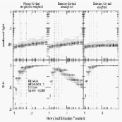
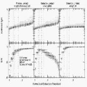
Figures 8 and 9 show the results for the 5125Å and 8650Å spectral regions. Because focus variations exist, the details of these plots depend on the location of the spectrum on the CCD, but is relatively independent of fiber. The Figures show results for two fibers at their central wavelength. One has above-average throughput near the edge of the slit; the other with below-average throughput near the center of the slit. Their behavior is essentially identical.

While the scattering amplitudes are different at 5125Å and 8650Å, at both wavelengths the scattered light contributions to a given fiber continue to be significant for up to 10 fibers distant on either side of the fiber under consideration. Further, the half-light radius (i.e., extraction thresholds of 0.5) defines a nearly optimal extraction. Within this aperture 85-90% of the light is contained, the S/N peaks at this radius in the read-noise-limited regimes, and the scattered light contribution is 0.8% and 10%, respectively for 5150Å and 8659Å. This corresponds to extraction apertures of 4 pixels, considerably smaller than the $\sim$ 10-pixel fiber separation. At lower extraction thresholds (larger extraction apertures) the S/N increases by less than 5%, but only for the source-dominated regime, while the scattered light contribution continues to rise. At higher extraction thresholds (smaller extraction apertures), the scattered-light can be diminished by 20-30% of its value at the half-light radius, but the S/N decreases rapidly.

5.3.3 Weighted vs. Unweighted Extractions

Figures 8 and 9 also shows that the S/N and scattered light profiles are improved for the weighted extraction, but only for the detector-limited case at large extraction apertures, which is uninteresting.

Figures 10 and 11 show a broader picture of the trade-offs between systematic and random error as a function of extraction threshold. In these figures, the integrated scattered light and S/N is plotted as a function of the extraction threshold and position on the detector. The extraction threshold is normalized to the peak intensity of the fiber spatial profile. The lower the threshold, the larger the aperture, as defined in Figures 8 and 9. In Figures 10 and 11, scattered light is calculated to contain contributions from the nearest 10 pairs of neighboring fibers, normalized to the total light from the fiber as determined from large apertures in from the profiles in Figure 7. S/N is normalized by the peak value for the weighted extraction for each of the two regimes: photon-limited and detector-limited. In general, the first and last 20% of the recorded spectrum have larger amounts of scattered light due to degradation in the spatial focus, while the S/N profile is essentially constant. Greater than 95% of peak S/N can be obtained while keeping the total scattered light to $\sim 1$ % of the signal. Over the entire CCD (at all wavelengths), an insignificant improvement can be made by considering a weighted (optimized) extraction.

For these reasons we advocate using an unweighted extraction with a threshold near the half-maximum level.

6. SKY SUBTRACTION

Sky subtraction with fiber-fed spectrographs historically has been a difficult task; the literature is littered with examples. There also is an alarming divergence in the discussion of why fiber-fed spectrographs perform poorly in this regard. However, some work has shown convincingly that a primary contribution to systematic errors in the subtraction of spectrally unresolved sky lines are the field-dependent optical aberrations present in spectrographs (e.g., Barden et al. 1993 for the Mayall 4m RC spectrograph, and, indirectly, Watson et al. 1998 for the 2dF system).

Recent literature begins to address this issue of field-dependent optical aberrations in the context of refined sky-subtraction algorithms, e.g., Viton & Milliard (2002) and Kelson (2003). We concur that the practical difficulty of achieving good sky subtraction for data from fiber-fed spectrographs has been the use of sky spectra far from the source spectra in the spectrograph focal plane. This is something that typically would not be done with multi-slit data. The basic problem with sky subtraction with fiber-fed spectrographs, then, is not the fibers nor the spectrographs they feed, but the way in which the data is processed. Where our argument differs from others is in the nature of solution to the sky-subtraction problem, and its efficiency.

6.1. Inefficiencies in Observational Methods

The frequently-used method for optimizing background-limited observations with fibers is to modify the data-gathering procedure, namely to adopt a beam-switching strategy. In this observing mode each fiber alternates in time between sampling sky and source such that a sky spectrum can be built up out of spectra taken through the same fiber and spectrograph path as the source observations. This has been shown (e.g., Barden et al. 1993) to improve sky-subtraction performance. Nod-and-shuffle (Glazebrook & Bland-Hawthorn, 2001) is a significant technical improvement along these same lines. The advantage of the latter is the time-averaged simultaneous nature of the source and sky sampling, and scanning of the signal over many pixels. A compelling argument for why the dominant source of systematic error with sky subtraction in fiber-fed spectrographs is due to field-dependent spectrograph optical aberrations is that both of these techniques dramatically improve the quality of sky subtraction.

While beam-switching and nod-and-shuffle go a long way to solving the sky-subtraction problem, they incur a significant (50%) efficiency penalty into the data gathering process. Alternatively, a judicious design and allocation of sky fibers within the spectrograph slit, coupled with the proper handling of sky subtraction, should permit shot-noise–limited performance with no penalty in observing efficiency for a wide variety of programs. Instead of a solution involving an inefficient data acquisition strategy, we have found a less wasteful solution using a better instrument design and approach to data processing.

6.2. A New Sky Subtraction Algorithm

We consider here the problem of subtracting night sky lines and continuum where the source signal of interest consists of narrow emission lines. Our solution works equally well for source signals consisting of well-separated narrow absorption lines. The broader issue of subtracting night sky lines from data where the source signal consists of broad or blended absorption lines is deferred to future papers.

There are a number of software packages available for reducing multi-fiber data, but we focus on IRAF’s dohydra routine and SparsePak data to illustrate the problem and solution. The dohydra routine is a complex script calling several independent tasks which serve to identify on each CCD frame the multi-fiber apertures, trace them in the spectral dimension, extract an optimally weighted spectrum for each fiber for matching source, flat, and wavelength-calibration frames, and finally, gain-correct, wavelength calibrate and rectify the source spectra. At this tertiary stage, the sky spectra can be identified, combined, and subtracted from the individual source spectra. Herein lies the key issue.

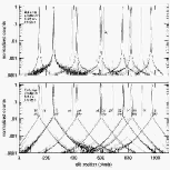
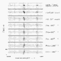
The basic problem in sky subtraction arises when the fiber data is not treated like long-slit or multi-slit data, despite the fact that fibers are typically fed into a spectrograph in a pseudo long-slit. Because the optical transfer function (OTF) varies over spectrograph field angles, the width and shape of spectrally unresolved lines changes along the (pseudo-)slit. This is illustrated in Figures 12 and 13, which demonstrates the pitfall of using all of the sky fibers to define a mean sky spectrum. While this example uses Thorium-Argon line-lamp spectra, this high S/N data of uniformly distributed, unresolved lines make the point about the performance of subtraction of strong sky-lines: It is the high-frequency spectral information that is the dominant problem – i.e., the sky-lines, not the continuum. It is these unresolved sources whose profiles change as a function of field-angle within the spectrograph. For this reason one would like to have sky fibers placed evenly along the slit, and indeed this was one of the criteria in our mapping of fibers from the telescope to spectrograph focal planes (see Paper 1). In this situation, one can assign a sky fiber or the proper interpolant to each source fiber. Unfortunately, such a simple algorithm introduces significant shot-noise since, for any given source, fewer fibers are being used to measure sky.

The solution is to use the fact that the variation in the OTF is a low order function of slit position, and is usually symmetric about the optical axis. All of the sky fibers can be used in concert to constrain a low-order function for the spatial modulation of the sky level at each spectral channel (wavelength), in a mode similar to what is done typically for sky subtraction with long-slit spectra. If the spectral features of interest do not occur at the same wavelength in each fiber, then many fibers can be used to fit the “sky” at any particular wavelength. This greatly increases the signal-to-noise of the sky estimation.

The sky subtraction method we propose takes advantage of situations where emission lines of interest (i) only occur in a limited number of spectra or (ii) occur at different wavelengths in different spatial channels (henceforth fibers) due either to kinematic sub-structure in the object or a range of radial velocities in multiple objects. In case (ii), the fiber-to-fiber change in wavelength of the emission feature should be larger than the line-width. A prerequisite is that the continuum levels (sky plus object) have been removed and the spectra are all wavelength calibrated and rectified to the same dispersion relation. Consequently, the spectra should only contain high-frequency spectral features (emission or absorption lines from sky and object).

A synopsis of the specific sky-subtraction algorithm we propose is this: (1) rectified fiber spectra are put into a spatially sorted, two-dimensional format; (2) spectral continuum is subtracted (sky and source) via low-order polynomial fits to each fiber channel; (3) sky lines are subtracted using a suitable, clipped mean; (4) continuum is replaced; and (5) line-subtracted sky fibers are used to subtract sky continuum from source fibers. The most complicated step is the removal of the sky lines (3). The detailed algorithm is found in Appendix D.

6.3. Algorithm Performance

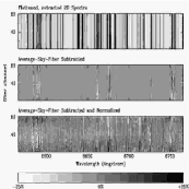
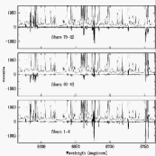
The first three steps are illustrated in Figure 14 for three sources carefully chosen to have emission features on strong sky lines, but with a range of internal-velocity spreads. (The last two steps are only necessary to provide continuum information for, e.g., determining line equivalent-widths.) For comparison, we have shown three implementations of step 3, including (i) a straight mean of the seven sky fibers (fitting a zeroth-order baseline; this is method 3a in Appendix D); (ii) a second-order fit to the seven sky-fibers, with no clipping; and (iii) a second-order fit to all 82 fibers, with an interactive-clipping of fibers (this is method 3c in Appendix D). A visual inspection shows the latter implementation is significantly superior in terms of random error.

This preferred algorithm (Appendix D, item 3[c]: “iterative clipping using a wavelength-dependent noise estimate”) works in the regime when the majority of fibers have source features that are separated from each other by more than the sources’ line-width. For redshift surveys and high-spectral resolution kinematic studies, this regime is usually achieved. (See UGC 7169 and 4256 in Figure 14 as two examples of the latter.) In this case there are significant decreases in random noise by using all of the fibers and there is no need to assign any fibers to sky.

When should the algorithm fail? Consider the following two types of observations: (a) An extended source with no velocity structure or N sources at the same radial velocity within the spectral resolution. This fails because all of the source features are aligned in wavelength – like the sky. UGC 4499 is a good example of this case, and indeed a close inspection of the spectrum for UGC 4499 in Figure 14 reveals a systematic over-subtraction at the bright H $\alpha$ line which straddles a bright sky-line. (b) An extended source with spatially-resolved velocity structure comparable to the (unresolved) velocity width for each fiber. This will systematically over or underestimate the sky level (emission and absorption lines respectively) and hence modify the profile shapes.

When only a restricted set of the “sky” fibers can be used to estimate the night-sky line emission, as is the case for UGC 4499 in Figure 14, a straight average of all sky fibers appears to yield a result superior to fitting a 2nd-order function to these restricted channels. This is true even though the sky-fiber locations are chosen carefully to span the spectrograph slit. The 5th panel from the top in Figure 14 reveals spatial curvature in the sky-subtracted continuum which is not seen in the 4th panel. The poorer result of using a low-order polynomial as an interpolant stems from having insufficient points to constrain the fit, hence resulting in a noisy fit.

In summary, we find the sky-subtraction performance of multi-fiber spectra using dohydra’s algorithm with SparsePak’s sky-fiber slit-mapping geometry is, to first-order, as good as long-slit data. Under certain conditions, this simple algorithm can be replaced with a more aggressive procedure which yields superior performance. This scheme also can be applied to long-slit data provided certain conditions are met on the spatial and spectral distribution of source emission.

6.4. Discussion

Four ancillary conclusions stem from the above analysis:

1. The above result concerning the poor, second-order fits to seven sky-fibers modifies the arguments made by Wyse & Gilmore (1992) and by us (Paper I) on the optimal number of sky fibers. Specifically, the optimum number is probably larger than the analytic formulae cited in these references. Before designing future fiber systems, the optimum number of sky fibers should be explored in the context of the sky-subtraction algorithm presented here.

2. Figures 12 and 13 do not reveal significant fiber-to-fiber differences in line profiles. There are no apparent high–frequency variations superimposed on the smoothly-changing mean profile shape across the slit. This indicates that beam-switching or nod-and-shuffle will not significantly improve the sky-subtraction performance beyond the algorithm outlined here, and would increase random errors for an equal amount of observing time.

3. Our proposed algorithm cannot be applied to multi-slit data in its current form because slitlets are typically offset in both spatial and spectral dimensions. Similar wavelengths in different slitlets are subject to discontinuous ranges of optical aberrations. Hence while fibers introduce entropy losses via FRD, the ability to use fibers as light-pipes to remap focal planes may have significant advantages for efficient, high-performance sky subtraction.

4. The result that the straight average of the sky fibers does a good job for SparsePak sky-subtraction (e.g., Figure 14) is surprising. Perhaps the spectrally-unresolved lines are still well-sampled in the spectral direction due to the large fiber size; the shape of the spectrally-unresolved lines are dominated by the demagnified fiber image, and not the field-dependent OTF. However, one must reconcile the apparent lack of residual structure seen for real on-sky spectra (Figure 14, 4th panel) with what is seen for Thorium-Argon calibration-lamp spectra (Figures 12 and 13).

One possibility is that the results of Figures 12 and 13 are not representative of “on-sky” data. It is not known, for example, if the illumination of the calibration lamps onto the fibers is the same as the sky and source illumination, nor if this lamp illumination is constant across the fiber array. However, since the residual pattern seen in the lamp spectra are continuous across the slit, while the mapping from the telescope to spectrograph focal plans is not, it is hard to imagine that this explanation is valid.

Another possibility is that the $<$ 25% residuals seen in Figures 12 and 13 occur primarily at low levels in, i.e. the wings of, emission-lines. Hence the corresponding features in the on-sky data of Figure 14 are difficult to detect because they are below the level of the random noise. Indeed the panel 4th from the top does show low-levels of spatial variation in the sky-line residuals. Therefore we believe it is warranted to dismiss our concerns about differences of illumination. Our conjecture remains plausible that SparsePak’s large fibers yield relatively invariant resolution elements, thereby simplifying sky-subtraction.

7. EXAMPLES OF COMMISSIONING SCIENCE

A hall-mark of SparsePak IFS is the ability to achieve spectral resolutions $\sim$ 10,000, work at low surface-brightness, and create kinematic or spectrophotometric maps that can be registered reliably to imaging data. SparsePak resolution and sensitivity limits enable the study of gas and stellar kinematics in otherwise unfavorable geometric projections, such as face-on disks, and create the ability to probe velocity dispersions in these dynamically cold systems. Spatial registration of kinematic and photometric properties is critical for deriving dynamical information. Illustrative examples are given below.

7.1. Velocity-Fields at Echelle Resolutions

Andersen’s (2001) study of the photometric and kinematic properties of face-on disks showed that optical, bi-dimensional spectroscopy with DensePak (Barden et al. 1998) yields efficient determinations of kinematic inclinations for nearly face-on systems – in an inclination regime that has been claimed unmeasurable with radio-synthesis observations. The precision of these measurements enables, for example, a Tully-Fisher relation to be measured for galaxies with inclinations between 15 and 35 degrees (Andersen & Bershady 2002, 2003). While these studies focused primarily on “normal” disks with Freeman-like central surface-brightness, several sources approach the low-surface-brightness (LSB) regime. One such source is PGC 56010. Re-observation with SparsePak reveals the relative merits of this array compared to DensePak.

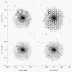
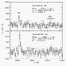
The pointing maps for PGC 56010 in Figure 15 show SparsePak signal detection is much more extensive and complete than for DensePak. Both arrays were used for the same amount of time and in comparable (good) conditions. Further quantification is derived from the line profiles for a single fiber from each array, taken to lie near the same position (Figure 16). The measured H $\alpha$ flux ratio is 3.34 (SparsePak/DensePak), higher than the expected ratio of 2.78, based on fiber sizes and assuming a uniform surface-brightness source. The enhanced SparsePak performance is comparable to the gains noted in §4.2, possibly due to the decreased vignetting in the SparsePak fiber toes.

We also compared the radial light-profile of the spectral continuum for this source, measured using both arrays. These profiles, rendered in units of detected electron per hour per fiber, should be offset by the factor of their relative area and throughput. The comparison does not require any two fibers to be spatially coincident, and yields a scaling consistent with our emission-line measurement.

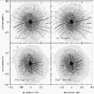
The net effect of the enhanced SparsePak etendue is seen in Figures 15 and 17: The velocity field, derived rotation curve and estimate of disk inclination are significantly improved using SparsePak. This success has lead to further study of LSB systems with SparsePak (Swaters et al. 2003).

Despite SparsePak’s sparse sampling, the fiber-packing geometry still enables the spectra to be sorted for quick assessment of the radial extent and spectral coherence of the emission-line data, as described in Appendix E. Such sorting is invaluable for assessing the data quality at the telescope, or for quickly estimating kinematic position angles of barred spirals (e.g., Courteau et al. 2003).

7.1.1 Absorption-line vs. emission-line velocity fields

The velocity fields of disks traced by stars and ionized gas can have systematic differences due to the fact that the gas is collisional while stars are not. SparsePak can probe these differences even in nearly face on systems. NGC 3982 serves as an example, chosen for its size, high surface-brightness, and extensive existing data (Verheijen 1996). SparsePak footprints for observations in the H $\alpha$ and CaII triplet spectral regions are shown in Figure 18.

Because the stellar absorption-line observations were only sparsely sampled, we used the H $\alpha$ data to explore sampling effects on the derived velocity field. We find the basic shape and position angle remains unchanged over a factor of three range in sampling (Figure 19). We also find the stellar and gaseous velocity fields are similar, with nearly identical kinematic PAs, as expected if the gas and stars are co-planar. However, there is less curvature of the stellar absorption-line iso-velocity contours. This is evidence for asymmetric drift, which we quantify elsewhere.

7.2. Absorption-line Velocity Dispersions at Echelle Resolutions

As part of the primary SparsePak commissioning science, we undertook a pilot survey to measure the stellar kinematics of nearly face-on spiral disks to directly estimate their mass from the amplitude of the vertical stellar velocity dispersions (Bershady et al. 2002; Verheijen et al. 2003, 2004). This survey consists of SparsePak H $\alpha$ observations of several dozen galaxies of suitable size and apparent inclination; MgI and CaII-triplet observations of a kinematically regular and suitably inclined subsample; and MgI and CaII-triplet observations in identical configurations for a library of several dozen template stars for cross-correlation. In our initial commissioning run we explored the viability of the high-resolution order-7 echelle setup for the CaII triplet, which achieves $\lambda/\Delta\lambda\sim 24,000$ . In the remainder of §7, we evaluate data taken with this configuration by comparing them to similar observations taken on a subsequent run using the lower-resolution, but higher throughput order-6 echelle setup and order 11 setup for the MgI region.

7.2.1 Resolution Performance From Stellar Line Profiles

We have explored two observational modes for acquiring a spectral library for application to extended sources. Stars were observed in “stare” mode and by drifting them across a row of fibers. For “drift” mode, the illumination typically was uniform to about 15% for 16 fibers. Because of azimuthal scrambling, drifting stars across the fiber faces (i) samples all of the fiber modes, and (ii) yields a time-averaged fiber image which more closely approximates the near-uniform fiber illumination of extended sources, e.g., galaxies. A priori, we thought such drifting was important to minimize slit-illumination systematics in cross-correlation analysis of stellar templates with galaxy spectra. However, our preliminary inspection has not revealed significant systematic differences in line-width or shape between stellar spectra obtained in “stare” or “drift” modes.

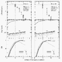
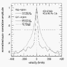
Observations of a K-giant, shown in Figure 20, illustrate one of the advantages of the MgI region. In the order 6 and 7 spectra the CaII-triplet lines dominate over a number of other weaker, but narrower lines (primarily from Fe I). The intrinsic widths, $\sigma$ , of the CaII triplet are 15-35 km s^-1 in the high resolution spectrum, and 27-43 km s^-1 in the lower-resolution spectrum, where the width correlates with the line-strength. The MgI lines in order 11 have comparable $\sigma$ ’s between 25 and 35 km s^-1, but the spectrum in this region is filled with strong, narrow lines. These narrow (mostly iron) lines have $\sigma$ ’s of 7-8 km s^-1 (about 4 pixels) in the high resolution spectrum, and are nearly unresolved.

An auto-correlation analysis of these spectra, shown in Figure 21, reveals a significantly narrower peak with $\sigma=13.5$ km s^-1 in the MgI region, compared to 31.5 and 34.5 km s^-1 in the high- and low-resolution CaII triplet region spectra, respectively. The higher-resolution CaII cross-correlation spectrum has a narrower core than the lower resolution spectrum, but no narrower than then MgI spectrum. Hence, despite the strength of the CaII triplet lines, their large intrinsic width, coupled with a paucity of narrower lines, makes this region less attractive than the MgI region for kinematic analysis of systems with intrinsically small velocity dispersions.

7.2.2 Galaxy Spectra and Sky Line Emission in the Red

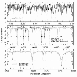
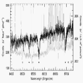
One advantage of high spectral resolution is the ability to separate the plague of emission lines dominating the sky background redward of 650 nm. Spectra in Figure 22, corresponding to 1 hour of integration in the high-resolution, order-7 configuration for the CaII triplet, illustrates the situation. The galaxy spectrum is from a region close to the center of NGC 3982, sampled by fiber #52. The sky spectrum is an average over 6 sky fibers from the same exposure (the seventh sky fiber was contaminated by a faint star). A comparison of the sky spectrum with Dressler’s (1984) seminal paper on the use of the CaII triplet for galaxy kinematic studies reveals an entirely new background terrain at spectral resolutions of 24,000. Despite the remarkable resolution of the sky’s molecular bands and atomic doublets, it is clear that judicious choice of source redshift is required to keep the CaII triplet lines at 8498, 8542, and 8662 Å free of the sky’s strong-lined regions.

7.3. Source Registration and Continuum Calibration

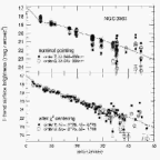
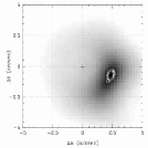
Based on an analysis of the spatial distribution of NGC 3982’s spectral continuum relative to the $I$ -band light profile from Verheijen (1996), we estimate the spectrum of fiber #52 in Figure 20 is centered 2.25 arcsec east and 0.75 arcsec south of the optical center. Similar offsets were found for the order-6 data. The high quality of the $\chi^{2}$ -minimization of a SparsePak spectral continuum map to the $I$ -band surface-brightness, shown in Figures 23 and 24, yields an offset precision of under 0.25 arcsec, and an $I$ -band surface-brightness of 17.75 mag arcsec^-2 for fiber #52’s observed continuum in order 7.

Another registration method we have developed convolves the fiber beam with a CCD image to generate a broad-band continuum map that can be directly compared with the fiber spectral data, fiber-by-fiber. For intrinsically axisymmetric systems suffering contamination from, e.g., foreground stars, the one-dimensional approach used here may have advantages; azimuthal averaging provides filtering for the foreground source contamination. The two-dimensional method is better equipped to register data for more irregular sources, and has been used effectively with low-surface-brightness galaxies, e.g., DDO 39 (Swaters et al. 2003).

7.4. Overall Performance

The above calibration permits several useful calculations. First, based on the order-7 data, the sky continuum in the 848-868 nm region is roughly 18.2 mag arcsec² near full-moon (based on the CCD calibration of the spectral continuum); the total sky background (continuum plus lines) is about 0.4 mag brighter still. (A separate pointing, offset by roughly 26 arcmin to a blank region of sky, but taken immediately following the on-target exposure, yields the same continuum background levels.) In dark time, based on the order-6 data in the 845-884 nm region, the sky continuum drops to 19.6 to 20.2 mag arcsec²; the total sky background is roughly 18.7 mag arcsec².⁶⁶6Estimated sky levels appear 1.2 to 1.4 mag brighter than typical $I$ -band sky backgrounds in full and new moon, respectively. This is partly because we observe redward of the nominal $I$ -band, where the sky background is significantly brighter. We estimate band-pass effects amount to 0.5 and 0.2 mag in the wavelength regions sampled in orders 6 and 7, respectively (Turnrose 1974). Some additional background is due to large zenith distances of 25^∘ and 42^∘, respectively, for order 6 and 7 observations. Massey & Foltz (2000) find between 0.3 and 0.5 mag brightening at Kitt Peak in the $V$ -band at zenith distances of $\sim$ 60^∘ degrees. Assuming more brightening occurs at longer wavelengths (OH gets stronger), this leaves less than a factor of 2 in increased sky-brightness in our observations unexplained, with the worst case being our bright-time observations. Moon illumination was 100% for order-7 observations, but the moon-source distance was over 70^∘. However, it is possible that scattered light off the dome floor, etc., is a cause of the high observed continuum background levels. These values can be compared to the normal-disk central surface-brightness of 20.2 mag arcsec^-2 in the $I$ -band for a galaxy of this color. Hence even in dark-time galaxy disks lie below the sky continuum in the red.

Second, despite the high background continuum level in the order-7 data, within the 4-pixel, unbinned optimum extraction aperture, the sky spectrum is 1:1 photon-to-detector noise-limited (i.e., photon shot-noise is equivalent to the detector read-noise). This can be improved with on-chip binning of pixels, and increased exposure time. On this basis, we estimate the photon and detector noise contributions during dark-time for several setups assuming a $2\times 1$ pixel binning in the spatial direction and a limiting exposure time of 1 hour. (The spatial binning yields no loss of spectral information or beam separation; longer exposures suffer from too many cosmic rays.) Our calculation takes into account the relative dispersion and spectrograph throughput (Tables A1 and A2), CCD quantum efficiency, and sky brightness (19.9 mag arcsec^-2 in the $I$ band and 21.8 mag arcsec^-2 in the $V$ band). Of the two CaII-triplet region setups, the higher-resolution order 7 setup remains 1:1 photon-to-detector noise-limited, while the lower resolution (order 6) setup has a ratio of 1.8:1, i.e., the photon shot noise is almost twice as large as the detector read-noise. In the MgI-setup, at an intermediate resolution and improved ( $\times 1.7$ ) CCD quantum efficiency, but darker sky, the ratio is also 1:1. System throughput increases or improved detector read-noise of at least a factor of 2 are needed to significantly alter this situation.

Third, these data provide an additional check on the throughput of the system, which we estimate is 1.2% from the top of the telescope for fiber #52. This result is in close agreement with our throughput estimates at 6700Å described in §4.2 by taking into account (1) the relative CCD quantum efficiency at 6700Å and 8600Å (0.80:0.47); (2) the relative on-axis vignetting in respective order 8 and 7 setups (0.69:0.41), based on the laboratory-measured SparsePak fiber exit-beam profile summarized in Table 2; (3) the relative grating efficiencies used off-blaze, (we estimate a 10% relative difference between order 8.41 versus order 6.53 with a standard echelle grating 5.5 degrees off-Littrow); and (4) the loss from scattered light (15%, cf Figures 8 and 9).

With this information in hand, we estimate the exposure time required to achieve a usable S/N for measuring absorption line-widths in a “normal” disk ( $\mu_{0}(I)=20.2$ mag arcsec^-2) at a radius of 2.2h_R. This radius is where the rotation curve is usually fairly flat (little asymmetric drift) and the maximum disk circular speed is achieved (Sackett 1997). We adopt S/N = 15 per resolution element as a practical limit for measuring reliable line-widths. We assume 12 fibers are averaged within a radial bin⁷⁷7A galaxy with a scale-length between 10 and 20 arcsec will have between 6 to 18 fibers sampling annulus at R/h_R = 2.2., and each fiber has been corrected for projection. Nearly face-on galaxies are advantageous here, but in general high S/N velocity-fields from ionized-gas emission-lines can be used to deproject the stellar velocity field if the asymmetric drift is zero or otherwise understood.

The NGC 3982 spectrum in Figure 22 has an apparent continuum S/N of 19.6 per resolution element (2.5 pixels), but the true S/N is actually somewhat smaller ( $\sim$ 16) due to the presence of correlated noise in this wavelength-rectified (i.e., re-sampled) spectrum. The latter value agrees with a first-principles calculation of the expected signal-to-noise based on the photon shot-noise (object plus sky) and detector read-noise. Again assuming the same observing conditions as in the previous calculation of photon-to-detector noise ratios we estimate 7, 48, and 10.5 hours of total integration are required in orders 6, 7, and 11 respectively.

The numbers presented in this sub-section in isolation indicate the order-6 CaII-triplet setup yields superior performance for measurement of stellar kinematics in extended, low-surface-brightness systems, while the higher-resolution order-7 setup is suitable only for the highest surface-brightness systems. However, the order-11 MgI setup has lower sky-continuum levels and little contamination from strong sky-lines, $10\times$ -lower scattered light, intrinsically narrower lines, higher instrumental resolution than the order 6 setup, and [OIII] $\lambda$ 5007 for estimating the projected velocities. On balance, and despite the limited band-width of the Bench Spectrograph’s sampling of this order, the MgI region likely provides a superior region for stellar kinematic work with SparsePak.

8. SUMMARY

We have presented the capabilities of SparsePak and the WIYN Bench Spectrograph in several configurations relevant for the study of galaxy kinematics, established procedures for conducting precision spectrophotometry of extended sources, and quantified and understood the throughput efficiency of the Bench Spectrograph. We have used SparsePak to implement significantly improved methods for sky subtraction. In this regard, performance for this fiber-fed system is comparable to long-slit, imaging-spectroscopic instruments. Finally, we have demonstrated SparsePak’s on-sky capabilities based on observations of two, nearly face-on galaxies. Here we summarize each of these components.

The Bench Spectrograph offers a wide range of possible spectral resolutions across the visible band-pass, with trade-offs between resolution and system efficiency. We have focused on the high-end of the resolution range achievable with SparsePak: $\Delta\lambda/\lambda\geq 5000$ . Resolutions between 9,700 and 12,000 are typical with the echelle grating for wavelength between 500-900nm. Resolutions as high as 20,000-24,0000 are possible using the echelle in off-order (high incidence-angle) configurations. These modes are 50% less efficient due to overfilling the grating and lower diffraction efficiency. Gain factors in resolution roughly equal loss factors in throughput. Resolutions of 4,000-6,000 are possible with 2nd-order gratings. Due to the smaller camera-grating distances used for the low-order gratings, made possible by larger camera-collimator angles, off-axis vignetting is $\sim$ 20% smaller than for typical echelle configurations. This, combined with higher diffraction efficiencies make the low-order grating configuration the most efficient, but at the price of lower spectral resolution. The above resolutions are specific to SparsePak, but the trade-offs between spectral resolution and signal-to-noise are generic for the spectrograph.

In all cases we have explored, the spectral sampling is only 2.5-3.5 pixels (FWHM) even with SparsePak’s large fiber diameters due to the large geometric and anamorphic demagnifications in the spectrograph. Spatial sampling is $\sim$ 4 pixels (FWHM). The fiber spacing (roughly 10 pixels) is such that on-chip binning by a factor of 2 can be used in this dimension without signal degradation. This is useful for low-light-level applications where detector noise is significant.

The combined absolute throughput of the telescope, SparsePak and spectrograph has been established, based on measurements of a spectrophotometric standard star, to be 7% peak at 670nm, and 4% mean (over all used field angles – fibers and wavelengths). Our ability to measure reliably the absolute throughput is due to SparsePak’s large fibers and array geometry. Large fibers result in small slit-losses for observations of stellar spectrophotometric standards. The two-dimensional format of the array has allowed us to develop a second-order, empirical formulation of aperture corrections with a precision better than 2%.

The modest system throughput stems in part from the exhibited, strong spatial vignetting function. We have well-matched this vignetting function with a geometric model that traces a realistic (laboratory-measured) fiber-output beam-profile through the optical system. On this basis we have been able to conclude (a) the vignetting is due to the lack of proper pupil placement within the spectrograph and large distances between collimator, grating and camera; and (b) averaged over all fibers, typically half of the light within the spectrograph is lost to vignetting at the central wavelength.

It is remarkable to ponder where the photons are lost overall. A detailed breakdown is documented, and plausibly understood. The fiber introduce only a 20% loss, and are a minor contributor to the overall budget. By our estimate, half of the light is lost before it gets to the spectrograph (“top end” losses due to atmosphere, 3 aluminum surfaces, and fiber surface losses and internal attenuation); half of this light is lost in geometric vignetting within the spectrograph (above); another factor of $\sim 2$ decrease comes from filters and gratings; and a final factor of $\sim 2$ decrease comes from surface-losses on spectrograph optics, dewar window, and CCD quantum efficiency. We have grouped these losses together in this way purposefully. There is little that can be done to any single component in the first and last groupings to significantly increase the throughput; attention to improving many components is needed to make appreciable gains. In contrast, the middle two groupings offer the possibility of making significant throughput gains by shortening the collimator focal-length, properly placing the pupil (see Paper I), and introducing more efficient gratings (e.g., volume-phase holographic gratings, for which order-blocking filters are generally not needed). While collimator changes may result in decreased spectral resolution, the amplitude of the decrease would likely be of order or less than 30%, which would still be sufficient for galaxy kinematic studies. Since photon starvation is the critical limit, the trade of efficiency for spectral resolution is desirable. A program to improve spectrograph throughput along these lines is underway and will be reported elsewhere.

We have also explored the implications of the fiber spacing for scattered light and optimal extraction of the spectral signal. The fibers are regularly spaced and sufficiently well separated for a clean beam extraction, with some degradation in the far red, CaII-triplet region at 860nm. At bluer wavelengths, cross-talk is below 1% when using extraction apertures capturing $\sim$ 90% of the desired signal. At 860nm, the cross-talk rises to $\sim$ 10% for the same captured signal. For SparsePak data, we find that weighted extractions offer little gain over an unweighted extraction, and therefore we advocate the unweighted extraction. An extraction threshold near 50% the peak is optimum.

One of the most striking results from the present work is the quality of the sky subtraction with the SparsePak array. This is due partly to the even placement of the sky fibers along the SparsePak slit, and possibly because the large fibers are well resolved and their monochromatic images are not dominated by the spectrograph OTF. Also important is our development of a new algorithm for data handling and fitting of the sky-fibers. The algorithm includes subtraction of spectral continuum and sky line-emission in separate stages. In the highest-performance implementation of this algorithm, a low-order function is fit to all fibers in each spectral channel to model the effects of field-dependent optical aberrations. By including an interactive clipping algorithm to remove source flux, we have shown that in certain cases almost all of the fibers can be used for sky subtraction, resulting in significant improvement in the S/N of the data. These cases include any situation where discrete source emission in the fibers has a large range of apparent Doppler shifts, e.g., in redshift surveys or galaxy kinematic studies where the spread of internal velocities is large. Here the performance appears to be as good as one might expect from beam-switching or nod-and-shuffle, but our method is twice as efficient.

Two other significant implications stem from our results on sky subtraction. First, there is a need to revisit the optimum number of sky fibers for survey work. We conclude more sky-fibers are needed than traditionally calculated from simple random-error analysis models because such analyses do not consider the effects of field-dependent optical aberrations. This is a critical issue for subtracting unresolved sky-lines. Second, we have realized the advantage of fiber-fed spectrograph over slitlet systems for “multi-object” spectroscopy. The ability of the former to control the mapping of the telescope to spectrograph focal-planes allows for better – or at least more efficient – control over optical aberrations for sky-subtraction purposes. In a very general sense, this offsets the information loss introduced by FRD in the design and use of a spectrograph.

We have also given several examples of the types of science for which SparsePak was designed. We have shown SparsePak easily generates data yielding high-resolution emission-line and stellar absorption-line velocity fields of nearly face-on galaxies. It appears SparsePak has a higher throughput than DensePak by about 20% – above and beyond the 3 $\times$ gains from increased fiber solid-angle. A simple tool can be used to examine such SparsePak data and quickly assess, by eye, the kinematic position-angle of a galaxy. SparsePak’s sampling geometry also permits the a posteriori registration of spectral data to normal CCD images via analysis of the spatial distribution of the spectral continuum. The precision of this registration is better than one-tenth the fiber diameter.

Our primary motivation for building SparsePak, a large-etendue, two-dimensional fiber array, capable of achieving resolutions ( $\sigma$ ) of 10 km s^-1 or better, is to measure the stellar motions and velocity dispersions in galaxy disks. An analysis of kinematic data of a K giant star and the high-surface brightness blue galaxy (NGC 3982) indicates that this is indeed feasible. To measure stellar velocity dispersions at radii of 2-3 disk scale-lengths in a “normal” disk requires $\sim 10$ hours. Given the paucity of such data, even these lengthy integrations will yield important results worthy of the effort. Bench Spectrograph throughput improvements will enable large-scale surveys. Due to the combination of larger intrinsic line-widths, higher backgrounds, and greater scattered light in the CaII-triplet region, we conclude the MgI region is preferable for stellar kinematic studies. For emission-line galaxies the MgI regions also offers the [OIII] $\lambda$ 5007 line within the same spectral window. Therefore in one setting it is possible to trace stellar and gaseous velocity fields, and hence the asymmetric drift, as well as line-of-sight velocity dispersions. Such measurements offer great opportunities for studying the dynamics and mass distributions of spiral galaxies.

SparsePak is now a facility instrument available to the public on the WIYN telescope. A web page on this instrument is maintained at:
http://www.astro.wisc.edu/ $\sim$ mab/research/SparsePak/.

We wish to thank C. Corson, D. Bucholtz, S. Buckley, and G. Jacoby for making SparsePak a reality at WIYN; D. Harmer and C. Harmer for frequent, expert assistance with the Bench Spectrograph and consultation on the optical model; and the anonymous referee for constructive comments. We also thank J. Hoessel and A. Glenn for allowing us to use WIYN Mini-Mosaic data in advance of publication. Support for this project is from NSF AST/ATI-9618849, AST-9970780, AST-0307417 and the UW Grad School.

Appendix A A. SPECTROGRAPH CONFIGURATIONS AND CHARACTERISTICS WITH SPARSEPAK

Table A1 summarizes the spectral and spatial sampling, resolution, and vignetting properties for all setups discussed in this paper. A dewar-azimuth angle of -0.128^∘ was used for all configurations associated with reported measurements. Columns 2-5 list the physical configuration parameters (standard order-blocking filters are not included). Columns 6-12 describe spectral resolution characteristics (§3). Expected spectral demagnification and re-imaged monochromatic fiber diameter are given in columns 6 and 7, based on the geometric properties of the spectrograph. Measured central wavelength, wavelength range, dispersion, sampling (FWHM), and derived spectral resolution are in columns 8-12, based on line-lamp exposures. Dispersions are calculated via line-fitting in dohydra, yielding high precision measurements typically better than one part in 10^-4. Tabulated values for FWHM and spectral resolution are for the central fiber at the central wavelength. “Errors” on the dispersion, FWHM and spectral resolution map the range on these values across the detector. Columns 13-16 describe vignetting characteristics (§4), measured from dome-flat exposures. The measured relative throughput in Column 14 can be directly compared to the modeled vignetting ratio in Column 16 of Table A2 in Appendix B.

Appendix B B. SYSTEM THROUGHPUT BUDGET

Table A2 presents a break-down of the geometric vignetting produced by different optical components, as estimated via our model described in §4.1.3. Columns 1-5 are repeated from Table A1 for reference. Columns 6-16 contain the model vignetting values used to estimate the throughput budget of the spectrograph. The model contains no vignetting from the toes and filter (appropriate for SparsePak but not the other fiber feeds), and no vignetting from the camera enclosure, which should be minimal or non-existent for the camera back-distance used in these setups.

Table A3 itemizes a complete throughput budget for the WIYN Bench Spectrograph and SparsePak cable, starting from the top of the atmosphere, and compared to observations described in §4.2. The spectrograph configuration is for the echelle, order 8, as listed in Table A1, using the X19 interference filter. The “On Axis” budget corresponds to the spectrograph optical axis and central fiber while “Off Axis” refers to the spectrograph light-path for the slit-edge fiber.

Notes to Table A3 document the source of each estimate. Components we have measured directly, and with high confidence, are given a rating of “Excellent”; older measurements we did not make but reported in the Hydra Manual are given a rating of “Good.” One exception is the grating response, where the estimate quality is designated “Fair” because the Hydra Manual does not report a measured value for the actual Bench Spectrograph echelle. Estimates of aluminum reflectance are given a “Fair” rating because actual measurements are not available. Camera throughput (T_cam) is given a “Poor” rating because there is no available information on laboratory measurements or manufacturer specifications on coatings. We have used the measured throughput to derive T_cam in row 20. Given the number of optical elements, the derived value of $\sim$ 75% is reasonable. T_cam values for on- and off-axis agree to within 5% – a confirmation that our geometric model is accurate to within this margin.

Appendix C C. WIYN POINT-SPREAD-FUNCTIONS AND SPARSEPAK APERTURE CORRECTIONS

The stellar profiles observed on the WIYN telescope’s Nasmyth imaging port were analyzed to establish aperture corrections suitable for spectrophotometric calibration of SparsePak data using stellar standards. The imaging port has no corrector, and is used by SparsePak, DensePak, the Mini-Mosaic Camera, and the WIYN Tip-Tilt Module. SparsePak is suited for spectrophotometric calibration using standard stars because of its large fibers. In the inner region of the SparsePak array are 17 contiguous fibers. Three of these are surrounded by 6 contiguous fibers (# 31, 47, and 52; refer to Figure 1, Paper I). These three fibers are particularly well-suited for establishing a spectrophotometric zeropoint because the ring of surrounding fibers can be used to check for good centering (uniform ring illumination), and to determine aperture corrections.

The basic aperture correction scheme is to determine what fraction of the total light is contained within the central fiber. This is a function of the seeing, which can be estimated from the ratio of the flux contained within the central fiber to the surrounding fiber ring. Knowledge is required of the fiber geometry and the detailed shape of the point-spread function (PSF). The relevant geometry is the radius of the central fiber (2.35 arcsec) and the inner and outer radii of the surrounding fiber ring (3.28 and 7.97 arcsec, respectively). We use empirical curves of growth and data-constrained model profiles to generate aperture corrections for SparsePak. We assume the star is centered within the central fiber, but our analysis can be generalized to handle decentered cases by using the full, two-dimensional stellar profile information.

C.1. C.1. Imaging Data

Imaging data were taken with the Mini-Mosaic CCD camera ( $4096\times 4096$ pixels, 0.14 arcsec pix^-1) as part of the WIYN Long-Term Variability Program. Data analyzed here were taken in the $R$ -band selected from 17 runs over four years (1999-2003). The target fields consist of distant galaxy clusters, but have ample Galactic field stars for our purpose. We first identified a suite of 9 images that spanned a wide range of seeing conditions (Table A4). For each image we used IRAF’s daophot to detect and identify stars based on profile size. The initial lists had to be cleaned of compact galaxies and cosmic rays. Between 18 and 74 unsaturated stars were chosen per image in a 3-4 mag range, well separated from neighboring sources, and far from bad columns and detector edges. Sub-rasters around each sources were cut out, registered, scaled, and then co-added using a median filter plus sigma-clipping. The resulting, combined images are uncontaminated at a measurable level by outlying sources within the subraster area of roughly 60 arcsec (diameter).

C.2. C.2. Empirical Curves of Growth

Accurate curves of growth out to radii of at least 8 arcsec were determined from multi-aperture photometry on the combined subrasters. Sky-levels were fine-tuned to provide flat curves of growth between radii of 15 and 30 arcsec. The results of our model fitting (below) indicate the curves of growth asymptote to within 1-2% of their total light between radii of 15 and 30 arcsec. Our argument is circular only insofar as the true profiles have significantly shallower outer wings to their profiles than the best-fitting models. King (1971) found a break in the measured PSF profile slope at roughly 10 arcsec radius, and at the level of 10^-4 of the peak value. This level is at, or just below the level of sensitivity of our data. Nonetheless, since tertiary spectrophotometric standards (e.g., Massey et al. 1988) typically use slit apertures between 10 and 30 arscec, the absolute scale of our curves of growth are commensurate with, and therefore relevant for reference to, such data.

C.3. C.3. Model Profile Characterization

The simplest model which adequately fit the observed PSF was determined from among three, commonly-used functions. The simplest and most commonly used is the Gaussian function, but it is known to be a poor approximation to the true shape of the observed PSF. The most complex is the Lorentzian function (Diego, 1985):

I(r)=I_{0}\ /\ [1+(r/r_{s1})^{p(1+r/r_{s2})}],

where $r_{s1}=r_{hw}$ is the radius at the half-width half-maximum of the surface-brightness profile. At large radii ( $r\gg r_{hw}$ )

I(r)\propto(r/r_{hw})^{-p(1+r/r_{s2})}.

Since in practice $p$ and $r_{s2}$ are positive quantities, this implies outer profile slopes steepen with radius and the enclosed light converges within scale-lengths of several times $r_{s2}$ . The Lorentzian model has twice as many degrees of freedom as a Gaussian. A PSF model of intermediate complexity was introduced by Moffat (1969):

I(r)=I_{0}\ /\ [1+(r/r_{s})^{2}]^{q},

where

r_{s}=r_{hw}\ /\ \sqrt{2^{1/q}-1}.

At large radii

I(r)\propto(r/r_{hw})^{-2q}.

Unlike the Lorentzian profile, the outer profile of the Moffat function is a power-law of index $-2q$ ; the light converges for $q>1$ . In general, $p<2q$ , but for very large $r_{s2}$ , $p\sim 2q$ . These conditions are met independently in our analysis (cf. column 5 of Tables A5 and A6).

The above three functions were fit to our WIYN Mini-Mosaic PSFs. Figure 25 illustrates the radial surface brightness profiles, curves of growth, and the various models for all 9 seeing cases. Tables A4-A6 summarize the fitting parameters. For reference, each table repeats the empirically measured FWHM, derived directly from the light profile.

The classic problem with the Gaussian model is seen in Figure 25: the model profile drops too rapidly compared to the observed profile. Further, a Gaussian profile only yields adequate fits of the observed profile core (within the FWHM) if the fits are unweighted (columns 5 and 7 of Table A4, where psfmeasure is and IRAF routine), or if the fits down-weight the outer profile (e.g., IRAF’s imexamine routine, column 6 if Table A4). The properly weighted fits (column 4, Table A4) yield FWHM that are systematically too large. Because the Gaussian profile is too steep at large radii, in a $\chi^{2}$ sense, a properly-weighted fit will tend to enlarge the FWHM to compensate. This makes the Gaussian profile a non-robust estimator of the profile shape and scale.

At the other extreme of model complexity, the Lorentz function provides acceptable fits except at large radii for the poorer seeing cases. Our results differ significantly from those of Diego (1985), from which we graphically estimate:

p=0.080\ r_{hw}+2.235,

r_{s1}=2.5\ r_{hw},

and

r_{s2}=21.25\ r_{hw}-5.625.

First, $r_{s1}=r_{hw}$ , and therefore, while Diego finds a very tight correlation between these quantities, the scaling is wrong. Using these nominal equations, typically $I(r_{hw})/I_{0}\sim 0.9$ instead of 0.5. Second, we do not see a trend in $r_{s2}$ with FWHM; we find a much larger range of $r_{s2}$ at small FWHM. Although our dynamic range in FWHM is smaller, there is no physical motivation for a correlation between $r_{s2}$ and the FWHM. Third, we find larger values of $p$ . The data analyzed here extends down to PSF core-widths a factor of 2 better than Diego’s best-seeing case, but spans only the best-5th of the full range of his seeing cases. We also fit over a range of radii between 10-30 scale-lengths, as measured in FWHM. The fitting range by Diego is not specified.

There is some indication that the Lorentz function provides a better fit in the core than the Moffat function. For our purposes here, this is unimportant. The large values of the Lorentzian $r_{s2}$ scale-length for the best seeing cases make the Lorentz function Moffat-like at the outer radii probed by our data. This is relevant. Therefore we conclude the Moffat function superior because in general it provides an acceptable fit with the fewest parameters, and in particular, it yields a more extended outer profile with constant slope, consistent with observations.

It appears that the outer profile slope is independent of the seeing, i.e., the outer slope is independent of the core-width of the profile. While there is a range in the “best-fitting” Moffat outer slope ( $1.9<q<2.65$ ), and steeper slopes tend to be found for seeing cases with larger core-widths, the significance of this result is not large. We find Moffat profiles with $q\sim 2.0$ provide better fits to the observed FWHM and outer slope.

C.4. C.4. Aperture Corrections

We define G₁ to be the flux calibration, namely the fraction of the total flux of a stellar source contained within the centered, central fiber. The measured ratio of the flux within the ring of 6 fibers surrounding the central fiber to the flux within this central fiber is f₂/f₁. Table A7 contains the relevant values for G₁ and f₂/f₁ based on the empirical profiles, the best-fitting Moffat-function models, Moffat functions with $q$ set to 2 and 2.6, respectively (see Table A5). These different values are plotted in Figure 26, which shows these different calculations yield very similar values for G₁ versus f₂/f₁. In contrast, the precision of the relation between G₁ versus the FWHM is considerably lower. This is because the profile core-width, as estimated by the FWHM, is a poorer measure of growth curve shape than a shape-index, such as f₂/f₁. The observed profiles have systematically higher f₂/f₁ for a given G₁ when the seeing conditions are good ( $<1$ arcsec FWHM), but at a very low ( $<1$ %) level. This systematic is a consequence of the observed profiles being slightly shallower in the core than the Moffat-function fits. The full range of G₁ values for a given measurement of f₂/f₁ in Table A7 yields a variance of 1-2% in this derived aperture correction for any observed value of f₂/f₁ between 0.007 and 0.1, or seeing between 0.5 arcsec and 2.3 arcsec FWHM.

An example of how to apply these aperture corrections is illustrated in Figure 26. Based on the measured values of f₂/f₁ = $0.0344\pm 0.0003$ from SparsePak spectra, graphically this corresponds to a value of G₁, which we take conservatively to be the full range of models and observed data, or $0.885\pm 0.015$ .

Similar corrections using the PSFs reported here can be developed for Densepak when used at the Nasmyth imaging port. Application to fiber feeds at the “wide field” Nasmyth and Cassegrain ports may be inappropriate since these ports have additional optics and their delivered PSF has not been optically characterized at the level described here.

Appendix D D. SKY SUBTRACTION ALGORITHM

The specific sky-subtraction algorithm presented in §6 is as follows:

1.

Wavelength calibrated and rectified multi-fiber spectra are put into a two-dimensional image format, sorted by position along the slit. These are standard procedures done, for example, with dohydra.
2.

Spectral continuum (from both source and sky) is fitted and subtracted from each fiber: A 2nd-order polynomial is fit to each spectrum over a limited spectral range (e.g., 511 pixels) centered on the emission line of interest. In each ‘sub-spectrum’ of 511 pixels the emission and absorption lines from the sky and object are removed by iterative sigma clipping. The initial clipping begins at $\pm 8\sigma$ , where $\sigma$ is determined for each spectrum. In eight subsequent iterations, recalculating $\sigma$ each time after the fitted baseline has been subtracted, the clipping levels are slowly lowered to $\pm 1.5\sigma$ . This leaves enough of the 511 spectral pixels to get a good baseline fit. The final function is subtracted from the spectrum. The spectral range over which this fitting process can be done can be increased; 511 pixels is somewhat arbitrary, and a practical limit depends on the degree of the continuum curvature and the order of the adopted fitting function.
3.

After continuum subtraction, sky-lines are subtracted at each wavelength channel again by fitting a low-order function, but this time in the spatial dimension. This step is the most critical in the process, and subsequently we have experimented with several promising schemes, which we compare in the following section.
1. (a)
  
  “Direct sky subtraction” averages a finite sub-set of fibers to construct a sky template. This is similar to what is done in, e.g., dohydra, except that the averaging is done after the spectral continuum is subtracted.
2. (b)
  
  “Single clipping using a wavelength-dependent noise estimate” first identifies those fibers in each spectral channel that deviate significantly from the mean, prior to fitting and subtracting a low-order spatial baseline to the 82 fibers in each spectral channel. The standard deviation due to shot-noise will vary with spectral channel as a function of background level. The first step is to determine the relation between the mean background-level in each spectral channel, $\mu_{\lambda}$ , and the rms within that spectral channel, $\sigma_{\lambda}$ . This is done empirically by plotting these two quantities for all (e.g., 511) spectral channels, and eliminating outliers. The outliers are spectral channels which contain some fibers contaminated by source flux. The lowest rms value is associated with the noise in those spectral channels that are entirely free from sky and object emission lines, and had the lowest combination of sky and source continuum prior to their subtraction in the previous step. This lowest rms value is denoted $\sigma_{min}$ . We find empirically that SparsePak spectral channels lying above the $\mu_{\lambda}$ - $\sigma_{\lambda}$ relation by more than $2\sigma_{min}$ are contaminated by source emission. Using the measured $\mu_{\lambda}$ - $\sigma_{\lambda}$ relation, fibers are clipped within each spectral channel if they are above or below the mean by more than $2\sigma(\mu)$ . After clipping, a low-order polynomial is then fit and subtracted from each spectral channel. This scheme works well in the case where just a few fibers contain modest amounts of source emission, i.e., if the source flux does not significantly perturb the estimate of the mean from the true sky value. In practice we find that a second-order spatial baseline is optimal for SparsePak data.
3. (c)
  
  “Iterative clipping using a wavelength-dependent noise estimate” is an attempt to improve upon the previous scheme by refining the estimate of $\mu_{\lambda}$ (and hence the appropriate $\sigma_{\lambda}$ ) at each wavelength. This is done by repeating the full process in (b) above after eliminating fibers identified as outliers from the previous step. The iterative clipping proceeds in a similar, damped fashion as described in step (1) for subtracting the spectral continuum.
4.

Spectral continuum is added back into image (source plus sky).
5.

Sky fibers are used to subtract sky continuum from source fibers. This is done to obtain the proper source continuum levels.

Appendix E E. THE SPARSEPAK REPACKING TOOL

Spatial sorting of SparsePak individual fiber spectra provides astrophysical insight on source extent, kinematics, and geometry. An analysis tool⁸⁸8The IRAF compatible software may be obtained at http://www.astro.wisc.edu/ $\sim$ mab/research/sparsepak/., illustrated in Figure 27, reorders the “ms” file produced by dohydra into 7 alternate arrangements: one sorting by radius, and 6 by PA. The latter are incremented by 30 deg – the natural way in which fibers can be sorted in a hexagonal packing. Radial sorting is useful for a quick determination of the extent of source emission and continuum flux. Sorting by PA can be used to gauge the degree of coherence in the velocity field (e.g., rotation), and to estimate the kinematic PA. The PA which shows the least gradient in Doppler shift over the resorted spatial dimension is roughly 90 deg from the kinematic PA. From Figure 27 we would estimate the kinematic PA for PGC 56010 is $60^{\circ}+90^{\circ}=150^{\circ}$ , with an uncertainty of no more than half the bin width, or $<15^{\circ}$ . In comparison detailed modeling of the velocity field data presented in Figures 15-17 yields $146^{\circ}\pm 1.5^{\circ}$ degrees. The resorting of multi-fiber spectra also can be performed quickly on raw data to optimize observations.

References

(1)
(2) Andersen, D. R. 2001, Ph.D. thesis, Penn State University
(3)
(4) Andersen, D. & Bershady, M. 2002, in “Disks of Galaxies: Kinematics, Dynamics and Perturbations,” eds. E. Athanassoula & A. Bosma, ASP Conference Series, 275, 39
(5)
(6) Andersen, D. R. & Bershady, M. A., 2003, ApJ, 594, L79
(7)
(8) Barden, S. C., Armandroff, T., Massey, P., Groves, L., Rudeen, A. C., Vaughnn, D. and Muller, G. 1993, in “Fiber Optics in Astronomy II,” ASPCS, 37, 185
(9)
(10) Barden, S. C., Sawyer, D. G., Honneycutt, R. K. 1998, SPIE, 3355, 892
(11)
(12) Barnes, E. I. & Sellwood, J. A. 2003, AJ, 125, 1164
(13)
(14) Beauvais, C., & Bothun, G. 1999, ApJS, 125, 99
(15)
(16) Bershady, M. A., Verheijen, M. A. W., Andersen, D. R. 2002, in “Disks of Galaxies: Kinematics, Dynamics, and Perturbations,” eds. E. Athanassoula & A. Bosma, ASP Conference Series, 275, 43
(17)
(18) Bershady, M. A., Andersen, D. R., Harker, J., Ramsey, L. W., Verheijen, M. A. W. 2004, PASP, 116, 656
(19)
(20) Bottema, R., 1997, A&A, 328, 517
(21)
(22) Courteau, S., Andersen, D. R., Rix, H.-W., Bershady, M. A., MacArthur, L. A., 2003, ApJ, 594, 208
(23)
(24) Debattista, V.P. & Williams, T. B. 2004, ApJ, 605, 714
(25)
(26) Diego, F. 1985, PASP, 97, 1209
(27)
(28) Dressler, A. 1984, ApJ, 286, 97
(29)
(30) Garcia, A., Rasilla, J.L., Arribas, S., Mediavilla, E. 1994, SPIE, 2198, 75
(31)
(32) Garrido, O., Marcelin, M. , Amram, P., Boulesteix, J. 2002, A&A, 387, 821
(33)
(34) Horne, K. 1986, PASP, 98, 609
(35)
(36) Hynes, R. I. 2002, A&A, 382, 752
(37)
(38) Kannappan, S., Bershady, M. A., Barton-Gillespie, E., Andersen, D. R. 2005 in preperation.
(39)
(40) Kelson, D. 2003, PASP, 115, 688
(41)
(42) King, I. R. 1971, PASP, 83, 199
(43)
(44) Kuijken, K. & Gilmore, G. 1989, MNRAS, 239, 605
(45)
(46) Marsh, T. R. 1989, PASP, 101, 1032
(47)
(48) Massey, P., Strobel, K., Barnes, J. V., Anderson, E. 1988, ApJ, 328, 315
(49)
(50) Massey, P., Foltz, C. B. 2000, PASP, 112, 566
(51)
(52) Moffat, A. F. J. 1969, A&A, 3, 455
(53)
(54) Palunas, P. & Willians, T. B. 2000, AJ, 120, 2884
(55)
(56) Pierce, A. K. & Breckinridge, J. B., Kitt Peak National Observatory Contribution No. 559, 1973
(57)
(58) Sackett, P. D. 1997, ApJ, 529, 698
(59)
(60) Schommer, R. A., Bothun, G. D., Williams, T. B., & Mold, J. R. 1993, AJ, 105, 97
(61)
(62) Swaters, R., Verheijen, M. A. W., Bershady, M. A., Andersen, D. R. 2003, ApJ, 587, L19
(63)
(64) Turnrose, B. E. 1974, PASP, 86, 545
(65)
(66) Verheijen, M. A. W. 1996, Ph.D. thesis, Gronignen
(67)
(68) Verheijen, M. A. W. 2001, Ap.J., 563, 694
(69)
(70) Verheijen, M. A. W., Bershady, M. A., Andersen, D. R. 2003, in “The Mass of Galaxies at Low and High Redshift,” eds. R. Bender & A. Renzini, (Springer-Verlag, Berlin), 221
(71)
(72) Verheijen, M., Bershady, M., Andersen, D., Swaters, R., Westfall, K., Kelz, A., Roth, M.-M. 2004, AN, 325, 151
(73)
(74) Viton, M. & Milliard, B. 2003, PASP, 115, 243
(75)
(76) Watson, F. G., Parker, Q. A., in “Instrumentation in Astronomy VIII,” eds. D. L. Crawford and E. R. C, 1994, SPIE, 2198, 65
(77)
(78) Wyse, R. & Gilmore 1992, MNRAS, 257, 1
(79)
(80) de Zeeuw, T. et al.2002, MNRAS, 329, 2002
(81)

Table A3WIYN Bench Spectrograph Throughput Budget

Row #	Component	On Axis	Off Axis	Estimate Quality	Note
Top-End “Feed”
1	atmospheric transmission	0.90	0.90	Good	a
2	telescope reflectance	0.69	0.69	Fair	b
3	fiber throughput	0.88	0.88	Excellent	c
4	fiber “slit losses”	0.91	0.91	Excellent	d
5	Top-End subtotal	0.50	0.50
Spectrograph
6	filter transmission	0.90	0.90	Good	e
7	toes vignetting	1.0	1.9	Excellent	f
8	collimator reflectance	0.89	0.89	Fair	g
9	collimator vignetting	0.98	0.89	Excellent	f
10	pupil obstruction (foot)	0.93	0.92	Excellent	f
11	grating efficiency	0.32	0.32	Fair	h
12	grating vignetting	0.93	0.86	Excellent	f
13	camera transmission	T_Cam	T_Cam	Poor	j
14	camera vignetting	0.81	0.54	Excellent	f
15	ccd window + QE	0.80	0.80	Good	i
16	Spectrograph subtotal	0.14 T_Cam	0.078 T_Cam
Other
17	Spectral Extraction	0.975	0.975	Excellent	k
Summary
18	Total	0.069 T_Cam	0.038 T_Cam
19	Measurement	0.055	0.028	Excellent	l
20	T_Cam	0.79	0.74

Note. — (a) Extinction for 1.12 airmass at 6687Å at KPNO; (b) Estimate for 1-2 year old Al in open telescope environment (0.88 per surface); (c) Laboratory measurement for SparsePak (Paper I); (d) High-fidelity aperture correction based on the results in Appendix C; (e) Laboratory measurement from Hydra Manual for X19 filter; (f) High-fidelity estimate from geometric model of spectrograph (§4.1.3); (g) Estimate for 10 year-old Al coating in controlled spectrograph environment; (h) Peak value from Hydra Manual times theoretical blaze function for 6687Å (0.50 $\times$ 0.63); (i) Laboratory measurement from Hydra Manual; (j) Recorded value and witness sample unlocatable. (k) High-fidelity measurement (§5). (l) High-fidelity measurement (§4.2).

Table A4WIYN Mini-Mosaic

R

-Band Point-Spread Functions: Gauss Profile Parameters

		Empirical	Weight	No Weight	imexamine	psfmeasure
		FWHM	FWHM	FWHM	FWHM	FWHM
Observation	N_stars	(arcsec)	(arcsec)	(arcsec)	(arcsec)	(arcsec)
10-17-2001	49	0.45	0.92	0.55	0.49	0.59
12-05-1999	47	0.69	1.20	0.75	0.69	0.79
11-19-2000	63	0.83	1.19	0.87	0.82	0.95
11-19-2000	74	0.97	1.38	1.05	0.96	1.16
03-04-2000	18	1.35	1.56	1.45	1.34	1.63
11-19-2000	53	1.43	1.95	1.50	1.38	1.71
11-19-2000	64	1.61	2.01	1.73	1.59	1.98
11-19-2000	19	2.12	2.56	2.20	2.06	2.44
11-19-2000	24	2.50	3.00	2.61	2.45	2.88

Table A5WIYN Mini-Mosaic

R

-Band Point-Spread Functions: Moffat Profile Parameters

Empirical	Best Fit		$q=2.0$	$q=2.6$
FWHM	FWHM		FWHM	FWHM
(arcsec)	(arcsec)	$q$	(arcsec)	(arcsec)
0.45	0.34	1.91	0.38	0.50
0.69	0.53	2.05	0.51	0.60
0.83	0.68	2.06	0.66	0.73
0.97	0.84	1.99	0.84	0.92
1.35	1.36	2.58	1.27	1.22
1.43	1.30	1.97	1.32	1.37
1.61	1.54	2.03	1.53	1.57
2.12	2.03	2.64	1.81	1.81
2.50	2.39	2.50	2.13	2.19

Table A6WIYN Mini-Mosaic

R

-Band Point-Spread Functions: Lorentz Profile Parameters

Empirical	Best Fit			$r_{s2}=\infty$
FWHM	FWHM		$r_{s2}$	FWHM
(arcsec)	(arcsec)	$p$	(arcsec)	(arcsec)	$p$
0.45	0.58	3.58	$\infty$	$\cdots$	$\cdots$
0.69	0.83	3.80	$\infty$	$\cdots$	$\cdots$
0.83	0.96	3.60	$\infty$	$\cdots$	$\cdots$
0.97	1.16	3.52	$\infty$	$\cdots$	$\cdots$
1.35	1.39	2.57	9.70	1.41	3.22
1.43	1.46	2.90	39.37	1.56	3.29
1.61	1.61	2.71	29.81	1.70	3.20
2.12	2.18	2.76	16.28	2.36	3.58
2.50	2.57	2.86	27.91	2.71	3.55

Table A7SparsePak Aperture Corrections for Spectrophotometric Calibration

Empirical	Empirical		Best Fit		$q=2.0$		$q=2.6$
FWHM	G₁	f₂/f₁	G₁	f₂/f₁	G₁	f₂/f₁	G₁	f₂/f₁
0.45	0.977 $\pm$ 0.032	0.007 $\pm$ 0.003	0.982	0.005	0.984	0.004	0.993	0.001
0.69	0.970 $\pm$ 0.018	0.013 $\pm$ 0.002	0.974	0.007	0.972	0.008	0.988	0.003
0.83	0.948 $\pm$ 0.011	0.017 $\pm$ 0.002	0.959	0.011	0.955	0.013	0.979	0.005
0.97	0.924 $\pm$ 0.008	0.025 $\pm$ 0.001	0.927	0.021	0.928	0.021	0.959	0.009
1.35	0.904 $\pm$ 0.010	0.032 $\pm$ 0.001	0.913	0.023	0.851	0.049	0.914	0.022
1.43	0.850 $\pm$ 0.003	0.052 $\pm$ 0.003	0.837	0.055	0.841	0.053	0.886	0.031
1.61	0.820 $\pm$ 0.003	0.066 $\pm$ 0.001	0.800	0.071	0.797	0.073	0.845	0.047
2.12	0.806 $\pm$ 0.003	0.066 $\pm$ 0.001	0.794	0.069	0.737	0.105	0.791	0.071
2.50	0.722 $\pm$ 0.003	0.108 $\pm$ 0.001	0.700	0.126	0.668	0.150	0.704	0.122

Figure 1.— SparsePak dome-flat (left) and Thorium-Argon arc-lamp (right) CCD images, bias and over-scan subtracted, and cleaned of cosmic rays. These data are for the same echelle, 8th order setup centered at 6687Å (Table A1), which is significantly off-blaze. The small box in the upper-right of each image shows the extracted region enlarged in Figures 5 and 6.

Figure 2.— Relative fiber throughput as a function of fiber number (slit position) for SparsePak and the Bench Spectrograph, as described in the text. The horizontal, dotted line at unity is for reference. Lines for the 6 observed setups are indicated in the figure key, and can be matched to Table 1. Smooth curves represent the modeled vignetting profile (see text). The top, heavy, dashed curve is the model for the 860 l/mm grating setup (order 2); the middle, light, dotted curve are the models for the echelle orders 7 and 9; the bottom, light, solid curves are for the echelle orders 6, 8 and 11 (they are indistinguishable). Eleven fibers with uncharacteristically low or high relative throuhgput are marked, seven of which have reliable lab throughput measurements from Paper I. Several important results can be inferred from this plot: Overall, the model is an excellent match to the data. The observed vignetting is slightly asymmetric, consistent with the lower-numbered fibers suffering from more FRD (see Paper 1); this is a second-order effect which is not in the model. The fiber-to-fiber variations are consistent between setups at different wavelengths (orders) for the same (echelle) grating, and at the same wavelength (H

\alpha

) for different gratings; the variations are real, and in general the fibers have consistent wavelength-dependent throughput. The low-order grating exhibits less spatial vignetting than the echelle grating due to the 2.6

\times

smaller grating-camera distance. Orders 7 and 9 are also slightly less vignetted than order 6 and 8 because the former setups used a 20% smaller grating-camera distance.

Figure 3.— Relative fiber throughput as a function of slit position for SparsePak, DensePak, and Hydra-red cables (500

\mu

m, 300

\mu

m and 200

\mu

diameter fibers, respectively) and the Bench Spectrograph for 2 configurations, specified in the key. These were measured on-telescope and analyzed in the same way as the data presented in Figure 4. These data represent the slit-function of the spectrograph convolved with random and systematic variations in the fiber throughput and/or FRD. The spectrograph configuration for each set up (orders 9 and 11) were identical for all cables, i.e., the cables were changed while leaving the spectrograph untouched. Horizontal dotted lines at unity are for reference. The smooth, solid and dashed curves represent the modeled vignetting profile for the order 9 and 11 setups, respectively (see text). To first order the vignetting profiles are identical for all cables, while differences exist in fiber-to-fiber variations. Second-order variations are seen in the (low-frequency) pattern of the effective slit function, presumably due to different dependencies between cables of FRD on slit position.

Figure 4.— Smooth component of spatial and spectral vignetting function convolved with grating response for the low-order 860 l/mm grating and the 316 l/mm echelle, both used near rest-frame H

\alpha

. Fiber-to-fiber variations have been removed by fitting a low-order spline to the extracted flat-field spectra. No attempt has been made to correct for color-terms in the lamp spectrum – a small effect over the small wavelength range covered. Contours are at 10% intervals, normalized to the peak throughput. Both the grating blaze function (spectral dimension) and the shorter grating-camera distance (spectral and spatial dimension) serve to provide more uniform throughput for the low-order grating.

Figure 5.— SparsePak Thorium-Argon arc lamp CCD image for the region marked in Figure 1. Note the shifted reflection which appears to the right of the end of the fiber slit. The amplitude of this reflected signal is

\sim

0.1% of the primary signal.

Figure 6.— SparsePak dome-flat cross-section for the region marked in Figure 1 of the first 18 fibers. Note the even fiber spacing, well-separated maxima, and low levels of scattered light (

<

2% at this wavelength).

Figure 7.— Superposition of normalized, spatial profiles of bright stars observed down individual fibers with SparsePak using the MgI (top) and CaII (bottom) echelle setups (orders 11 and 6, respectively, as specified in Table 1). Peak counts are under half-well. Fiber numbers are labeled, and sky fibers are identified. Small secondary maxima (at the 0.1-1% level) are found in non-sky fibers because of the stellar point-spread-function and the proximity of adjacent, active fibers. Each cross-section represents an average over the middle quintile in wavelength. For fiber 70, all 5 quintiles are shown. In general, the profiles are well characterized by a Gaussian core and a power-law tail. Note the significantly increased level of scattering in the CaII region at 8650Å region. The power-law tail starts at roughly 1% of the peak value at 8650Å but only at 0.04% of the peak at 5125Å.

Figure 8.— Spatial profiles for SparsePak fibers #2 and #37 as a function of the extraction aperture using the Bench Spectrograph with the echelle grating in order 11, centered at a wavelength of 5125 Å (see Table 1). The top panel contains the normalized surface-brightness profile. The middle panel contains the normalized curve of growth of the light for the signal (top curve) as well as the scattered component (bottom set of curves). The dashed lines represent the cumulative scattering contribution from the nearest up to the tenth-nearest pair of fibers (bottom to top) for an unweighted extraction. The scattered light component converges at the distance of the tenth-nearest fiber pair (assuming all fibers are uniformly illuminated). The shaded curves are the cumulative scattered light contribution for a weighted extraction (see text) under different conditions summarized in the bottom panel. The bottom panel contains the signal-to-noise profiles of the integrated light assuming a variety of conditions identified by

\gamma

, the ratio of the source- to detector-noise contributions for the central pixel. Hence large values of

\gamma

are effectively source-limited observations, while small values of

\gamma

are detector-limited observations. Unweighted extractions are shown as heavy lines, while weighted extractions are shown as thin lines. The weighted and unweighted extractions are essentially identical for

\gamma\geq 3

; the weighted extractions provide superior performance for

\gamma\leq 1

Figure 9.— Same as Figure 8, except for the echelle grating in order 6, centered at a wavelength of 8650 Å. Note the significantly higher scattering component than in Figure 8.

Figure 10.— Scattered light and S/N profiles as a function of normalized extraction-threshold defining the spatial apertures for SparsePak (echelle grating, order 11, 5125 Å; see Table 1). The normalized extraction-threshold is the same as the “differential counts” in the top panels of Figures 8 and 9. Profiles are given for the photon-limited case (

\gamma=10

), and the detector-limited case for unweighted and weighted extractions, as labeled. Data is shown for all seven sky fibers (#2, 16, 22, 37, 54, 70, and 80) in five wavelength regions spanning the full detected range on the 2048 pixels of the CCD. The different symbols represent the central quintile in wavelength (dark, small squares), the 2nd and 4th quintiles in wavelength (medium shaded and sized squares), and the 1st and 5th quintiles in wavelength (light, large squares). Dotted lines indicate a range of normalized extraction thresholds between 0.5 and 0.2 which appear to be suitable for optimizing the trade between maximizing S/N and minimizing scattered light.

Figure 11.— Same as Figure 10 except for the echelle grating in order 6, centered at a wavelength of 8650 Å. Note that the scattered light is roughly

10\times

worse at these red wavelengths than for the visible region, for reasons which are presently unknown. Greater than 90% of peak S/N can be obtained while keeping the total scattered light to

\sim 10

% of the signal. Even in the presence of the greater scattered light, a weighted extraction offers marginal gain at thresholds of relevance.

Figure 12.— Illustration of why sky subtraction is poor with fiber spectrographs when using mean sky spectra. This example uses a Thorium-Argon line-lamp spectrum observed with SparsePak and the Bench Spectrograph using the echelle grating in order 8 centered at 6687Å. All three panels contain the two-dimensional spectra for all 82 fibers, which have been flattened, wavelength calibrated, and extracted (the output of dohydra). The spectra are ordered by fiber #, which run contiguously along the slit; this is, in effect, like a long-slit spectrum, with the inter-fiber gaps taken out. The top panel is the original, extracted spectrum. The middle panel has had the average sky-fiber spectrum subtracted, revealing significant residuals at the location of the lines. The bottom panel is the same sky-subtracted spectrum, normalized by the original spectrum in the top panel. The grey-scale bar applies to the bottom panel. Note the significant residuals around (unresolved) lines change shape as a function of slit position and wavelength. The residuals are like what is seen in poorly-sky-subtracted data, and are due to the changing, or field-dependent optical aberrations within spectrographs.

Figure 13.— Mean Thorium-Argon spectra shown in (a) for three groups of fibers at the edges and the center of slit. The thin lines are the original spectra, while the thick lines represent the sky-fiber subtracted spectra. The counts are arbitrary units, but have the same scale in all panels. Again note the significant residuals around (unresolved) lines change shape as a function of slit position and wavelength.

Figure 14.— Illustration of superior sky subtraction methods for fiber spectrographs using our fitting and iterative clipping algorithm. Shown are the flattened, extracted, and wavelength calibrated spectra from dohydra for a portion of the spectra around H

\alpha

(visible as well are the two [NII] lines at 6548 and 6584 Å) for UGC 7169 and UGC 4499, and around [SII] at 6717 and 6731 Å for UGC 4256. For the two galaxies observed with the echelle grating (UGC 7169 ad UGC 4256), their internal velocities are well resolved despite the fact that these galaxies are nearly face-on. For the low-surface-brightness galaxy UGC 4499, observed with SparsePak and the 860 l/mm grating (order 2), the internal velocity structure is not well-resolved. Panels 1 and 2 (starting from the top) show the original, processed spectrum at two different contrast levels. The bottom 5 panels are displayed at the same levels with respect to the inter-line background. Panel 3 shows the effect of subtracting the source (and background) continuum, fiber-by-fiber. Panels 4-6 show three different schemes for subtracting the sky lines, starting with the same continuum-subtracted spectrum in panel 3 (see text): the “mean-sky” method; low-order polynomial fitting to sky fibers; low-order polynomial fitting to all fibers. The iterative fitting scheme (bottom panel) yields the most visibly clean spectrum, and best signal-to-noise. This method does subtract some of the source signal for UGC 4499, but for the other two galaxies, the bottom panel yields the best results.

Figure 15.— SparsePak and DensePak H

\alpha

echelle observations of PGC 56010, a moderately low-surface-brightness, nearly face-on disk galaxy (SBc) with the following properties: M_B = -18.8 (H₀=75 km s^-1/Mpc), recession velocity of 4468 km s^-1,

I

= 13.7 mag, disk central surface-brightness of

\mu_{0}(I)

= 20.6 mag arcsec^-2, disk scale length

h_{R}

= 9.9 arcsec, half-light radius r_1/2 = 14.5 arcsec, and

\eta

-radius at

\eta=0.2

of 29.0 arcsec (Andersen, 2001). For reference, a Freeman disk would have roughly a value of

\mu_{0}(I)

= 20 mag arcsec^-2 for a typical

B-I

color of 1.7 mag. In the top panels, the fiber footprints of Densepak (left) and SparsePak (right) are overlayed on 1.8 arcsec FWHM,

I

-band image observed in May, 1999 (WIYN, S2KB CCD imager). Only fibers with measured signal are shown; the spectra of the heavy-weighted fibers are used for comparison in Figure 16. Densepak and SparsePak observations both consisted of two pointings of 2

\times

1800s and 2

\times

1200s, respectively. DensePak observations were taken as part of D. Andersen’s thesis observations (Andersen, 2001) on March 29, 1999. SparsePak observations were taken as part of the early commissioning on June 9, 2001. The lower panels show the extracted H

\alpha

velocity fields from these observations. Contours are at 10 km s^-1 intervals, with solid lines representing the approaching projection. Note the greater extent of the SparsePak velocity field even in areas (e.g., WSW) where both arrays cover the source. The SparsePak velocity field is smoother due to higher S/N and larger beam.

Figure 16.— Comparison of Densepak (top) and SparsePak (bottom) single-fiber spectra for PGC 56010 at almost exactly the same position

\sim

20 arcsec to the NW of the nucleus (see Figure 15). Both spectra were taken in clear conditions with the same spectrograph setup (yielding mean dispersions of 0.2Å/pixel), have been sky-subtracted, and have had heliocentric corrections applied. Errors are estimated for each extracted “pixel” based on the known detector read-noise and photon shot-noise from source plus sky. (The SparsePak spectra were on-chip binned by 2 in the spatial dimension.) The instrumental resolution with SparsePak at this wavelength with this setup is 0.28Å (

\sigma

), i.e. a spectral resolution of

\sim

10,000. The flux units are such that differences between SparsePak and DensePak flux levels are attributable only to the fiber area and throughput. Note the ratio of the integrated line fluxes (SparsePak:DensePak) is greater than the ratio of their areas. Also note the slope in the DensePak continuum, which is attributable to improper sky-subtraction.

Figure 17.— Comparison of the derived rotation curves for Densepak and SparsePak observations of PGC 56010 using fibers within 60^∘ of the derived kinematic major axis. The SparsePak data is at higher precision out to larger radii. The formal single-disk model fits to these data yield inclinations and position angles (in degrees) of

14.4^{+12.6}_{-14.4}

143.6\pm 1.3

for DensePak and

24.8^{+6.6}_{-10.0}

146.1\pm 1.5

for SparsePak. While the position angles are in good agreement, the disk inclination measurement is significantly improved with the SparsePak observations which go deeper and cover more area.

Figure 18.— Overlay of SparsePak footprints on an R-band image of NGC 3982. This galaxy has an inclination of

26\pm 2^{\circ}

, a blue

B-I

color of 1.5 mag, high central surface-brightness of

\mu_{0}(B)=19.3

mag arcsec^-2, but a small radial scale-length of h_R=0.9 kpc or 10.4 arcsec in the

I

-band (Verheijen, 1996). Footprints represent measurement positions for H

\alpha

line-emission (small squares) and Ca II triplet stellar absorption (open circles). H

\alpha

measurements contain three pointings which fill the array, while the Ca II measurements were for one pointing only. Large squares represent H

\alpha

measurements most closely aligned with Ca II measurements. Contours correspond to the limits of interpolated and smoothed velocity information for Ca II measurements (solid), and H

\alpha

with fine (dashed) and coarse (dotted) interpolation and smoothing (refer to Figure 19).

Figure 19.— SparsePak velocity fields for NGC 3982 measured in ionized gas (H

\alpha

) and stellar absorption (CaII triplet). The top two panels show the emission-line velocity field using all fibers with measured signal (Figure 18). “Fine” and “Coarse” refer to the interpolation scale used for creating the velocity field. The bottom two panels use the same, sparse fiber sampling (Figure 18), and the coarse interpolation of the top-right panel. Iso-velocity contours are spaced at 20 km s^-1, with solid representing approaching projection, and bold the line of nodes. Kinematic major axes are indicated as solid lines. In the bottom left the dashed line represents the kinematic major axis for the H

\alpha

“Fine” sampling, while in the bottom right this line represents the kinematic major axis for the H

\alpha

“Sparse” sampling.

Figure 20.— SparsePak echelle spectra of HD 107328, a

V\sim 5

mag K giant, in orders 11 (Mg I region), 6 and 7 (CaII triplet region). The effective integration times (the transit across one fiber) was 9.4 seconds in the order-7 and 11 configurations, and 4.6 seconds in the order-6 configuration. The signal-to-noise in these spectra is

\sim

300 per resolution element of 2.5-3.5 pixels. The top two panels contrast the differences between the line frequency, strength, and shape in the two regions. The middle panel contrasts the higher and lower resolution CaII-triplet setups; the vertical, dotted lines indicates the ends of the higher (and higher resolution) order. The bottom panel is a blow-up of the middle panel showing the detailed changes in line-depth and shape between these two Ca II-triplet orders. Note the significantly deeper lines of the order-7 setup. In all panels lines from Ca II, Fe I, Mg I, and Ti I are marked, respectively as filled circles, open circles, triangles, and squares, based on a solar line list (Pierce & Breckinridge, 1973). For simplicity, only the Mg I lines ((5175, 5169, and 5183 Å)) are marked in the top panel; most of the power in other lines is contributed from Fe I.

Figure 21.— Auto-correlation function of the spectra shown in Figure 18. Note the relative narrowness of the MgI-region spectrum, which is dominated by the many weak lines in this regions, primarily from Fe I lines. In contrast, the CaII-region is dominated by the broad CaII lines. Also note that the higher-resolution (order 7) spectrum only alters the core of the auto-correlation function (above 65% of the peak).

Figure 22.— SparsePak echelle spectra of the central regions of NGC 3982 and the night sky in the CaII-triplet region (order 7). NGC 3982 is a high-surface-brightness, blue star-forming galaxy in Ursa Major (see text). CaII and Fe I lines are marked as in Figure 18. Two flux scales are provided, relevant for calibration and exposure-time calculation, as calibrated using the registration of the spectral continuum map with a broad-band image (see text and next two figures). The source and sky continua are equivalent to 17.75 and 18.2 mag arcsec

{}^{-}2

, respectively. Note the narrow, but strong and frequent sky-lines.

Figure 23.— I-band surface-brightness profile of NGC 3982 as derived from I-band imaging (solid line, Verheijen, 1996) and SparsePak spectra (points) in the CaII triplet region as observed in orders 6 and 7. The spectral estimates are from source continuum flux measurements of individual fibers. The top panel compares the data adopting the nominal SparsePak centering from the recorded telescope coordinates, normalized in magnitude in a least-squares sense to the broad-band data. The bottom panel has been shifted, based on a registration of the continuum map from SparsePak data to the broad-band profile.

Figure 24.—

\chi^{2}

surface, shown using a logarithmic stretch, defined by the fitting the observed I-band profile to the SparsePak continuum map as a function of telescope offset in R.A. and Declination. Contours are plotted at the formal 68, 90, 95, and 99% confidence levels. Since the minimum reduced-

\chi^{2}

is significantly greater than 1, these are not rigorously correct, but do illustrate the steepness of the surface near the minimum.

Figure 25.— Observed radial profiles of surface-brightness (open circles, left scale) and normalized integrated light (filled circles, right scale) for the 9 seeing cases studied, labeled by FWHM in each panel. The surface-brightness profiles are normalized to have the same number of total counts for all profiles. Moffat models are represented by solid lines: best fit (dark),

q=2

(dark grey),

q=2.6

(light grey). Gaussian and Lorentz fits to our data are represented by dotted lines and dashed lines, respectively. A partial horizontal line (at unity, right axis) is shown for reference for the integrated light profiles. At the top of each column of figures, the radial range of the inner fiber and the annular fiber ring is indicated (see text for explanation).

Figure 26.— SparsePak aperture correction, G₁, as a function of the flux ratio f₂/f₁ (left) and as a function of the seeing FWHM (right). Points are measured values. Curves are for Moffat functions with three outer slopes,

q

which bracket the observations:

q=2.2

(mean value, solid lines),

q=1.9

(minimum value, dashed lines), and

q=2.6

(maximum value dashed lines). Note the tightness of the relation for f₂/f₁ compared to the FWHM. In the left panel, the grey filled and dashed lines refer to the flux calibration measurement described in the text. In the right panel, the grey vertical lines represent the quartiles in WIYN seeing during August 2002 through January 2003 (C. Corson, private communication).

Figure 27.— Montage of the output of the re-packing tool for extracted SparsePak spectra. The 8 panels show 275 pixels of spectra for PGC 56010 for all fibers, centered near H

\alpha

(the bright emission feature; [NII]

\lambda

6583.6 is also visible). Each panel has the fiber spectra sorted in a different fashion, into different “pseudo-slits” as noted in the key and explained in the text. The “radial sort” clearly shows the central concentration and limits of the extent of the stellar continuum and nebular emission in this galaxy. For “PA = 60^∘” there is clearly the least coherent velocity gradient across the fiber pseudo-slit; this is close the major axis, offset by 90^∘, in agreement to the model fitting which finds a major axis of

146.1\pm 1.5