The European Large Area ISO Survey VIII:
90 $\mu$m final analysis and source counts

Abstract

We present a re–analysis of the European Large Area ISO Survey (ELAIS) 90 $\mu$m observations carried out with ISOPHOT, an instrument on board the ESA’s Infrared Space Observatory (ISO). With more than 12 deg², the ELAIS survey is the largest area covered by ISO in a single program and is about one order of magnitude deeper than the IRAS 100 $\mu$m survey. The data analysis is presented and was mainly performed with the Phot Interactive Analysis software (PIA, Gabriel et al. 1997) but using the pairwise method of Stickel et al. (2003) for signal processing from ERD (Edited Raw Data) to SCP (Signal per Chopper Plateau). The ELAIS 90 $\mu$m catalogue contains 229 reliable sources with fluxes larger than 70 mJy and is available at http://www.blackwell-synergy.com. Number counts are presented and show an excess above the no-evolution model prediction. This confirms the strong evolution detected at shorter(15 $\mu$m) and longer (170 $\mu$m) wavelengths in other ISO surveys. The ELAIS counts are in agreement with previous works at 90 $\mu$m and in particular with the deeper counts extracted from the Lockman hole observations (Rodighiero et al. 2003). Comparison with recent evolutionary models show that the models of Franceschini et al. (2001) and Guiderdoni et al. (1998) which includes a heavily-extinguished population of galaxies give the best fit to the data. Deeper observations are nevertheless required to better discriminate between the model predictions in the far-infrared and are scheduled with the Spitzer Space Telescope (e.g. Lonsdale et al. 2003) which already started operating and will also be performed by ASTRO-F (e.g. Pearson et al. 2004).

1 Introduction

Strong evolution has been detected in the infrared regime based on IRAS number counts at 12, 25, 60 and 100 $\mu$m (Hacking & Houck 1987, Hacking, Condon & Houck 1987, Hacking & Soifer 1991 , Oliver, Rowan-Robinson & Saunders 1992, Bertin, Dennefeld & Moshir 1997) which show an excess of galaxies compared to the no-evolution scenario. These findings were recently confirmed with much deeper surveys carried out with the ISOPHOT instrument on-board the Infrared Space Observatory (ISO) (Kessler et al. 1996) at 90 and 170 $\mu$m (Kawara et al. 1998, Puget et al. 1999, Efstathiou et al. 2000, Linden-Vørnle et al. 2000, Juvela, Mattila & Lemke 2000, Matsuhara et al. 2000, Dole et al. 2001). ISO also detected a substantial number of faint sources, consistent with strong evolution from 15 $\mu$m number counts (see e.g. Elbaz et al. 1999, Gruppioni et al. 2002). Differential counts obtained from several independent 15 $\mu$m ISOCAM surveys show a remarkable upturn at $S_{15}<3$ mJy and an excess of a factor 10 at the faintest flux above the no-evolution predictions.

In addition to the excess of galaxies detected by ISO surveys from the mid-infrared to the far-infrared, the observational constraints set by the discovery of the cosmic infrared background (CIB) (see Hauser & Dwek 2001 for a review and references therein) together with deep submillimetre surveys (Hughes and Dunlop 1998, Barger et al. 1998, Eales et al. 2000, Scott et al. 2002, Webb et al. 2003) are dramatically increasing the development of new scenarios of galaxy formation and evolution (Pearson & Rowan-Robinson 1996, Guiderdoni et al. 1998, Devriendt & Guiderdoni 2000, Rowan-Robinson 2001, Franceschini et al. 2001, Takeuchi et al. 2001, Pearson 2001, Wang 2002, Lagache et al. 2003, Xu et al. 2003).

The ELAIS survey (for an overview see Oliver et al. 2000, Paper I) was the largest open time project conducted by ISO. This survey consists of more than 12 deg² of the sky surveyed at 15 and 90 $\mu$m, nearly 6 deg² at 6.7 $\mu$m and 1 deg² at 175 $\mu$m (i.e. the FIRBACK survey, see Puget et al. 1999) in four high Ecliptic latitude ($|\beta|$ $>$40^o) regions with low IRAS 100 $\mu$m sky brightness ($<$ 1.5 MJy sr^-1). In this work, we present a 90 $\mu$m analysis and source counts limited to the four large areas, three in the northern hemisphere (N1, N2 and N3), and one in the southern hemisphere (S1). Preliminary results of the ELAIS survey at 90 $\mu$m based on the Quick Look analysis and the brightest sources were presented in Efstathiou et al. 2000 (hereafter referred to as Paper III).

The paper is organized as follows: in Section 2 we describe the observations and the data reduction based on the analysis of the distribution of consecutive read-outs of the detector instead of using the whole ramp. After the source extraction (Section 3), we search in vain for solar system objects to remove them from the source list and since some could be useful for calibration purposes. In Section 4, we estimate the completeness of the survey, source flux and position accuracies and the Eddington bias correction from Monte-Carlo simulations of artificial sources on the final maps. The final catalog of sources is presented in Section 5. We compare the ISOPHOT calibration for all standard stars observed at 90 $\mu$m with model predictions and for the sources detected in the survey with IRAS values (Section 6). Temperatures from colour ratios between 90 and 170 $\mu$m for sources also detected in the FIRBACK survey are computed in Section 7. After computing the structure noise (Section 8) in the ELAIS fields we present number counts (Section 9) which are compared with other works at 90 $\mu$m and to evolutionary models before the summary and discussion of our results in section 10.

2 Observations and data processing

2.1 Observations

The 90 $\mu$m ELAIS data consist of 13 to 20 P22 staring raster maps performed with the $3\times 3$ array detector C100 of the ISOPHOT instrument (Lemke et al. 1996, for an overview see the ISOPHOT Handbook by Laureijs et al. 2003) on board ISO. The pixel size on the sky of the C100 detector is 43″.5 $\times$ 43″.5 and the distance between the pixel centers are 46″. The ISOPHOT filter-band C₉₀ with a reference wavelength of 90 $\mu$m and a width of 51 $\mu$m was used. At this wavelength, the full width at half maximum (FWHM) of the beam profile is 50 arcsec. Each raster map covers typically 20$\times$40 arcmin². Table A1 in Paper I provides full details on the observations. The N1, N2, N3 and S1 fields cover 2.74, 2.98, 2.16 and 4.15 deg² on the sky respectively i.e. 12.03 deg² in total. The exposure time was 20s but a number of sub-fields (representing about 17% of the whole survey area) were re-observed with 12s exposures (see Fig. 14 in Paper I for the survey coverage).

2.2 Signal processing

The data were first processed with the Phot Interactive Analysis (PIA) software (Gabriel et al. 1997) version 9.1 using the OLP10 calibration files modified by the inclusion of the new dark signal correction (del Burgo et al. 2003a, 2003b). The data reduction from ERD (Edited Raw Data) to SCP (Signal per Chopper Plateau) was performed using the pairwise method of Stickel et al. (2003) which was also used by Juvela et al. (2000). The signal derived from the distribution of the difference between consecutive read-outs is used instead of making linear fits to the whole ramps. After rejecting the first 10 per cent of the data stream which may be affected by transient, the unweighted myriad technique (Kalluri & Arce 1998) was used as a robust estimator of the pairwise distribution for each raster position. The distribution was assumed to be Cauchy (a type of $\alpha$–stable distribution like Gaussians but with a heavier-tailed distribution) to take into account the presence of glitches in the tail of the distribution.

2.3 Calibration

Each raster was preceded and followed by an FCS (Faint Calibration Source) measurement. However, the calibration of the on-sky measurements was made using the second FCS only, performed immediately after the raster and with a power chosen to reproduce the intensity of the sky background of the measurement. The second FCS generally shows a smaller transient behavior than the first one, providing a more accurate measurement. For each field, the relative uncertainty coming from the FCS calibration was computed as the mean absolute deviation of the average sky background of all rasters, which results to be 7 per cent.

2.4 Flat-fielding and Mapping

Differences of up to 20% in the overall levels of the data streams of the detector pixels were noticed after the flux calibration. This behaviour is most likely resulting from pixel-to-pixel sensitivity differences, which moreover appeared to be time-dependent.

To correct for this, the pixel data streams were slightly smoothed and filtered to remove sources. At each raster point the mean of the filtered pixel values was computed. The sequence of ratios of the mean and the individual pixel value at each raster point was fitted with a robust polynomial to give the smooth correction function for each pixel. If remaining time trends were still noticeable after correcting the individual pixels to the common mean (by multiplication), the procedure was repeated but the filtered data values from all detector pixels were simultaneously fitted with a robust low order polynomial. This removes any time trend still present after rescaling the pixel data streams to the common mean.

This combined method is highly effective in removing pixel-to-pixel sensitivity differences and time trends in the data streams.

The whole field map was built from the Jy/pixel values for each field using the drizzle mapping method under IRAF (Tody 1993) with a pixel size of 30 arcsec and the default shrink factor (0.65). The drizzle method (Fruchter & Hook 1997, 2002) allows to consider the exact size of pixels and gaps between them (see Sect. 2.1).

3 Source detection

The source detection was performed using the SExtractor software version 2.2.2 (Bertin & Arnouts 1996) on the final maps. The sky background was computed in a grid of $15\times 15$ square pixel (i.e. $7.5\times 7.5$ square arc-minute) and SExtractor was run with a detection threshold of 1.8 $\sigma$ and a minimum number of pixel equal to 2. The flux in a circular aperture (FLUX_APER) of 6 pixels (i.e. 180 arcsec) diameter was used.

3.1 Search for solar system objects in the ELAIS fields

Although the ELAIS fields are at high ecliptic latitude (for low zodiacal background), there could still be objects from the solar system inside the fields. The search for these targets had two purposes: 1. Cleaning of the ELAIS source list from moving solar system targets. 2. Finding additional targets which might be later on used for independent flux calibration purposes (Müller et al. 2002; Müller & Lagerros 1998, 2002). As the raster maps were observed at different periods during the ISO mission, we used the exact date and time at which they were obtained to search the databases of the Minor Planet Center. For our search we included more than 150 000 asteroids with reliable orbital elements (numbered asteroids and unnumbered, multi-apparition objects), more than 200 comets and the planets and their satellites. A search radius which was slightly larger than the actual ELAIS fields was used to account for the geocentric to ISOcentric parallax errors (the position calculations were done in the geocentric frame). A geocentric to ISOcentric parallax of 10 arcmin covers all asteroids beyond 0.15 AU from Earth, i.e. more than 99% of all known asteroids, but we allowed for parallaxes of up to 30 arcmin to also account for possible ephemeris uncertainties and asteroid movements during the observations. This means that the 2 deg search radius for each ELAIS field included a very large safety margin.

One asteroid and one comet were selected to be possibly seen in one of the ELAIS rasters. We computed their movements during the observation: 12 arcsec and 1.5 arcmin. The ISO parallax correction was less than 1 arcmin in both cases. The two objects were finally found to be outside the ELAIS field when we repeated the ephemeris calculation with a more sophisticated N-body tool in the ISOcentric frame. From our analysis we concluded that there are no known solar system sources in the ELAIS 90 $\mu m$ data.

4 Completeness, source flux uncertainty and position accuracy

To estimate several quantities such as completeness, flux and positional uncertainties we adopt a similar approach as Dole et al. (2001) for FIRBACK based on the addition of artificial sources to the data. Artificial sources were added at random positions on the final map of each field using the 90 $\mu$m theoretical footprint scaled by a certain factor to simulate sources with a known flux.

In practice, to keep only the noise on the images, objects detected by SExtractor were first removed from the images for the simulations (subtracting the image obtained with the SExtractor option CHECKIMAGE_TYPE=OBJECTS). The source position can fall anywhere on a pixel and the pixelised footprint was computed in a square of $5\times 5$ pixels providing a spatial extension of 2.5 $\times$ 2.5 arcmin² for each source and representing 96 per cent of the total flux contained in the theoretical footprint. Simulations of 15 artificial sources and the extraction with SExtractor using the same parameters as for the survey sources were repeated 300 times for each field giving a total of 4500 simulated sources at each flux level equal to 50, 60, 70, 80, 90, 100, 125, 150, 200, 300, 400, 500, 750 and 1000 mJy.

4.1 Positional accuracy

The positional accuracy can be estimated from the statistical analysis of the distances between recovered sources and the exact position of simulated sources. Figure 1 shows the histogrammes of distances between extracted and simulated sources with fluxes equal to 100, 200 mJy and 500 mJy for the N2 field. The peak of the distribution is around 8 arcsec for 100 mJy sources and below 5 arcsec for sources brighter than 200 mJy.

The absolute pointing error of ISO represents only a small additional uncertainty as it was better than a few arcsec all along the mission (Kessler 2000).

Figure 1: Distribution of the distance between recovered and simulated sources with a flux equal to 100, 200 and 500 mJy in plots ’a’,’b’ and ’c’ respectively in N2. The mean distance is indicated as a dashed line in each graph and is equal to 8.4, 5.4 and 3.3 arcsec for 100, 200 and 500 mJy, respectively.

4.2 Flux uncertainties

Histogrammes of the recovered to input flux of simulated sources are shown on Fig. 2 for N2 at 100, 200 and 500 mJy. At each flux level, the distribution was fitted with a Gaussian whose $\sigma$ gives an estimate of the photometric accuracy. Fig. 3b gives the variation of $\sigma$ as function of flux level derived from simulated sources detected with SExtractor with a signal-to-noise $\geq 3$. The uncertainty on the recovered flux is typically 30 per cent at 100 mJy and decreases to less than 10 per cent above 400 mJy.

Figure 2: Histogrammes of the recovered to input flux for simulated sources with a flux equal to 100, 200 and 500 mJy in plots ’a’,’b’ and ’c’ respectively in N2. The mean unity is indicated as a dashed line. Solid lines are Gaussian fits to the distribution.

4.3 Completeness

The completeness of the survey is computed as the ratio of the number of recovered sources with signal-to-noise ratio above 3 to the total number of simulated sources and is shown on Fig. 3a for N2. The completeness is almost 100 per cent down to 150 mJy and decreases to 77 per cent at 100 mJy.

Figure 3: a: Completeness of the survey as function of flux (in logarithmic scale) derived from simulation of artificial sources in N2. The Completeness was computed for sources with signal-to-noise ratio better than 3.b: Flux uncertainty derived from Gaussian fitting of the distribution of recovered to input flux as function of input flux.

4.4 Eddington bias

Noise on the images is responsible for an excess in the number counts as it will create an overestimate of fluxes. This effect, know as Eddington bias (Eddington 1913), is similar to Malmquist bias, which refers to fluctuation in intrinsic rather than measured quantities (see e.g. Teerikorpi 1998).

The proper determination of the bias plays an important role in the estimation of source flux, the computation of number counts and therefore the determination of the strength of the evolution seen in the counts as the correction dramatically increases towards the faint end of the sample.

One can estimate the Eddington bias analytically assuming a certain power-law and adding an appropriate flux dispersion like in e.g. Murdoch et al. (1973) for an underlying Euclidean slope, Oliver et al. (1995) and Dole et al. (2001) who all assumed Gaussian noise. One can also use a Monte-Carlo approach like Bertin, Dennefeld & Moshir (1997).

A more realistic estimate of the bias can be obtained from simulations performed on the maps themselves to estimate the correction. A mean correction of the Eddington bias was computed for the four fields and is presented in Fig. 4 as a polynomial fit to the centres of the Gaussian fits to the distributions of measured to input flux (Sect.4.2 and Fig. 2). The bias is less than 34 and 13% above 70 and 100 mJy, respectively. The correction for the Eddington bias was directly performed on the source flux (while the usual way is to correct the number counts assuming a certain power law (see references above)). This provides corrected source catalogues and does not need any assumption on the distribution of source flux to apply the correction to the number counts.

Figure 4: The Eddington bias as function of flux (in logarithmic scale) for the ELAIS survey computed as the centre of the gaussian fit to the distribution of measured to input source flux (see Sect. 4.2). The mean correction (diamonds) is the average of the values for the four ELAIS fields (plus signs). The solid line is the result of a polynomial fit of degree 4. Error bars are the standard deviations at each flux level.

5 ELAIS 90 micron final catalogue

To check the reliability of the sources detected with SExtractor, the classification presented in Paper III was used to check the reliability of the detected sources. Five persons eyeballed all the detections above 1.5 $\sigma$ of the sky background detected along the data streams of individual pixels. Only sources with detections classified at least twice as probable sources within a circle of 150 arcsec radius, a signal-to-noise $\geq 3$ and a flux $\geq$ 70 mJy (i.e. above the 3–$\sigma$ noise level computed in Sect. 8) were retained for the final source list. The selection based on the eyeball classification ensures that there are no or few fake sources in our sample.

The final ELAIS 90 $\mu$m source list contains 229 sources while the 163 most reliable sources detected in the preliminary analysis were presented in Paper I with flux uncertainties estimated to be 40%. The comparison of source flux from the final and preliminary analysis is presented in Rowan-Robinson et al. (2004) for ISOPHOT and ISOCAM and shows a good agreement. Table 1 gives right ascension, declination, flux and flux uncertainty (which contains the uncertainty given by SExtractor and the error coming from the Eddington bias correction) for each source. The full version is available in electronic format at http://www.blackwell-synergy.com.

Table 1: ELAIS 90 $\mu$m source list. Columns give the name of the source using the ELAISP90_JHHMMSS+DDMMSS format according to the acronym in the IAU Registry, the right ascension and declination, the flux and flux uncertainty in mJy. The full version of this table is available in electronic format at http://www.blackwell-synergy.com.

Name	RA (2000)			DEC (2000)			S(mJy)	e_S(mJy)
	h	m	s	deg	’	”	mJy	mJy
ELAISP90_J002905-432356	00	29	05.4	-43	23	56.5	111	27
ELAISP90_J002915-430303	00	29	15.2	-43	03	3.5	166	29
ELAISP90_J002934-431137	00	29	34.1	-43	11	37.0	146	29
ELAISP90_J003000-442243	00	30	00.0	-44	22	43.3	234	29
ELAISP90_J003019-424153	00	30	19.7	-42	41	53.9	90	26
ELAISP90_J003023-423703	00	30	24.0	-42	37	3.6	849	29
ELAISP90_J003024-433108	00	30	24.9	-43	31	8.3	113	28
ELAISP90_J003032-424600	00	30	32.9	-42	46	0.5	96	26
ELAISP90_J003057-441621	00	30	57.8	-44	16	21.5	241	28
ELAISP90_J003059-440413	00	30	59.9	-44	04	13.2	100	27
ELAISP90_J003100-435830	00	31	00.7	-43	58	30.4	158	27
ELAISP90_J003105-425642	00	31	05.6	-42	56	42.3	139	25
ELAISP90_J003114-431100	00	31	14.2	-43	11	0.3	147	29
ELAISP90_J003124-433313	00	31	24.5	-43	33	13.9	154	29
ELAISP90_J003133-424436	00	31	33.9	-42	44	36.6	366	30
ELAISP90_J003135-433302	00	31	35.0	-43	33	2.3	167	29
ELAISP90_J003152-440929	00	31	52.6	-44	09	29.1	135	28
ELAISP90_J003218-432521	00	32	18.0	-43	25	21.9	156	29
ELAISP90_J003244-423321	00	32	44.4	-42	33	21.8	194	30
ELAISP90_J003249-432953	00	32	49.6	-43	29	53.9	134	21
ELAISP90_J003253-424607	00	32	53.9	-42	46	7.9	277	30
ELAISP90_J003300-425210	00	33	00.7	-42	52	11.0	204	25
ELAISP90_J003312-423425	00	33	13.0	-42	34	25.2	83	25
ELAISP90_J003316-432104	00	33	16.2	-43	21	4.7	127	16
ELAISP90_J003318-440828	00	33	18.1	-44	08	28.9	175	29
ELAISP90_J003321-432700	00	33	21.9	-43	27	0.3	260	17
ELAISP90_J003349-441903	00	33	49.3	-44	19	3.7	79	18
ELAISP90_J003359-441108	00	33	59.5	-44	11	8.3	177	24
ELAISP90_J003415-423205	00	34	15.2	-42	32	5.1	77	25

6 Calibration comparisons

To check the quality of the calibration at the low surface brightness level of the ELAIS fields, we compare the ISOPHOT calibration with theoretical predictions for standard stars (Sect. 6.1), and with IRAS (Sect. 6.2) flux estimates.

6.1 Standard stars

In order to better determine the ELAIS calibration (as well as the general ISOPHOT calibration) three stars (HR6132, HR6464 and HR5981) close to the ELAIS fields were observed in mini-raster mode (a $3\times 3$ raster with the star positioned at the centre of a different pixel in each pointing). The faintest of the stars (HR5981) was observed twice on the same ISO orbit.

To increase the sample of measurements and thus the reliability of the comparison, all other standard stars observed in mini-raster mode at 90  $\mu$m were retrieved from the ISOPHOT archive. The comparison with two model predictions was performed. Hammersley et al. (1998) models were constructed by fitting near-IR observations performed with the Infrared Telescope Facility (IRTF). Cohen et al. (1999) constructed empirical stellar spectra in the near and mid-infrared based on observations taken from the ground, the Kuiper Airborn Observatory, and the IRAS Low Resolution Spectrometer. Both predictions were extrapolated to longer wavelengths as $\nu^{2}$.

Table 2 shows the list of stars and the characteristics of the ISOPHOT measurements as well as model predictions. The predicted stellar fluxes lie in the range between 60 mJy and 10Jy at 90 $\mu$m. Uncertainties on the models estimates are typically 3 and 5% for Hammersley et al. (1998) and Cohen et al. (1999), respectively.

The integration time per pointing in these mini-rasters (from 40 to 72 s) is longer than that used for the bulk of the ELAIS survey in order to obtain an accurate determination of fluxes to establish the ISOPHOT calibration.

The observations of calibration stars were processed in the same way as the survey rasters. The application of a method based on celestial standards ultimately depends on the accuracy with which the background can be estimated and on the accuracy of the fluxes of the sources used as calibrators. However, in the case of the small rasters maps performed on standard stars, SExtractor fails to compute a reliable sky (and therefore star flux) estimate.

The best way to extract both star and sky background estimates for point sources observed in mini-raster mode was found to be to use the individual pixel values at each raster position weighted by the point-spread function fractions derived for the ISOPHOT C100 (Laureijs 1999, Moór, in preparation). The fraction of the point-spread function falling on a C100 pixel situated at a distance $d$ from the point source centre ($f_{\rm psf}(d)$) has been determined for each filter at a number of typical distances. The method assumes the source is point-like (the $f_{\rm psf}$ factors have to be modified if the source is extended) and centered on the detector pixels which is the case for standard stars. ISOPHOT values were color-corrected according to the spectral type of these stars.

Results of the comparison are given in Table 2 as the ratio between measured (based on the FCS) and theoretical fluxes. When two model predictions were available, we used their weighted mean to compute the ratio. The measurement of a star (HR7451) with a very low predicted flux (7.5 mJy) was excluded from the comparison. The two measurements of the brightest star (HR5340) are in very good agreement.

ISOPHOT fluxes are on average higher than the predicted ones and the weighted mean ratio is 1.06$\pm$0.02. It is unclear whether this discrepancy is coming from the differences in the observing setup used for standard stars and the ELAIS survey. The difference between the FCS calibration and the model prediction for stars is shown on Figs. 8, 9 and 10.

Table 2: The list of standard stars used to check the FCS calibration with theoretical values. Colums are : the target dedicated time (TDT) number of measurement, name of stars, exposure time, size of the mini-rasters in steps of 46 arcsec, model predictions from Cohen et al. 1998 ($F_{\rm MC}$) and Hammersley et al. 1998 ($F_{\rm PH}$) and ISOPHOT measurements ($F_{\rm Phot}$) and their respective uncertainties ($e_{\rm MC}$ , $e_{\rm PH}$ and $e_{\rm Phot}$) are indicated. “Ratio” is the ratio of measured to predicted fluxes. When two model predictions were available, we used their weighted mean to compute the ratio. Errors on the ratio are given in $e_{\rm Ratio}$. The weighted mean ratio is 1.06$\pm$0.02.

				Models				Measurements
Measurement	Name	Exposure	Size	$F_{\rm MC}$	$e_{\rm MC}$	$F_{\rm PH}$	$e_{\rm PH}$	$F_{\rm Phot}$	$e_{\rm Phot}$	Ratio	$e_{\rm Ratio}$
TDT number		sec	-	Jy	Jy	Jy	Jy	Jy	Jy	-	%
08602417	HR5340	37.00	5	9.303	0.528	9.029	0.300	9.54	0.34	1.05	0.05
10503417	HR6705	72.00	5	2.012	0.115	1.904	0.066	2.02	0.14	1.05	0.08
27502117	HR5340	72.00	5	9.303	0.528	9.029	0.300	9.52	0.23	1.05	0.04
29301005	HR7310	72.00	5	0.258	0.015	0.268	0.009	0.33	0.02	1.24	0.08
39103002	HR8775	72.00	5	4.957	0.282	5.096	0.184	5.49	0.15	1.09	0.04
65701318	HR1654	72.00	3	0.713	0.042	–	–	0.74	0.02	1.04	0.07
72701418	HR7980	72.00	3	0.517	0.031	–	–	0.48	0.02	0.93	0.07
77200361	HR5981	40.00	3	–	–	0.063	0.002	0.07	0.02	1.11	0.32
77200364	HR5981	40.00	3	–	–	0.063	0.002	0.07	0.01	1.11	0.16
78300465	HR6464	40.00	3	–	–	0.120	0.004	0.13	0.02	1.08	0.17
78300677	HR6132	40.00	3	–	–	0.288	0.001	0.32	0.03	1.11	0.10

6.2 Comparison with IRAS sources

While the ELAIS fields were chosen to avoid strong 12 $\mu$m infrared sources, there are a number of IRAS 100 $\mu$m sources detected in the survey. All common sources have low (the flux is an upper limit) or intermediate IRAS quality flags (Moshir, Kopman, & Conrow 1992). Figure 5 shows the comparison with the Faint Sourve Catalogue (FSC) which is known to be more accurate than the Point Source Catalogue at faint level. Only sources with quality flags equal to 2 (intermediate accuracy) were selected for the comparison and this represents 21 IRAS sources.

Colour correction factors were computed from the IRAS 4-band Spectral Energy Distribution and IRAS and ISOPHOT filter profiles.

The mean ratio of ISOPHOT to IRAS flux is 0.76 with a standard deviation of 0.17 and shows a discrepancy with the model prediction comparison (Sect. 6.1).

However it should be noted that there is a tendency for the IRAS FSC to overestimate fluxes near the FSC threshold at 60 and 100 $\mu$m (Moshir et al 1992). Since all the IRAS sources in Fig. 5 have $S(100)<3$ Jy (and most have $S(100)<1Jy$), this would be sufficient to explain the discrepancy noted above.

Figure 5: Comparison of ISOPHOT and IRASFSC fluxes at 90 micron for 21 common sources with intermediate IRAS quality flags (i.e. 2). The 90 $\mu$m fluxes of the IRAS sources are estimated by linearly interpolating in linear space between the colour-corrected 60 and 100 $\mu$m fluxes.

7 Correlation with FIRBACK

We looked for FIRBACK identifications (Dole et al. 2001) of our 90 $\mu$m source sample within a circle of 188 arcsec radius (i.e. sqrt(2) $\times$ (89.4+43.5) where 89.4 and 43.5 are the pixel size of the C100 and C200 detectors, respectively) , also including the complementary FIRBACK source catalog which provides sources with fluxes down to $135$ mJy. If several sources were selected, the closest identification was used. In the common area of the two surveys, 53 out of 102 and 21 out of 55 FIRBACK sources were identified at 90 $\mu$m in the N1 and N2 fields, respectively.

Since ISOPHOT fluxes refer to a spectrum with $\nu F_{\nu}=$ constant, colour temperature $T_{C}$ were computed correcting the 90 and 170 $\mu$m fluxes in the two band-passes for a modified blackbody function with an emissivity index $\beta=2$.

The resulting distribution of colour temperatures (Fig. 6) is centered around $T_{C}=19K$ with most of sources lying in the range 15-25K.

Figure 6: The 170 $\mu m$/90 $\mu$m colour temperature distribution for 53 and 21 sources detected at both wavelengths in N1 and N2 fields respectively. An emissivity index $\beta=2$ was adopted.

These values are in favour of the presence of a cold component in low redshift galaxies (Rowan-Robinson et al. (2004) derived a median redshift of 0.15 for the 90 $\mu$m sample) which was first detected in the ISO Serendipity Survey (Stickel et al. 1998, 2000, 2001). Dunne and Eales (2001) also recently measured a cold component (20-21K) in their sample of 17 galaxies combining IRAS and SCUBA observations at 450 $\mu$m. This is consistent with the analysis of COBE/DIRBE data for the MW Galaxy (Sodroski et al. 1994). A more detailed analysis with spectral energy distribution fitting of the ELAIS sources from the optical to the FIR domain is presented in Rowan-Robinson et al. (2004).

8 Source confusion estimates

Estimates of the confusion noise relies on the direct measurement of structure noise, $N_{\mathrm{str}}$. The structure noise is calculated via the so-called structure function S, which measures the average brightness fluctuations for a specific measurement configuration see e.g. Herbstmeier et al. (1998) :

$$S_{\mathrm{k}}(\theta)=\Big{\langle}\Big{|}B({\underline{x}})-{1\over{k}}\sum_{i=1}^{k}B({\underline{x}}+{\underline{\theta}_{\mathrm{i}}})\Big{|}^{2}\Big{\rangle}_{\mathrm{x}}$$ (1)

where $B({\underline{x}})$ is the measured sky brightness at the position ’$x$’, $\theta$ is the separation between the target and reference positions, ’k’ is the number of reference positions, $\underline{\theta}_{\mathrm{i}}$-s are the vectors to the reference positions relative to the target. The average is taken over the whole map. The actual values of $\underline{\theta}_{\mathrm{i}}$-s are determined by the geometry of the measurement configuration. The structure noise is calculated from the structure function:

$$N_{\mathrm{str}}=\sqrt{S_{\mathrm{k}}}\times\Omega$$ (2)

where $\Omega$ is the effective solid angle of the aperture. The structure noise contains the contribution of the sky brightness fluctuations (confusion noise, $N_{\mathrm{conf}}$) and that of the average instrument noise $N_{\mathrm{inst}}$. As was shown by Kiss et al. (2001) the relation between these quantities can be well approximated by the following formula for ISOPHOT measurements:

$$N_{\mathrm{str}}^{2}=N_{\mathrm{conf}}^{2}+2N_{\mathrm{inst}}^{2}$$ (3)

We derived the distribution of structure noise for individual pixel pairs (without averaging in space in Eq. 1) for the ELAIS fields N1, N2, N3 and S1. The results of the ELAIS N1 field are presented on Fig. 7 (the N2, N3 and S1 fields have a similar distribution).

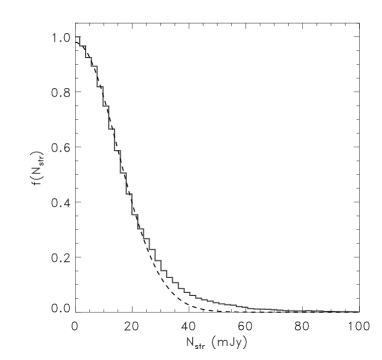
Figure 7: Distribution of the structure noise in the ELAIS N1 field. The solid line (histogram) represents the measured $N_{\mathrm{str}}$ values over the whole field. The dashed line represents the Gaussians fitted to the low amplitude regime (see text for details).

As seen in this figure the distribution of $N_{\mathrm{str}}$ is Gaussian-like, with an extended tail toward high structure noise values. In brighter cirrus regions the distribution of cirrus fluctuations can be well separated from the fluctuation of the CFIRB and the contribution of the instrument noise. In those fields the fluctuation distribution can be well described by a Gaussian one (Kiss et al. 2003). In the following we assume that this distribution can be applied for the fluctutions in the faint ELAIS fields as well. Fig. 7 can be used to estimate the source confusion limits of the ELAIS fields. We fitted a Gaussian to the lower noise regime ($N_{\mathrm{str}}$ $<$ 20 mJy) of the $N_{\mathrm{str}}$ distribution of the N1, N2, N3 and S1 fields, which resulted in a $\sigma$ of 14.8, 12.8, 13.4, and 17.1 mJy, respectively. With the point spread function fraction coefficient of $f_{\mathrm{psf}}$ = 0.61 for a C100 camera pixel at 90 $\mu$m the 3–$\sigma$ source confusion limit is $\sim$70 mJy. Moreover, it is worth to mention that the cosmic far-infrared background has an expected fluctuation power of $\sim$7 mJy at this wavelength for the C100 camera detector pixels (Kiss et al. 2001), which contributes to the final width of the $N_{str}$ distribution. Eliminating this value from the width of the Gaussians, the remaining contributions of the cirrus fluctuations and the instrument noise would be $\sim$60 mJy at 3–$\sigma$.

9 Source counts

9.1 ELAIS counts

Table 3: Integral number counts in the ELAIS survey. S is the flux in mJy; N is the number of sources per deg² with flux larger than S; The upper and lower uncertainties in the counts which come from Poisson error and the correction of the Eddington bias are indicated. N_s is the number of sources with flux larger than S.

S	N($>S$)	N_s
mJy	deg-2
95	17.02$\pm$4.50/4.30	185
177	7.93$\pm$1.19/1.83	90
330	2.70$\pm$0.74/0.74	30
614	0.77$\pm$0.39/0.39	9

Table 4: Normalized differential number counts. Columns are : flux range for each bin in mJy; the bin centre; dN/dS $\times$ S^2.5 are the number counts per bin normalized to the Euclidian law in deg^-2Jy^1.5 (the bin centre in linear scale was used for the normalisation); The upper and lower uncertainties in the counts which come from Poisson error and the correction of the Eddington bias are indicated. N_s is the number of sources per bin.

flux bin	bin centre	dN/dS $\times$ S2.5	N_s
mJy	mJy	deg-2 Jy1.5
95–176	135	0.74$\pm$0.20/0.22	95
176–329	253	1.11$\pm$0.24/0.24	60
329–613	471	1.04$\pm$0.27/0.27	21
613–1142	877	0.85$\pm$0.32/0.32	7

Integral and normalized differential source counts are given in Tables 3 and 4 for 185 sources brighter than 95mJy (above this flux, the uncompleteness and Eddington bias corrections are lower than 25 and 15% respectively). Uncertainties in the counts represent the contribution of Poisson errors and the Eddington bias correction. The possibility that some sources could be solar system bodies was rejected in Sec.3. Moreover as stated in Paper III, given that there are no bright 12-$\mu$m sources in the ELAIS fields (to avoid saturating ISOCAM) we do not expect any ’photospheric’ stars to be detected at 90 $\mu$m as these would have a 90 $\mu$m flux $\leq$ 10 mJy. Finally, the 3–$\sigma$ limit of the cirrus and instrumental noise was estimated in Sect. 8 to be $\sim$60 mJy. Therefore it is very likely that all the selected sources above 95 mJy are extragalactic.

Figure 8 shows ELAIS integral counts (filled circles) at 90 $\mu$m compared with results of Juvela et al. (2000; asterisks), the preliminary analysis of ELAIS (Paper I; open circles), Linden-Vørnle et al. (2000; squares), Matsuhara et al. (2000) from the Lockman Hole observations (triangle) and the new analysis of the Lockman Hole performed by Rodighiero et al. (2003) (diamonds). IRAS points (x symbols) are also shown for galaxies in the PSCz catalogue (Saunders et al. 2000) with a selection of galactic latitude ($|b|>20$) and low IRAS flags ($f_{\rm qual}<3$) at 100 $\mu$m and fluxes brighter than 2Jy as it becomes incomplete at fainter level (see Paper III for details). The dashed line is the no-evolution model from Franceschini et al. (2001). Correction factors of 1/1.06 and 1/0.76 derived from the comparison of the FCS calibration with standard stars model predictions (Sect. 6.1) and with IRAS (Sect. 6.2) are also shown.

Our results extend IRAS counts by more than one order of magnitude. They are in very good agreement with the preliminary analysis of ELAIS and confirm the departure from the Euclidian slope found in Paper I. Integral counts in the range 0.095-1Jy are well fitted with a straight line of the form:

$$\log_{10}(N)=(-1.68\pm 0.09)\times\log_{10}(S\mathrm{[Jy]})-(0.43\pm 0.07)$$ (4)

Figure 8: Integral source counts at 90 $\mu$m for ELAIS (filled circles). Error bars are Poisson error plus the uncertainties on the Eddington bias. Flux uncertainties are 7% resulting from the use of the FCS for calibration purposes (Sect. 2.3). Correction factors of 1/1.06 and 1/0.76 derived from the comparison of the FCS calibration with standard stars model predictions and with IRAS respectively are shown as -0.03 dex and +0.12 dex error bars at (-1.3,-2.0). Source counts from Juvela et al. (2000; asterisks), the preliminary analysis of ELAIS (Paper I; open circles), Linden-Vørnle et al. (2000; squares), Matsuhara et al. (2000; triangle) and Rodighiero et al. (2003; diamonds) are shown for comparison. IRAS counts (x symbols) are shown for galaxies in the PSCz catalogue. The dashed line is the no-evolution model from Franceschini et al. (2001).

9.2 Comparison with evolutionary models

Figure 9: Normalized differential source counts for ELAIS (filled circles) at 90 $\mu$m. Error bars include Poisson error and the uncertainties on the Eddington bias. Correction factors of 1/1.06 and 1/0.76 are shown as -0.03 dex and +0.12 dex error bars at (1.5,-1.0). Lockman Hole counts from Rodighiero et al. (2003) are also shown (diamonds). IRAS counts (crosses) are shown for galaxies in the PSCz catalogue. The solid line is the no-evolution model from Franceschini et al. (2001). The dashed and dotted line represent models A and E of Guiderdoni et al. (1998), respectively. The dash-dotted line are the counts predicted by Rowan-Robinson (2001) for his cosmological model with $\Omega_{0}=0.3$ and $\Lambda=0.7$.

Figure 10: Same as 9 but the dashed-dotted, dashed and dotted lines are the models of Pearson (2001), Franceschini et al. (2001) and Lagache, Dole & Puget (2003), respectively.

Recent observations in the FIR and sub-millimeter regimes have considerably improved evolutionary models in the past 5 years. In the following, we briefly describe the main characteristics of evolutionary models by Guiderdoni et al. (1998), Rowan-Robinson (2001), Pearson (2001), Franceschini et al. (2002), Lagache et al. (2003) and compare the predictions to differential number counts measured in the ELAIS survey on Figs. 9 and 10.

1. Guiderdoni et al. 1998 have designed a family of semi-analytic evolutionary scenarios within the context of hierarchical growth of structures according to the cold dark matter model, with prescriptions for dissipative and non-dissipative collapses, star formation and feedback. Differences between these scenarios only concern the efficiency of star formation on a dynamical time-scale, the IMF and the extinction. In Figure 9 we compare our results with two of their models:

   Scenario A contains a mix of two broad types of populations, one with a ’quiescent’ star formation rate, the other proceeding in bursts with a high evolution rate and fitting the SFR density at low z;

   Scenario E includes an additional population of heavily-extinguished galaxies (ULIGs) and is qualified as the best fit by Guiderdoni et al. as it nicely reproduces the Cosmic Optical Background and the Cosmic Infrared Background.

   If model A is systematically below the measured counts, the addition of a ULIGs population shifts the predictions upwards and the model E falls in excellent agreement with the observations as it was suggested in Paper III based on the brightest sources.

2. The models of Rowan-Robinson (2001) include four spectral components: infrared cirrus, an M82-like starburst, an Arp 220-like starburst, and an active galactic nucleus dust torus. The proportion of each spectral type are chosen for consistency with IRAS and SCUBA colour-luminosity relations and with the fraction of AGNs as a function of luminosity in 12 $\mu$m samples.

   The prediction of the Rowan-Robinson model for the cosmological model with $\Omega_{0}=0.3$ and $\Lambda=0.7$ is compared with the observed counts on Figure 9. The model is in good agreement with the observations down to fluxes of $\sim 200$ mJy within the error bars. At fainter fluxes it gives a slightly too high number of sources.

3. The model of Pearson and Rowan-Robinson (1996) consists of non-evolving spiral and elliptical components mixed with an evolving population of starburst galaxies, active galactic nuclei and a hyperluminous galaxy component. The model is in agreement with the source counts at 60 $\mu$m and the faint radio counts at 1.4 Ghz and provides a good estimate of the cosmic infrared background observed with COBE at 500 $\mu$m.

   More recently, Pearson (2001) used the framework of the Pearson and Rowan-Robinson galaxy evolution model and constrains the evolution in the galaxy population with the observed counts and background measurement derived from ISO and SCUBA observations. Pearson found that a strong evolution in both density and luminosity of the ULIG population can account for the source counts from 15 $\mu$m to the submillimetre region, as well as explain the peak in cosmic infrared background at $\sim$ 140 $\mu$m.

   The prediction for this model is also shown on Figure 10. The model provides a good fit to the ELAIS observations although it seems to become too high at fluxes fainter than $\sim$ 100 mJy compared to the Lockman Hole counts of Rodighiero et al. 2003.

4. The model of Franceschini et al. (2001) assumes that the extragalactic population is composed of three components with different evolution properties: (1) a non-evolving population of spirals; (2) a population of strongly evolving starburst galaxies and type-II AGNs; (3) a population of type-I AGNs which does not contribute significantly to the counts. This model was optimized to reproduce the mid-IR counts and redshift distribution. In particular, the two components of the fast evolving population were required to reproduce the shape of the $15\mu$m counts.

   The model of Franceschini is plotted on Figure 10 and gives a good estimate of the observed counts. The increase in number counts seen at fluxes fainter than $\sim 100$ mJy is probably the far-infrared counterpart of the upturn detected in the mid-infrared (Elbaz et al. 1999, Chary and Elbaz 2001, Mazzei et al. 2001; Serjeant et al. 2000). The ELAIS 90 $\mu$m data do not allow us to test if this predicted feature is real or not but Rodighiero et al. (2003) have shown it is compatible within the error bars with the faint counts in the “Lockman Hole”.

5. Lagache, Dole & Puget (2003) have developed a phenomenological model which fits all the existing counts and redshift distributions from the mid-infrared to the submillimetre range together with the intensity and fluctuation of the cosmic infrared background. Their model is based on the evolution of galaxy luminosity function with redshift for a population of starburts and normal galaxies.

   The model of Lagache, Dole & Puget 2003 (shown on Figure 10 is compatible with ELAIS counts (although slightly higher) around 1 Jy and with a larger discrepancy at fainter level ($S\leq 200$ mJy) where the model continues to increase while the observed counts decrease.

10 Summary and discussion

We have used a new method to reduce ISOPHOT measurements in the 4 main areas of the ELAIS survey at 90 $\mu$m. With a total area of more than 12 deg², the ELAIS survey represents the largest area covered in a single programme with ISO.

The relative uncertainty in flux coming from the FCS calibration estimated from the sky background level differences of all rasters is 7 per cent.

On the one hand, the comparison of measured fluxes with models for standard stars shows a strong correlation with a mean ratio of ISOPHOT to model values of $1.06\pm 0.02$. On the other hand, the comparison with the IRASFSC catalogue for IRAS sources detected in the survey gives a mean ratio of ISOPHOT to IRAS values equal to 0.76$\pm$0.17.

Simulations of artificial sources on the final maps spanning a wide range of flux were used to estimate flux and positional uncertainties, completeness and the Eddington bias corrections. The completeness of the survey is about $80\%$ at 100 mJy.

We present a source list of 237 reliable sources with fluxes larger than 70 mJy, signal-to-noise $\geq 3$ for the 4 large ELAIS fields. The full version of the catalogue is available at http://www.blackwell-synergy.com.

Sources detected at 90 and 170 $\mu$m in the FIRBACK survey (Dole et al. 2001) have an average colour temperature of $T_{C}=19K$ with all sources lying in the range 13-25K in agreement with Stickel et al. (2001) in the ISO Serendipity Survey (Stickel et al. 1998).

The ELAIS counts extend the IRAS counts by more than one order of magnitude in flux and show significant departure from the no-evolution model as detected in other ISO surveys from the mid- to the far-infrared.

There is in general a good agreement between ELAIS and other 90 $\mu$m source counts and in particular with the deeper counts measured in the Lockman Hole (Rodighiero et al. 2003). Differential number counts measured in the ELAIS regions at 90 $\mu$m are compared to recent evolutionary models. Among few models which were compared to our counts, the model of Franceschini et al. (2001) and the scenario E of Guiderdoni et al. (1998) give the best agreement with the observations.

However, the latter model is a factor of $\sim 2.5$ below the counts measured at 170 $\mu$m in two of the ELAIS regions (Dole et al. 2001) related to the present paper. On the other hand Matsuhara et al. (2000) found that the scenario E model prediction of Guiderdoni et al. is in close agreement with the 170 $\mu$m number counts in the small area of the “Lockman Hole” (see also Kawara et al. 1998) but their 90 $\mu$m integral counts are significantly above the model.

The nature and redshift distributions of the ELAIS galaxies can test the various models and their hypothesis e.g. distinguishing the different galaxy populations on which these models are built. This will also help to clarify the origin of the differences seen in the number counts of the various ISO surveys at different wavelengths.

The 90 $\mu$m luminosity function is presented in Serjeant et al. (2004) and Rowan-Robinson et al. (2004) present results based on the ELAIS final-band merged catalogue combining the ISO and ground-based observations in the ELAIS fields.

11 Acknowledgments

We thank the referee Yasunori Sato for detailed comments and suggestions which helped us improve the manuscript. It is a pleasure to acknowledge Peter Ábrahám and Ulrich Klaas for very useful discussions about ISOPHOT calibration and data analysis. We also thank Guilaine Lagache and Michael Linden-Vørnle for making their results available to us in electronic version. We are grateful to Emmanuel Bertin for valuable advice on the use of SExtractor.

Ph. Héraudeau acknowledges support from the EU TMR Network “SISCO” (HPRN-CT-2002-00316).

C. del Burgo acknowledges support from the EU TMR Network “POE” (HPRN-CT-2000-001380).

ELAIS was supported by EU TMR Network FMRX-CT96-0068 and PPARC grant GR/K98728.

This paper is based on observations with ISO  an ESA project with instruments funded by ESA member states (especially the PI countries: France, Germany, the Netherlands and the United Kingdom) and with participation of ISAS and NASA. The ISOPHOT data were processed using PIA, a joint development by the ESA Astrophysics Division and the ISOPHOT consortium led by MPI für Astronomie, Heidelberg. Contributing Institutes are DIAS, RAL, AIP, MPIK, and MPIA.

The development and operation of ISOPHOT were supported by MPIA and funds from Deutsches Zentrum für Luft- und Raumfarht (DLR, formerly DARA). The ISOPHOT Data Center at MPIA is supported by Deutsches Zentrum für Luft- und Raumfarht e.V. (DLR) with funds of Bundesministerium für Bildung und Forschung, grant No. 50 QI 9801 3.

References

- Barger (1998) Barger, A. J., Cowie, L. L., Sanders, D. B., Fulton, E., Taniguchi, Y., Sato, Y., Kawara, K., Okuda, H., 1998, Nature, 394, 248
- Bertin96 (1996) Bertin E., Arnouts S., 1996, A&AS, 117, 393
- Bertin97 (1997) Bertin E., Dennefeld M., Moshir M., 1997 A&A, 323, 685
- Cohen (1999) Cohen M., Walker R.G., Carter B., Hammersley P., Kidger M., Noguchi K., 1999, AJ, 117, 1864.
- Chary (2001) Chary R., Elbaz D., 2001, ApJ, 556, 562
- Devriendt (2000) Devriendt J.E.G., Guiderdoni B., 2000, A&A, 363, 851
- del Burgo2003a (2003a) del Burgo C., Héraudeau Ph., Ábrahám P., 2003a, in C. Gry, S. Peschke, J. Matagne, P. Garcia-Lario, R. Lorente, & A. Salama.,ed., Proc. “Exploiting the ISO Data Archive”, ESA SP-511, European Space Agency,339
- del Burgo2003b (2003b) del Burgo C., Ábrahám P., Klaas U., Héraudeau Ph.,2003b, in L. Metcalfe, A. Salama, S.B. Peschke and M.F. Kessler, ed., Proc. “The calibration legacy of the ISO Mission”, ESA SP-481, European Space Agency, 351
- Dole (2001) Dole H.,et al., A&A, 372, 364
- Dunne (2001) Dunne L., Eales S. A. 2001, MNRAS, 327, 697
- Eales (2000) Eales S., Lilly S., Webb T., Dunne L., Gear W., Clements D., Yun M., 2000, AJ, 120, 2244
- Eddington (1913) Eddington A.S., 1913, MNRAS, 73, 359
- Efstathiou (2000) Efstathiou A.,et al., 2000, MNRAS, 319, 1169 (Paper III)
- Elbaz (1999) Elbaz D.,et al., 1999, A&A, 351, L37
- Franceschini (2001) Franceschini A., Aussel H., Cesarsky C.J., Elbaz D., Fadda D., 2001, A&A, 378, 1
- Fruchter02 (2002) Fruchter A.S., Hook R.N., 2002, PASP, 114, 144
- Fruchter97 (1997) Fruchter A.S., Hook R. N., in Proc. Applications of Digital Image Processing XX, ed. Tescher A.G., 1997, SPIE Vol. 3164, 120
- Gabriel (1997) Gabriel C., Acosta-Pulido J., Heinrichsen I., Morris H., Tai W.-M., 1997, in Hunt H., Payne H.E., eds., A.S.P. Conf. Ser. Vol. 125, Astronomical Data Analysis Software and Systems VI, p. 108
- Gruppioni (2002) Gruppioni C., Lari C., Pozzi F., Zamorani G., Franceschini A., Oliver S., Rowan-Robinson M., Serjeant S., 2002, MNRAS, 335, 831
- Guiderdoni (1998) Guiderdoni B., Hivon E., Bouchet F.R., Maffei B., 1998, MNRAS, 295, 877
- Hacking (1987) Hacking P., Houck J.R., 1987, ApJS, 63, 311
- Hacking (1991) Hacking P. B., Soifer B.T., 1991, ApJ, 367, 49
- Hacking (1987) Hacking P., Condon J.J., Houck J.R., 1987, ApJ, 316, L15
- Hammersley (1998) Hammersley P., Jourdain de Muizon M., Kessler M.F., Bouchet P., Joseph R.D., Habing J., Salama A., Metcalfe L., 1998, AAS, 128, 207.
- Hauser (2001) Hauser M. G., Dwek E., 2001, ARA&A, 39, 249
- Herbstmeier (1998) Herbstmeier U. et al. 1998, A&A, 332, 739
- Hughes98 (1998) Hughes D., Dunlop, J., 1998, in Observational Cosmology with the New Radio Surveys, Proceedings of a Workshop held in Puerto de la Cruz, Tenerife, Canary Islands, Spain, 13-15 January 1997, Dordrecht: Kluwer Academic Publishers, 1998, Astrophysics and space science library (ASSL) Series vol no: 226, p.259
- Juvela (2000) Juvela M., Mattila K. and Lemke D., 2000, A&A, 360, 813
- Kalluri (1998) Kalluri S., Arce G.R., 1998, ’Adaptive weighted myriad filter algorithms for robust signal processing in alpha-stable noise environments’, IEEE Transaction on signal Processing, 46, 322 (or at http://www.ee.udel.edu/signals/pubs/nonlinear/kalluri_tsp97.ps)
- Kawara (1998) Kawara, K. et al., 1998, A&A, 336, L9
- Kessler96 (1996) Kessler M. F. et al. 1996, A&A, 315, 27
- Kessler00 (2000) Kessler M. F. 2000, in Infrared space astronomy, today and tomorrow. Les Houches, Session LXX, held 3-28 August, 1998. École de Physique des Houches - UJF & INPG - Grenoble, a NATO Advanced Study Institute. Edited by F. Casoli, J. Lequeux, and F. David. Published in cooperation with the NATO Scientific Affair Division by Springer-Verlag, Berlin, Paris, 2000, p.29
- Kiss01 (2001) Kiss Cs., Ábrahám P., Klaas U., Juvela M., Lemke D., 2001, A&A 379, 1611
- Kiss03 (2003) Kiss Cs., Ábrahám P., Klaas U., Lemke D., Héraudeau Ph., del Burgo C., Herbstmeier U., 2003, A&A, 399, 177
- Lagache (2003) Lagache G., Dole H., Puget J.-L., 2003, MNRAS, 338, 555
- Laureijs99 (1999) Laureijs R. J. 1999, Point spread function fractions related to the ISOPHOT C100 and C200 arrays, http://www.iso.vilspa.esa.es/users/expl_lib/PHT_list.html
- Laureijs01 (2003) Laureijs R. J., Klaas U., Richards P. J., Schulz B. & Ábráham P., 2003, in L. Metcalfe, A. Salama, S.B. Peschke and M.F. Kessler, ed., The ISO Handbook Vol. IV, PHT - The Imaging Photo-Polarimeter, ESA-SP/1262, European Space Agency
- Lemke (1996) Lemke D. et al., 1996, A&A, 315, 64
- Lonsdale (2003) Lonsdale C. J. et al., 2003, PASP, 115, 897
- Linden (2000) Linden-Vørnle et al., 2000, A&A, 359, 51
- Matsuhara (2000) Matsuhara H. et al., 2000 A&A 361, 407
- Mazzei (2001) Mazzei P., Aussel H., Xu C., Salvo M., De Zotti G., Franceschini A., 2001, NewA, 6, 265
- Moshir (1992) Moshir M., Kopman G., Conrow T. A. O., IRAS Faint Source Survey, Explanatory supplement version 2, 1992, JPL D-10015 8/92 (Pasadena: JPL)
- Muller02a (2002) Müller T.G., Hotzel S., Stickel M., 2002, A&A, 389, 665
- Muller02b (2002) Müller T.G., Lagerros J.S.V. 2002, A&A, 381, 324
- Muller98 (1998) Müller T.G., Lagerros J.S.V. 1998, A&A, 338, 340
- Murdoch (1973) Murdoch H.S., Crawford D.F., Jauncey D.L., 1973, ApJ, 183, 1
- Oliver (1995) Oliver S. et al., 1995, in Proc. 35th Herstmonceux Conf. Wide Field Spectroscopy and the Distant Universe, eds. S.J. Maddox, A. Aragon-Salamanca, World scientific, 274
- Oliver (2000) Oliver S. et al., 2000, MNRAS, 316, 749, (Paper I)
- Oliver (2002) Oliver S. et al., 2002, MNRAS, 332, 536
- Oliver (1992) Oliver S., Rowan-Robinson M., Saunders W., 1992, MNRAS, 256, 150
- Pearson (1996) Pearson C. P., Rowan-Robinson M., 1996, MNRAS, 283, 174.
- Pearson (2001) Pearson C. P., 2001, MNRAS, 325, 1511
- Pearson (2004) Pearson C. P., 2004, MNRAS, 347, 1113
- Puget (1999) Puget J. L. et al., 1999, A&A, 345, 29
- Rodighiero (2003) Rodighiero, G., Lari, C., Franceschini, A., Gregnanin, A., Fadda, D., 2003 MNRAS, 343, 1155
- RowanRobinson (2001) Rowan-Robinson M., 2001, ApJ, 549, 745
- RowanRobinson (2004) Rowan-Robinson M. et al., 2004, MNRAS, in press
- Saunders (2000) Saunders W., et al., 2000, MNRAS, 317, 55
- Scott (2002) Scott S. E. et al., 2002, MNRAS, 331, 817
- Serjeant (2000) Serjeant S. et al., 2000, MNRAS, 316, 768
- Serjeant (2004) Serjeant S. et al., 2004, MNRAS, in Press
- Sodroski (1994) Sodroski T. J. et al., 1994, ApJ, 428, 638
- Stickel (1998) Stickel M. et al., 1998, A&A, 336, 116
- Stickel (2000) Stickel M. et al., 2000, A&A, 359, 865
- Stickel (2001) Stickel M. et al., 2001, in Pilbratt G.L., Cernicharo J., Heras A.M., Prusti T., Harris R., eds., ESA-SP Vol. 460, The Promise of the Herschel Space Observatory, p. 109
- Stickel (2003) Stickel M., Bregman J. N., Fabian A. C., White D. A., Elmegreen D. M., 2003, A&A, 397, 503
- Takeuchi (2001) Takeuchi T., et al., 2001, PASJ, 53, 37
- Teerikorpi (1998) Teerikorpi P., 1998, A&A 339, 647
- Tody (1993) Tody D. 1993, in Hanisch R.J., Brissenden R.J.V., Barnes J., eds., ASP Conf. Ser. Vol. 52, Astronomical Data Analysis Software and Systems II, p. 173
- Webb (2003) Webb T. M., et al., 2003, ApJ, 587, 41
- Wang (2002) Wang Y. P., 2002, A&A 383, 755
- Xu (2003) Xu C. K., Lonsdale C. J., Shupe D. L., Franceschini A., Martin, C., Schiminovich D., 2003 ApJ, 587, 90