Cosmic-ray propagation properties for an origin in SNRs

Abstract

We have studied the impact of cosmic-ray acceleration in SNR on the spectra of cosmic-ray nuclei in the Galaxy using a series expansion of the propagation equation, which allows us to use analytical solutions for part of the problem and an efficient numerical treatment of the remaining equations and thus accurately describes the cosmic-ray propagation on small scales around their sources in three spatial dimensions and time. We found strong variations of the cosmic-ray nuclei flux by typically 20% with occasional spikes of much higher amplitude, but only minor changes in the spectral distribution. The locally measured spectra of primary cosmic rays fit well into the obtained range of possible spectra. We further showed that the spectra of the secondary element Boron show almost no variations, so that the above findings also imply significant fluctuations of the Boron-to-Carbon ratio. Therefore the commonly used method of determining CR propagation parameters by fitting secondary-to-primary ratios appears flawed on account of the variations that these ratios would show throughout the Galaxy.

1 Introduction

The origin of cosmic-rays (CR) is one of the major problems in modern astrophysics. In that quest two possible strategies may be followed:

• one may search for high-energy emission from the source regions themselves, for the CR density must be very high therein. Particle acceleration at supernova remnant (SNR) shock waves is regarded as the most probable mechanism for providing Galactic cosmic rays at energies below $10^{15}$ eV on account of the power requirements (Blandford & Eichler, 1987). The recent detections of non-thermal X-ray synchrotron radiation from the four supernova remnants SN1006 (Koyama et al., 1995), RX J1713.7-3946 (Koyama et al., 1997; Slane et al., 1999), Cas A (Allen et al., 1997; Gotthelf et al., 2001), and RCW86 (Bamba, Koyama, and Tomida, 2000; Borokowski et al., 2001; Rho et al., 2002) support the hypothesis that at least CR electrons are accelerated predominantly in SNR. The evidence for CR nucleon acceleration in SNR is at best controversial (Berezhko, Ksenofontov, and Völk, 2002; Reimer & Pohl, 2002).

• one may also construct models for the diffusive propagation of CRs in the Galaxy and compare their predictions with observed CR spectra at earth (e.g. Strong & Moskalenko, 1998; Maurin et al., 2001; Taillet & Maurin, 2003). The relation between primary CRs, which have been accelerated somewhere in the Galaxy, and secondary CRs, which are produced in interactions of CRs with ambient gas, then allows to determine the propagation parameters such as the diffusion coefficient, the size of the diffusion region, and others. Nearly all published studies of that kind assume steady-state conditions.

Already in 1969, Lingenfelter (1969) found the CR energy density at earth to vary due to nearby SN, given the CR are accelerated at these sites. A few years ago Pohl & Esposito (1998) showed for CR electrons that in case of SN origin the CR electron spectrum would vary in space and time throughout the Galaxy. The purpose of this paper is to present a time-dependent propagation model for CR nucleons. In particular we aim to address the following questions:

• would a SNR origin of CR nucleons also lead to significant fluctuations of the CR density in the Galaxy, which then would modify secondary-to-primary ratios from their steady-state values? If that was the case, we would have to re-think the way we infer CR propagation parameters from their locally observed spectra.

• are there any signatures in the CR distribution in the Galaxy, that might permit to infer a SNR origin of CR nucleons on the grounds of locally observed CR spectra and the diffuse Galactic gamma-ray emission?

For that purpose we have developed a method to numerically solve the propagation equation based on a series expansion, which allows us to use analytical solutions for part of the problem and an efficient numerical treatment of the remaining equations. As described in detail in section 2 this technique allows us to accurately follow the CR propagation on small scales around their sources in three spatial dimensions and time. In section 3 we discuss the results of these calculations with respect to the CR density distribution and in section 4 with respect to CR spectra, respectively.

2 The Model

2.1 The basic equations

Our investigations are performed in the framework of a diffusion model of CR propagation, so we use a continuity equation for the differential CR number density, $N$:

$$\frac{\partial N}{\partial t}-S=\nabla\left(k\nabla N\right)-\Omega v\sigma N.$$ (1)

with particle speed $v$ and total spallation cross section $\sigma$. We consider the diffusion zone to be a disk of radius $R=20$ kpc (cf. Webber et al., 1992) and height $2H$ (see Fig. 1), where $H$ is determined below. The density of the interstellar gas is assumed to decrease with distance from the galactic plane, $z$, with a profile

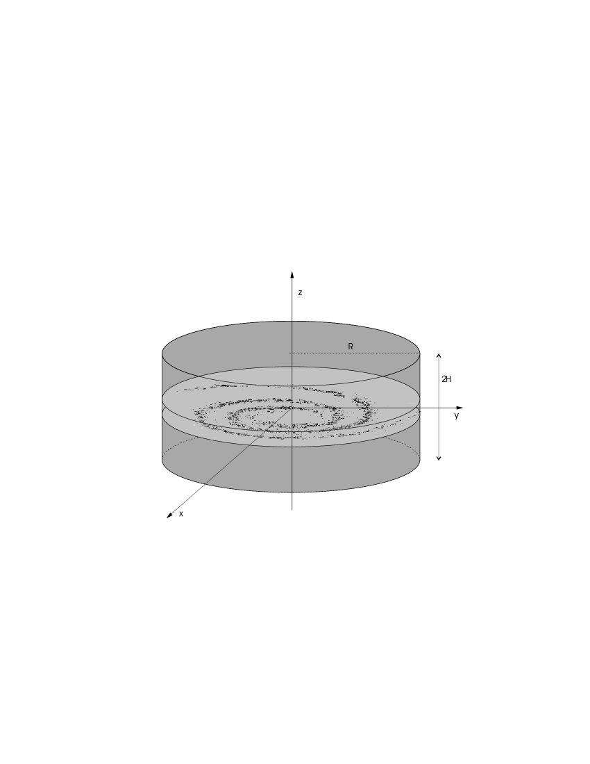
Figure 1: Sketch of the geometry used in our calculations. We assume that the Galactic disk with radius $R$ is filled with interstellar gas and the CR sources. The density of the interstellar gas decreases quasi-exponentially in the halo. The height of the entire diffusion zone is $2H$.

$$\Omega(z) = \frac{n_{0}}{{\rm cosh}\left(z\,h_{g}\right)}\,.$$ (2)

The parameters $n_{0}$ = 1.24 cm^-3 and $h_{g}$ = 30 kpc^-1 corresponding to a column density of $\sim 6.2\cdot 10^{20}\,$cm^-2 are chosen to be consistent with the calculations by, e.g., Webber et al. (1992) or Berezinskiĭ (1990). The chemical composition of the ISM, which consists mainly of hydrogen and some heavier elements, is taken into account by multiplying the gas density Eq. (2) by a factor of 1.3, as it is done by Mannheim & Schlickeiser (1994) for the calculation of CR-induced pion production in the ISM.

The diffusion coefficient, $k$, depends on the particle rigidity $\zeta$ = $p/q$ with particle momentum $p$ and charge $q$. The form

$$k = \left\{{k_{0}\left(\frac{\zeta}{\zeta_{0}}\right)^{0.6}\,\,\,\,\,\qquad{\rm for\,\,}\zeta\geq\zeta_{0}\atop k_{0}\left(\frac{\zeta}{\zeta_{0}}\right)^{-0.48}\qquad{\rm for\,\,}\zeta<\zeta_{0}}\right.$$ (3)

with $\zeta_{0}=4$ GV/c is chosen to reproduce the observed Boron-to-Carbon ratio.

As we consider discrete, point-like sources, the source term $S$ in Eq. (1), is in fact the sum of the contributions of many source, each of which has the same temporal and spectral form. For the time dependence we assume a linear growth with an exponential cut-off, with the source spectra being power laws with index $s$ in particle rigidity $\zeta$.

$$q_{j}\left(\zeta,t\right)=\hat{q}_{j}\cdot\left(t-t_{j}\right){\rm exp}\left(-\frac{t-t_{j}}{20\,{\rm kyr}}\right)\Theta\left(t-t_{j}\right)\cdot\left(\frac{\zeta}{\zeta_{0}}\right)^{-s}.$$ (4)

We assume the SN explosions to be stochastic events. Their effect on the CR spectra can thus be studied by the method of Monte-Carlo simulations, so many possible CR spectra are calculated using randomly chosen sets of CR sources. We used the rejection method (Press et al., 1993) to compute the quantities $r_{j},\varphi_{j},z_{j}$ for the location, $t_{j}$ for the ignition time, and $\hat{q}_{j}$ for the source strength. The position of the CR sources in azimuth, $\varphi_{j}$, is uniformly distributed, whereas for the radial distribution we use the form suggested by Case & Bhattacharya (1996), and for the vertical distribution we use the same profile as for the density of interstellar gas. Then

$$\tilde{P}_{S}(r,z)=\frac{1}{{\rm cosh}(z\,h_{g})}\left(\frac{b\,r}{a\,r_{s}}\right)^{a}\cdot{\rm exp}\left(\frac{a\,r_{s}-b\,r}{r_{s}}\right).$$ (5)

with parameters $a=1.69$, $b=3.33$, $r_{s}=8.5$ as taken from the paper of Case & Bhattacharya (1996).

The ignition time, $t_{j}$, and the source strength, $\hat{q}_{j}$, are uniformly distributed on the intervals $[t_{\rm start};t_{\rm end}]$ and $[0;1]$, respectively. We have also performed simulations using a detailed model of the spatial and temporal evolution of the nearby star-forming region Gould’s belt (Perrot & Grenier, 2003).

This leaves $k_{0}$, the halo height $H$ and the source spectral index $s$ as free parameters, which we determined by fitting the Boron-to-Carbon ratio and the survival fraction of ¹⁰Be calculated for the steady-state case to measured data. Solar modulation is taken into account using the force field approximation (Gleeson & Axford, 1968) with modulation parameter $\Phi\,=\,500\,$MV. In the steady-state case the best-fit parameters are $k_{0}=0.26\,$kpc²Myr^-1, $H$ = 2 kpc, and $s$ = 2.1, as shown in Fig. 2.

Figure 2: Best fits of Boron-to-Carbon data (upper panel) and ¹⁰Be/⁹Be data (lower panel), compared to data by Engelmann et al. (1990) ($\triangle$), Dwyer & Meyer (1987) ($\Diamond$), Krombel & Wiedenbeck (1988) ($\Box$), and Orth et al. (1978) ($\times$) for the Boron-to-Carbon ratio and from Connell (1998), Garcia-Munoz et al. (1981), Hams et al. (2001), Lukasiak et al. (1994), de Nolfo et al. (2001), and Wiedenbeck & Greiner (1980) for the ¹⁰Be to ⁹Be ratio, respectively.

2.2 The method of computation

To determine the influence of the discrete nature of SNR as CR sources on the CR distribution and spectra, one has to solve the CR propagation equation Eq. (1) with high resolution, both in space and time. With today’s computers, however, it is not possible to calculate the CR density with a spatial resolution sufficient to investigate point-like sources in an adequate way. One should note that the grid size in finite-difference algorithms, e.g. those in the widely used code Galprop (Strong & Moskalenko, 2001), in principle has to be much finer than the size of the presumed sources, for one has to deal with large gradients in the CR flux on small scales. Thus, the accuracy of representation of the CR density on a fixed grid is highly questionable. One way out of this quandary may be the implementation of adaptive mesh-refinement techniques in the finite-difference algorithms. The way we followed is to use an analytical ansatz that breaks down the problem of solving the propagation equation Eq. (1) into many small tasks, that are easily solved on pc-style hardware. The series ansatz to solve Eq. (1) will be in detail described in the next section. We also developed a method to spread the task of solving the propagation equation onto many computers, so the spatial resolution obtained is only limited by the number of computers available.

2.3 The Ansatz

Considering the cylindrical geometry of our Galaxy (with radius $R$ and height $2H$, see Fig. 1), we assume the gas distribution $\Omega$ and diffusion coefficient $k$ to be independent of $r$ and $\varphi$. Then the CR transport equation Eq. (1) can be written in cylindrical coordinates:

$$\frac{\partial N}{\partial t}-S = k(p)\left\{\frac{1}{r}\frac{\partial N}{\partial r}+\frac{\partial^{2}N}{\partial r^{2}}+\frac{1}{r^{2}}\frac{\partial^{2}N}{\partial\varphi^{2}}+\frac{\partial^{2}N}{\partial z^{2}}\right\}-\Omega(z)v\sigma N.$$ (6)

We start by expanding the desired solution $N$ in a Fourier series in $\varphi$ and a Fourier-Bessel series in $r$:

$$N = \frac{1}{\pi}\sum_{n}\sum_{m}\left(A_{nm}\cdot\cos\left(n\varphi\right)+B_{nm}\cdot\sin\left(n\varphi\right)\right)\frac{\jmath_{n}\left(\alpha_{nm}r\right)}{\left(\jmath_{n}^{\prime}\left(\alpha_{nm}R\right)\right)^{2}}$$ (7)

with $\alpha_{nm}$ being the $m$th solution of $\jmath_{n}\left(\alpha_{nm}R\right)=0$ (in ascending order). We also expand the individual source terms for the point-like sources

$$S = \sum_{i}q_{i}(p,t)\delta\left(\vec{r}-\vec{r}_{i}\right),$$ (8)

where $q_{i}(p,t)$ is the time and momentum dependence of the particular source and $\vec{r}_{i}$ its position, into the same series in $r$ , $\varphi$

$$S = \sum_{i}q_{i}(p,t)\delta\left(z-z_{i}\right)$$

$$\times\sum_{n}\sum_{m}\left(\cos\left(n\varphi\right)\cos\left(n\varphi_{i}\right)+\sin\left(n\varphi\right)\sin\left(n\varphi_{i}\right)\right)\frac{\jmath_{n}\left(\alpha_{nm}r\right)\jmath_{n}\left(\alpha_{nm}r_{i}\right)}{\left(\jmath_{n}^{\prime}\left(\alpha_{nm}R\right)\right)^{2}}.$$

For extended and continuous sources, e.g. for secondary CRs, one has to use the Fourier-Bessel representation of the source distribution of the particle in question.

Inserting Eq. (7) and Eq. (2.3) into Eq. (6) and using the orthonormality of sine and cosine and the analogous property of the Bessel functions (Watson, 1944)

$$\int_{0}^{R}\frac{\jmath_{n}\left(\alpha_{nm}r\right)\jmath_{n}\left(\alpha_{\ n\mu}r\right)}{\left(\jmath_{n}^{\prime}\left(\alpha_{nm}R\right)\right)^{2}}rdr = \delta\left(m,\mu\right)$$ (10)

one obtains equations for the expansion coefficients $A_{nm}$

$$\frac{\partial A_{nm}}{\partial t}-S_{nm}^{A} = k(p)\left\{-\alpha_{nm}^{2}A_{nm}+\frac{\partial^{2}A_{nm}}{\partial z^{2}}\right\}-\Omega(z)v\sigma A_{nm}$$ (11)

with

$$S_{nm}^{A} = \sum_{i}q_{i}(p,t)\cos\left(n\,\varphi_{i}\right)\frac{\jmath_{n}\left(\alpha_{nm}r_{i}\right)}{\left(\jmath_{n}^{\prime}\left(\alpha_{nm}a\right)\right)^{2}}$$ (12)

and similar equations for $B_{nm}$

$$\frac{\partial B_{nm}}{\partial t}-S_{nm}^{B} = k(p)\left\{-\alpha_{nm}^{2}B_{nm}+\frac{\partial^{2}B_{nm}}{\partial z^{2}}\right\}-\Omega(z)v\sigma B_{nm}$$ (13)

with

$$S_{nm}^{B} = \sum_{i}q_{i}(p,t)\sin\left(n\,\varphi_{i}\right)\frac{\jmath_{n}\left(\alpha_{nm}r_{i}\right)}{\left(\jmath_{n}^{\prime}\left(\alpha_{nm}a\right)\right)^{2}}.$$ (14)

These equations are not analytically solvable for arbitrary $\Omega(z)$, therefore one has to use numerical methods. The advantage of this ansatz is, that it is possible to solve these one-dimensional PDEs simultaneously on many computers. Also, the resolution at a given point obtained in $r,\varphi$ merely depends on the number of coefficients in the series ansatz, Eq. (7), that is actually computed.

As the $\alpha_{nm}$’s increase monotonically with $n$ and also with $m$, one sees from Eq. (11), that for large $m,n$ we have $k(p)\alpha^{2}\gg\Omega(z)v\sigma B_{nm}$ and therefore, the latter term may be neglected. In this case an analytical solution is known.

2.4 CR distribution due to a single source

Before we start solving Eq. (11) and Eq. (13), we have to determine the number of coefficients to be taken into account in the ansatz Eq. (7). Evidently, the spatial resolution in $r,\,\varphi$ direction of the solution obtained by the ansatz Eq. (7) depends on the number of coefficients used and also on the distance $r$ from the origin. As we are mainly interested in the CR density in the vicinity of the Sun, we determine the number of coefficients by comparing the solutions of the propagation equation Eq. (6) obtained by a truncated series according to ansatz Eq. (7) with the solution of the propagation equation for a spherical source with a radius of $\rho_{s}\,=\,50$ pc, located at the position of the Sun. To ease the calculations we neglect the geometry of the Galaxy, assuming the loss processes not to depend on the spatial coordinates. This is permitted if we consider only the vicinity of the source for a limited time after the SN explosion. So, we study the source in an uniformly distributed ISM.

First, we derive a solution for a spherical source. In this case, placing the source at the origin of our coordinate system provides us with spherical symmetry, i.e. the solution only depends on the radial coordinate, $\rho$. We further restrict ourselves to one fixed particle momentum $p$. Then Eq. (1) can be written as

$$\frac{\partial N}{\partial t}-S=k\left(\frac{\partial^{2}N}{\partial\rho^{2}}+\frac{2}{\rho}\frac{\partial N}{\partial\rho}\right)-bN$$ (15)

with $b=\Omega\,v\,\sigma$. The source $S$ has the temporal form given in Eq. (4), so we have

$$S = \hat{q}_{i}\cdot\left(t-t_{i}\right){\rm exp}\left(-\frac{t-t_{i}}{\tau}\right)\Theta\left(t-t_{i}\right)\Theta\left(\rho_{s}-\rho\right).$$ (16)

Without loss of generality, we set $\hat{q}_{i}\,=\,1$ and $t_{i}\,=\,0$.

For Eq. (15) one can find the Green’s function

$$G = \frac{1}{8\pi\sqrt{\pi}\sqrt{k}}\frac{1}{\rho\,\rho_{0}\sqrt{t-t_{0}}}{\rm exp}\left(-b\left(t-t_{0}\right)\right)$$ (17)

$$\times{\rm exp}\left(-\frac{\rho^{2}+\rho_{0}^{2}}{4\,k\left(t-t_{0}\right)}\right){\rm sinh}\left(\frac{2\,\rho\,\,\rho_{0}}{4k\left(t-t_{0}\right)}\right).$$

For a verification that Eq. (17) is indeed a Green’s function for Eq. (15) and a short discussion on how to obtain it, we refer to Appendix A.

Thus, we obtain the solution of Eq. (15) with sources Eq. (16) by the convolution

$$N\left(\rho,t\right) = \int_{\rho_{0}=0}^{\rho_{s}}\int_{t_{0}=0}^{t}G\left(\rho,\rho_{0},t,t_{0}\right)\cdot S\left(\rho_{0},t_{0}\right)\,d\rho_{0}dt_{0}$$ (19)

$$= \int_{\rho_{0}=0}^{\rho_{s}}\int_{t_{0}=0}^{t}\frac{1}{8\pi\sqrt{\pi}\sqrt{k}}\frac{1}{\rho\,\rho_{0}\sqrt{t-t_{0}}}{\rm exp}\left(-b\left(t-t_{0}\right)\right){\rm exp}\left(-\frac{\rho^{2}+\rho_{0}^{2}}{4\,k\left(t-t_{0}\right)}\right)$$

$$\times{\rm sinh}\left(\frac{\rho\,\,\rho_{0}}{2\,k\left(t-t_{0}\right)}\right)\cdot\,t_{0}{\rm exp}\left(-\frac{t_{0}}{\tau}\right)$$

$$\times\Theta\left(t_{0}\right)\Theta\left(\rho_{s}-\rho\right)\rho_{0}^{2}d\rho_{0}dt_{0}.$$

The $\rho_{0}$ integration can be performed analytically, which leads to

$$N\left(\rho,t\right) = \int_{t_{0}=0}^{t}\left\{-2\,\sqrt{k\left(t-{t_{0}}\right)}{\,\,\exp\left({{\frac{-{\rho_{s}}^{2}-{\rho}^{2}}{4\,k\,\left(t-{t_{0}}\right)}}}\right)}\,\sinh\left({\frac{\rho_{s}\rho}{2\,k\left(t-{t_{0}}\right)}}\right){\rho}^{-1}\right.$$ (20)

$$\left.+\frac{\sqrt{\pi}}{2}\left({\rm erf}\left(\frac{1}{2}\,{\frac{\rho_{s}-\rho}{\sqrt{k\left(t-{t_{0}}\right)}}}\right)+{\rm erf}\left(\frac{1}{2}\,{\frac{\rho_{s}+\rho}{\sqrt{k\left(t-{t_{0}}\right)}}}\right)\right)\right\}$$

$$\times{\exp\left({b\left({t_{0}}-t\right)}\right)}{t_{0}}\,{\exp\left(-\frac{t_{0}}{\tau}\right)}dt_{0}.$$

Unfortunately, this integral is not solvable analytically. It was computed numerically using a Riemann sum. The result is plotted in Fig. 3, where we also plotted the solution of Eq. (1), using addends with $m\leq 210$ and $n\leq 311$ in ansatz Eq. (7), which turned out to be the best tradeoff of numerical complexity versus spatial accuracy. This solution using ansatz Eq. (7) describes well, both in $r-$ and $\varphi$-direction, the spatial evolution of the CR density around a spherical source.

Figure 3: Comparison of CR density due to a spherical source with radius 50 pc given by Eq. (20) (solid line) and that computed using Eq. (7) with 312 coefficients used for the series in $n$ and 210 coefficients used in the series in $m$; cuts in $r$ (dotted line) and $\varphi$ (dashed line) direction, for different times from source “ignition”.

3 Signatures of Discrete Sources in the Galactic Cosmic Ray Distribution

In this section we represent first results of our investigation as to what extent the SN origin of CR affects the density distribution of Galactic CR. We study the temporal evolution and the fluctuations in the CR density, using the methods developed in the previous section.

3.1 Randomly Distributed Sources

We now consider the time-dependent propagation equation Eq. (6) that we solve using the ansatz Eq. (7) for several source distributions. As a first step we performed a calculation for CR point sources that are randomly distributed in the Galactic plane. For that purpose we chose ¹⁶O, for it is regarded as the most abundant primary CR element beyond helium. For this calculation and those described in the following sections, the CR density $N$ was computed using ansatz Eq. (7). The corresponding coefficients $A_{nm}$, $B_{nm}$ were obtained numerically using a semi-implicit scheme based on the Du Fort-Frankel (Du Fort & Frankel, 1953) and leapfrog schemes. We started the calculation of the temporal evolution of the CR density ,$N$, from the appropriate steady state solutions, which were calculated using the package TOMS638 (Houstis et al., 1985a, b).

For the source function we use $n_{q}$ randomly distributed point sources with a radial probability distribution given by Eq. (5). Considering only one CR primary element at a time, we have for the source term $S$ in Eq. (6):

$$S(r,\varphi,z,t) = \sum_{i=1}^{n_{q}}q_{i}\left(t,p\right)\delta\left({\vec{r}}-{\vec{r}_{i}}\right)$$ (21)

with the source strengths $q_{i}$ defined in Eq. (4), and $\vec{r}_{i}$ the locations of the $i$th source. The number of sources, $n_{q}\,=\,150000$, was chosen to reproduce the local supernova surface density of 25 SN per Myr and kpc² of the Galactic disk (Grenier, 2000). We calculated CR densities for several random SN distributions in the Galactic disk, each for a time interval of $10\,$Myr.

Figure 4: Temporal variation of the ¹⁶O CR primary density at the position of the Sun, for 10 GeV per nucleon (upper panel) and 5 TeV per nucleon (lower panel).

Figure 5: The density of ¹⁶O at $E=10\,$GeV per nucleon in a 400 pc $\times$ 400 pc section of the Galactic plane ($z=0$) during a local SN event for several times (in Myr). The Sun ($r=8.5\,$kpc, $\phi=1.025$) is positioned at the center. The local CR density is strongly influenced by nearby SN, although the excess quickly disappears.

In these calculations, the coefficients with $1\leq m\leq 210$ and $0\leq n\leq 311$ of the series ansatz Eq. (2.3) were computed. This yields a resolution in $r$, $\varphi$ of $\sim$ 170 pc at the position of the Sun. The grid spacing in $z$ is 20 pc, the time step is 1 kyr.

Computing the series Eq. (2.3) at the position of the Sun gives the time variation of the CR density at this position, as is shown in Fig. 4, where the CR density for an energy of 10 GeV per nucleon (upper panel) and for an energy of 5 TeV per nucleon (lower panel) is plotted versus time. These figures illustrate that the density of CR with an energy of 5 TeV shows more rapid fluctuations than at an energy of 10 GeV on account of the energy dependence of the diffusion coefficient.

The variations in the CR density at a given location, shown in Fig. 4, have a typical amplitude of about 20 per cent with occasional spikes reaching 100 per cent. The latter mainly occur due to nearby SN explosions, as illustrated in Fig. 5, where the temporal evolution of the CR density at an energy of 10 GeV per nucleon is shown for a 400 pc$\,\times\,$400 pc section of the Galactic plane. Variations of the same order of magnitude of the local CR energy density due to nearby SN have been found by Lingenfelter (1969) when he investigated the contribution of these SN to the CR energy density near our Sun, using a simple diffusion type model only considering losses due to escape. The perturbation in the CR density due to the source stays almost localized and does not spread out.

3.2 The influence of Gould’s Belt Star-Burst Region

The local distribution of stars and the ISM is dominated by the so-called Gould’s Belt (Pöppel, 1997). Of particular interest for our investigations is the enhanced SN rate within the belt (Grenier, 2000). The kinematics of the belt can be modeled by an expanding ring of gas, assuming an initial explosive event (Perrot & Grenier, 2003). Its age is estimated to be about 30 Myr which implies that with regard to our calculations, which cover the last 10 Myr, not only its presence, but also the still evolving geometry of the belt has to be taken into account. We assume that the enhanced supernova rate applies to the entire volume of Gould’s belt, i.e. we neglect a possible delay on account of the main-sequence phase of very massive stars. The probability distribution for supernova explosion would then be given by the time-dependent expansion model of Perrot & Grenier (2003) in addition to the stationary large-scale SN distribution in the Galaxy (see Eq.5).

The results displayed in Fig. 6 show an enhanced variation of the local CR density due to the locally increased SN rate compared to the case without Gould’s Belt, that has been given in the last section and is shown in Fig. 4. The locally enhanced SN rate also leads to a locally increased mean CR density which is most pronounced at low energies or, in other words, SNR need less efficiency as CR accelerators to replenish the galactic cosmic rays.

Figure 6: Same as Fig. 4, assuming a locally enhanced SN rate in Gould’s Belt.

3.3 Secondary Cosmic Ray Particles

In section 3.1 we showed that the density of CR primary nuclei may vary up to about one order of magnitude in space and time. To investigate to what extent this is also true for secondary CR nuclei and, therefore, whether there are any effects on the ratio of secondary to primary CR isotopes, we further performed calculations including secondary nuclei. As the ratio of Boron to Carbon is widely used to quantify the parameters of various propagation models, we considered the isotopes ¹²C, which was assumed to be pure primary and ¹¹B which was assumed to be produced solely by interactions of the primary ¹²C with the interstellar matter. The results of these calculations are shown

Figure 7: Temporal variation of the CR primary density ¹²C (upper panel) and secondary ¹¹B (lower panel) at the position of the Sun at energy of 10 GeV per nucleon. The deviation from the average value for the CR secondary density is way smaller than that for the CR primary density.

in Fig. 7, where we plot, as in Fig. 4, the CR density at 10 GeV per nucleon versus time for the primary isotope ¹²C (upper panel) and the secondary isotope ¹¹B (lower panel), both at the position of the Sun. Fig. 7 shows that, although the density of the primary CR varies by a factor of 2, as expected from the previous calculations, the variation of the secondary CR particles is only a few per cent. This statement holds true also for higher particle energies.

Figure 8: The density of primary CRs (upper panel) and that of secondary CRs (lower panel) plotted as a function of distance from the Galactic plane at $R_{0}=8.5$ kpc from the Galactic center. The left column is for a particle energy of 10 GeV per nucleon, and the right column applies to particles at 5 TeV energy. We show the density distributions at four arbitrarily chosen instances of time, indicated by different line-styles.

Having analyzed the variations of the CR density with time (Fig. 4, Fig. 7) and in the Galactic plane (Fig. 5), we now are interested in the variations of the CR flux perpendicular to the Galactic disk. In Fig. 8, we compare the densities of primary (upper panels) and secondary (lower panels) CR perpendicular to the Galactic plane, for CR energies of 10 GeV (left panels) and 5 TeV (right panels), respectively, at four different instances of time, indicated by different line-styles.

As in the case of Fig. 7, where we plotted the density of CR primary and secondary particles at one position in the Galactic plane versus time, these figures show, that there is only a marginal variation of the CR secondary distribution perpendicular to the Galactic plane, despite rather large variations in the CR primary distributions. This behavior depends only weakly on the particle energy. Nevertheless, for particle energies of 5 TeV, there is a variation in the density of CR secondaries at $z=0$ of roughly 10%. These findings have far-reaching consequences for the ratio of secondary to primary CR, as discussed in the next section.

4 Global signatures of an SNR origin of cosmic rays

Equipped with a technique to calculate the spatial and temporal distribution of CR primary and secondary elements with SN-like objects as sources, we now discuss the observational implications for CR astrophysics. We discuss the calculated spectra themselves and also compare them with measurements for the CR primary elements ¹⁶O and ¹²C.

To obtain a measure of the variations of the CR spectra at the position of the Sun, we simulated 240 possible CR spectra both for the standard Galactic plane distribution of supernovae as given by Eq.5 and for the Gould’s belt supernovae in addition to that.

In Fig. 9 and Fig. 11 (upper panel), we give the range of possible spectra at the position of the Sun for the primary nuclei ¹⁶O and ¹²C, respectively, for the case of randomly distributed sources (upper panels) and including also Gould’s Belt (lower panels). In the same figures we compare the range of calculated spectra with data by Engelmann et al. (1990) ($\times$), Müller et al. (1991) ($\Box$), Orth et al. (1978) ($\Diamond$) and Simon et al. (1980) ($\triangle$). Those authors provide data for Carbon as well as oxygen. We model the effect of solar modulation using the force field approximation (Gleeson & Axford, 1968), assuming a modulation parameter of $\Phi\,=\,500$ MV. These locally measured data fit quite well in our calculated range of possible spectra.

The amplitude of variations in the possible primary CR nuclei spectra is clearly seen and does not increase much with energy as is the case, e.g., for the electrons (section 4.3). The level of computational noise is very much less than the calculated fluctuation amplitudes for the primary CRs, as is indicated by the small level of fluctuations calculated for the secondary CRs in section 4.2. The local clustering of sources (section 4.1) due to Gould’s Belt enhances the fluctuation amplitude, so the model fits the measurements even better. We also note a slight steepening of the averaged spectrum.

Fig. 10 shows some examples of our calculated ¹²C spectra. Note that the spectra mostly vary in their amplitudes, and only weakly in their forms. We now discuss these findings in detail.

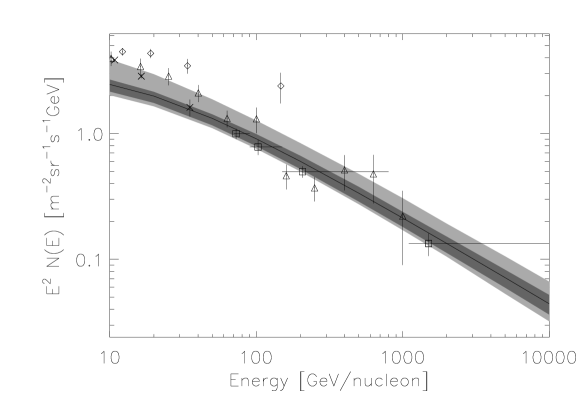
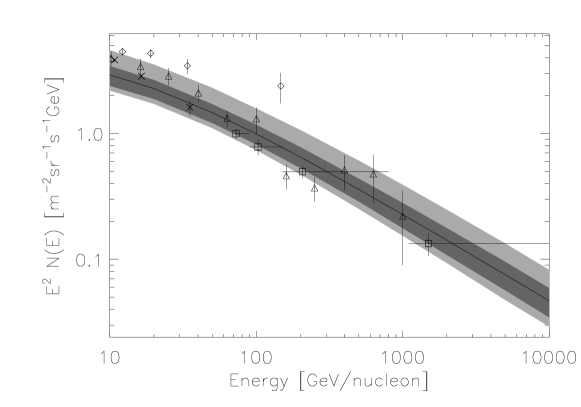
Figure 9: The range of possible ${}^{16}{\rm O}$ spectra with (lower panel) and without (upper panel) Gould’s Belt compared with measurements taken with balloons or satellites. The dark grey band shows the 68% containment probability range at each given energy and the light grey band gives the 95% range. The solid line marks the averaged (steady-state) spectrum. All spectra are as at the top of the atmosphere.

Figure 10: Sample of possible ¹²C spectra, given at the top of the atmosphere.

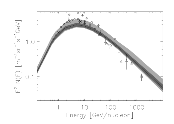
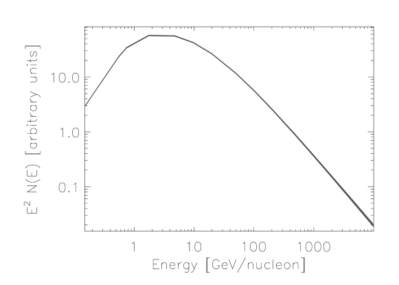
Figure 11: Same as Fig. 9 but for ${}^{12}{\rm C}$ (upper panel) and ${}^{11}{\rm B}$, which is assumed to be purely secondary, produced from primary ¹²C only (lower panel).

4.1 Effects due to the Clustering of Sources

We investigated the effects of a local clustering of sources using Gould’s Belt as an example. Our results are shown in Fig. 9 for the CR primary nucleus ¹⁶O and in Fig. 11 for CR secondary nucleus ¹¹B in each case with and without considering Gould’s Belt. Local clustering of discrete CR sources leads to an enhanced fluctuation margin in the CR primary spectra and on average to a slightly steeper spectrum. The slight steepening of the spectrum is caused by the energy dependence of diffusion: the high-energy particles fill a somewhat larger volume than do their low-energy siblings. Then the differential number density must be softer than the total number spectrum, except for the short time interval the low-energy particle need to diffusively propagate to the location at which the spectrum is measured. Almost no effects of Gould’s Belt can be seen in the CR secondary spectra.

4.2 Implications on the Secondary to Primary Ratio

Comparing the range of possible spectra for primary CR (see Fig. 9) and secondary CR (see Fig. 11) reveals that the variation in the possible CR nuclei spectra is much higher for primary nuclei than for secondary nuclei. Thus, the variation in the primary spectra should also be visible in the secondary-to-primary ratios. As the variation in the amplitude of the CR primary spectra is stronger than that of the spectral form, one should expect the secondary-to-primary ratios to vary mostly in amplitude but not so much in the spectral form. Taillet & Maurin (2003) show using a steady-state scenario that the CR measured at the earth only probe the CR propagation parameters in a rather small domain, and thus outside this domain the CR fluxes and the secondary-to-primary ratios may be different. Our calculations reveal that even if the propagation parameters do not vary, there is a variation in the secondary-to-primary ratio due to discrete sources. So provided CR nuclei are accelerated at SNR or other kinds of discrete sources, one must account for fluctuations in the ratio of secondary to primary CR particles, e.g. the Boron-to-Carbon ratio, which is widely used to determine the parameters of CR propagation models. In particular, the ratio should decrease in the vicinity of a source. Thus it is important to know whether or not we live in the vicinity of a recent supernova, as has been proposed by some authors (see Erlykin & Wolfendale (1997) and subsequent papers).

4.3 Comparison With Cosmic Ray Electrons

We now compare our results derived for CR nuclei with the findings of Pohl & Esposito (1998) for CR electrons. Evidently, the fluctuation amplitude in the CR electron spectra strongly grows with energy, whereas that of CR nuclei spectra hardly depends on the particle energy (see e.g. Fig. 11). Kinks and dents are possible in CR electron spectra but are virtually not seen in the spectra of CR nuclei as shown in Fig.10.

5 Summary and discussion

We have studied the impact of CR acceleration in SNR on the spectra of CR nuclei in the Galaxy. We found strong evidence that this assumption leads to CR spectra, which show significant variations in space and time. The behavior of the CR nuclei resembles that of protons, as suggested by first computations (Strong & Moskalenko, 2001), but differs considerably from that of CR electrons (Pohl & Esposito, 1998).

We have developed a method to numerically solve the propagation equation based on a series expansion, which allows us to use analytical solutions for part of the problem and an efficient distributed computing for the remainder. This method was employed to calculate the CR densities in the Galactic disk with high spatial ($\Delta z\,=\,20\,$pc) and temporal ($\Delta t\,=\,1\,$kyr) resolution for the primary nuclei ¹⁶O, ¹²C and the secondary nucleus ¹¹B for various distributions of SNR. This method allowed for the first time to calculate the CR densities in the Galactic disk with the high spatial and temporal resolution required to follow the CR density fluctuations caused by an SNR origin. We also studied the impact of a locally enhanced SN rate within Gould’s Belt, a nearby star-forming region.

We found strong variations of the CR nuclei flux by typically 20% with occasional spikes of much higher amplitude, but only minor changes in the spectral distribution. The locally measured primary CR spectra fit well into the obtained range of possible spectra. We further showed that the spectra of the secondary element Boron show almost no variations, so that the above findings also imply significant fluctuations of the Boron-to-Carbon ratio. Therefore the commonly used method of determining CR propagation parameters by fitting secondary-to-primary ratios appears flawed on account of the variations that these ratios would show throughout the Galaxy.

Some indications that the CR flux varies in the Galaxy are given by the observation of the diffuse $\gamma$-ray emission in our Galaxy. Digel et al. (2001) performed $\gamma$-ray observations of the outer Galaxy. Their analysis of the diffuse $\gamma$-ray emission from giant molecular clouds in the Monoceros region suggests that the CR flux in the local Galactic arm and the neighboring Perseus arm differ, i.e. the data suggests an enhancement of the CR density in the Perseus arm. These observations would be well explained by the variations in the flux of CR nuclei that results from a SNR origin.

Hunter et al. (1997) find that the spectrum of the diffuse $\gamma$-ray emission toward the inner Galaxy can not be explained by the assumption that the locally observed CR spectrum and electron-to-proton ratio hold throughout the Galaxy. At $\gamma$-ray energies above some GeV, where the spectrum is presumably dominated by CR-nucleon-induced radiation, they find that the $\gamma$-ray flux measured exceeds by about 50% that expected if the local CR spectrum and electron-to-proton ratio hold throughout the Galaxy. These findings are difficult to explain by the calculations presented above as being caused by spectral variations of the CR nuclei flux, for we find these to be rather small. We have, however, neglected the possibility of a dispersion in the source spectral indices, which has been proposed as an explanation of the GeV excess (cf. Büsching et al., 2001).

6 Acknowledgements

IB acknowledges support by the Bundesministerium fr̈ Bildung und Forschung through DLR grant 50 OR 0006 and by the Deutsche Forschungsgemeinschaft through Sonderforschungsbereich 591. MP acknowledges support by NASA under award No. NAG5-13559.

Appendix A Green’s Function for the Spherical Symmetric Propagation Equation

In case of spherical symmetry, the propagation equation in spherical coordinates reads (Eq. (15)):

$$\frac{\partial N}{\partial t}-S=k\left(\frac{\partial^{2}N}{\partial r^{2}}+\frac{2}{r}\frac{\partial N}{\partial r}\right)-bN.$$ (A1)

Using the ansatz

$$N = {\rm exp}\left(-\frac{1}{T}t\right)\cdot\phi$$ (A2)

leads to an equation for $\phi=\phi(r,\varphi,t)$

$$\frac{\partial\phi}{\partial t}-{\rm exp}\left(\frac{1}{T}t\right)\cdot S=k\left(\frac{\partial^{2}\phi}{\partial r^{2}}+\frac{2}{r}\frac{\partial\phi}{\partial r}\right).$$ (A3)

For this equation, a Green’s function can be found in the literature (Butkovskiy, 1982). It reads

$$\bar{G} = \Theta\left(t-t_{0}\right)\frac{1}{4\pi\sqrt{\pi}\sqrt{k}}\frac{1}{r\,r_{0}\sqrt{t-t_{0}}}$$ (A4)

$$\times{\rm exp}\left(-\frac{r^{2}+r_{0}^{2}}{4\,k\left(t-t_{0}\right)}\right){\rm sinh}\left(\frac{2\,r\,r_{0}}{4k\left(t-t_{0}\right)}\right).$$

Re-substituting Eq. (A2), we finally get

$$G = \Theta\left(t-t_{0}\right)\frac{1}{4\pi\sqrt{\pi}\sqrt{k}}\frac{1}{r\,r_{0}\sqrt{t-t_{0}}}\exp\left(-b\left(t-t_{0}\right)\right)$$ (A5)

$$\times{\rm exp}\left(-\frac{r^{2}+r_{0}^{2}}{4\,k\left(t-t_{0}\right)}\right){\rm sinh}\left(\frac{2\,r\,r_{0}}{4k\left(t-t_{0}\right)}\right)$$

which we now show to be indeed the desired fundamental solution of Eq. (A1). For the derivatives we have:

$$\frac{\partial G}{\partial r} = -\frac{1}{r}\,G-\frac{r}{2k\left(t-t_{0}\right)}\,G+\frac{r_{0}}{2k\left(t-t_{0}\right)}\frac{{\rm cosh}\left(\frac{2\,r\,r_{0}}{4k\left(t-t_{0}\right)}\right)}{{\rm sinh}\left(\frac{2\,r\,r_{0}}{4k\left(t-t_{0}\right)}\right)}\,G$$ (A6)

$$\frac{\partial^{2}G}{\partial r^{2}} = \frac{2}{r^{2}}\,G+\frac{1}{2k\left(t-t_{0}\right)}\,G-\frac{r_{0}}{k\,r\left(t-t_{0}\right)}\frac{{\rm cosh}\left(\frac{2\,r\,r_{0}}{4k\left(t-t_{0}\right)}\right)}{{\rm sinh}\left(\frac{2\,r\,r_{0}}{4k\left(t-t_{0}\right)}\right)}\,G+\left(\frac{r}{2k\left(t-t_{0}\right)}\right)^{2}G$$ (A7)

$$-2\left(\frac{1}{2k\left(t-t_{0}\right)}\right)^{2}r\,r_{0}\frac{{\rm cosh}\left(\frac{2\,r\,\,r_{0}}{4k\left(t-t_{0}\right)}\right)}{{\rm sinh}\left(\frac{2\,r\,r_{0}}{4k\left(t-t_{0}\right)}\right)}G+\left(\frac{r_{0}}{2k\left(t-t_{0}\right)}\right)^{2}G$$

$$\frac{\partial G}{\partial t} = -\frac{1}{2\left(t-t_{0}\right)}\,G-b\,G+\frac{r^{2}+r_{0}^{2}}{4k\left(t-t_{0}\right)^{2}}\,G-\frac{2\,r\,r_{0}}{4k\left(t-t_{0}\right)^{2}}\frac{{\rm cosh}\left(\frac{2\,r\,\,r_{0}}{4k\left(t-t_{0}\right)}\right)}{{\rm sinh}\left(\frac{2\,r\,\,r_{0}}{4k\left(t-t_{0}\right)}\right)}\,G$$ (A8)

$$+\delta\left(t-t_{0}\right)\frac{1}{\Theta\left(t-t_{0}\right)}.$$

Inserting the above into the Eq. (A1) yields

$$\left\{\frac{-1}{2\left(t-t_{0}\right)}-b+\frac{r^{2}+r_{0}^{2}}{4k\left(t-t_{0}\right)^{2}}-\frac{2\,r\,r_{0}}{4k\left(t-t_{0}\right)^{2}}\frac{{\rm cosh}\left(\frac{2\,r\,\,r_{0}}{4k\left(t-t_{0}\right)}\right)}{{\rm sinh}\left(\frac{2\,r\,\,r_{0}}{4k\left(t-t_{0}\right)}\right)}+\frac{\delta\left(t-t_{0}\right)}{\Theta\left(t-t_{0}\right)}\right\}G$$ (A9)

$$= k\Biggl{\{}\frac{2}{r^{2}}\,G+\frac{1}{2k\left(t-t_{0}\right)}\,G-\frac{r_{0}}{k\,r\left(t-t_{0}\right)}\frac{{\rm cosh}\left(\frac{2\,r\,r_{0}}{4k\left(t-t_{0}\right)}\right)}{{\rm sinh}\left(\frac{2\,r\,r_{0}}{4k\left(t-t_{0}\right)}\right)}\,G+\left(\frac{r}{2k\left(t-t_{0}\right)}\right)^{2}G$$

$$-2\left(\frac{1}{2k\left(t-t_{0}\right)}\right)^{2}r\,r_{0}\frac{{\rm cosh}\left(\frac{2\,r\,\,r_{0}}{4k\left(t-t_{0}\right)}\right)}{{\rm sinh}\left(\frac{2\,r\,r_{0}}{4k\left(t-t_{0}\right)}\right)}G+\left(\frac{r_{0}}{2k\left(t-t_{0}\right)}\right)^{2}G$$

$$+\frac{2}{r^{2}}\,G-\frac{1}{k\left(t-t_{0}\right)}\,G+\frac{r_{0}}{r\,k\left(t-t_{0}\right)}\frac{{\rm cosh}\left(\frac{2\,r\,r_{0}}{4k\left(t-t_{0}\right)}\right)}{{\rm sinh}\left(\frac{2\,r\,r_{0}}{4k\left(t-t_{0}\right)}\right)}\,G\Biggr{\}}-b\,G+S.$$

Comparing terms, we get

$$\left\{\frac{-1}{2\left(t-t_{0}\right)}+\frac{r^{2}+r_{0}^{2}}{4k\left(t-t_{0}\right)^{2}}{{\rm sinh}\left(\frac{2\,r\,\,r_{0}}{4k\left(t-t_{0}\right)}\right)}+\frac{\delta\left(t-t_{0}\right)}{\Theta\left(t-t_{0}\right)}\right\}G-S$$ (A10)

$$= k\Biggl{\{}+\frac{1}{2k\left(t-t_{0}\right)}\,G{{\rm sinh}\left(\frac{2\,r\,r_{0}}{4k\left(t-t_{0}\right)}\right)}\,G+\left(\frac{r}{2k\left(t-t_{0}\right)}\right)^{2}G{{\rm sinh}\left(\frac{2\,r\,r_{0}}{4k\left(t-t_{0}\right)}\right)}G+\left(\frac{r_{0}}{2k\left(t-t_{0}\right)}\right)^{2}G$$

$$+\frac{2}{r^{2}}\,G-\frac{1}{k\left(t-t_{0}\right)}\,G{{\rm sinh}\left(\frac{2\,r\,r_{0}}{4k\left(t-t_{0}\right)}\right)}\,G\Biggr{\}}.$$

So finally we have

$$S = \frac{\delta\left(t-t_{0}\right)}{\Theta\left(t-t_{0}\right)}G.$$ (A11)

Here $S$ is the delta function for spherical polar coordinates, so we have to verify that the r.h.s. of Eq. (A11) is a representation of the delta function

$$S = \frac{1}{r^{2}}\delta\left(r-r_{0}\right)\delta\left(t-t_{0}\right).$$ (A12)

So with Eq. (A5), replacing the $\sinh$ by its definition, we have:

$$S = \delta\left(t-t_{0}\right)\frac{1}{8\pi\sqrt{\pi}\sqrt{k}}\frac{1}{r\,r_{0}\sqrt{t-t_{0}}}\exp\left(-b\left(t-t_{0}\right)\right)$$

$$\times\left(\exp\left(-\frac{\left(r-r_{0}\right)^{2}}{4\,k\left(t-t_{0}\right)}\right)-\exp\left(-\frac{\left(r+r_{0}\right)^{2}}{4\,k\left(t-t_{0}\right)}\right)\right).$$

Performing the limit for $t\to t_{0}$ on the r.h.s. leads to

$$\lim_{t\to t_{0}}\frac{1}{8\pi\sqrt{\pi}\sqrt{k}}\frac{1}{r\,r_{0}\sqrt{t-t_{0}}}\exp\left(-b\left(t-t_{0}\right)\right)$$

$$\times\left(\exp\left(-\frac{\left(r-r_{0}\right)^{2}}{4\,k\left(t-t_{0}\right)}\right)-\exp\left(-\frac{\left(r+r_{0}\right)^{2}}{4\,k\left(t-t_{0}\right)}\right)\right)$$

$$= \frac{1}{8\pi\sqrt{\pi}\sqrt{k}}\frac{1}{r\,r_{0}}\left(\lim_{t\to t_{0}}\frac{\exp\left(-\frac{\left(r-r_{0}\right)^{2}}{4\,k\left(t-t_{0}\right)}\right)}{\sqrt{t-t_{0}}}-\lim_{t\to t_{0}}\frac{\exp\left(-\frac{\left(r+r_{0}\right)^{2}}{4\,k\left(t-t_{0}\right)}\right)}{\sqrt{t-t_{0}}}\right)$$

$$= \left\{{0\,\,\,\,\,\,\,\,\quad{\rm for\,\,}r\not=r_{0}\atop\infty\,\,\,\,\,\quad{\rm for\,\,}r=r_{0}}\right.,$$ (A15)

as required for a delta function. To check the normalization of Eq. (A), we have to integrate over the spatial domain

$$I = \int_{r=0}^{\infty}\int_{\varphi=0}^{2\pi}\int_{\theta=0}^{\pi}Gr^{2}\sin\theta drd\varphi d\theta\Bigg{|}_{t=t_{0}}$$ (A16)

$$I = 4\pi\int_{r=0}^{\infty}Gr^{2}dr\Bigg{|}_{t=t_{0}}$$ (A17)

$$I = \lim_{t_{0}\to t}\int_{0}^{\infty}\Biggl{\{}\frac{r}{8\pi\sqrt{\pi}\sqrt{k}}\frac{1}{r_{0}\sqrt{t-t_{0}}}$$ (A18)

$$\times{\rm exp}\left(-\frac{r^{2}+r_{0}^{2}}{4\,k\left(t-t_{0}\right)}\right){\rm sinh}\left(\frac{2\,r\,r_{0}}{4k\left(t-t_{0}\right)}\right)dr\Biggr{\}}\Bigg{|}_{t=t_{0}}$$

With the integral 3.562.3 of Gradstein & Ryshik (1981)

$$\int_{0}^{\infty}r\,\exp\left(-\beta\,r\right)\sinh\left(\gamma\,r\right)dr = \frac{\gamma}{4\beta}\sqrt{\frac{\pi}{\beta}}\exp\left(\frac{\gamma^{2}}{4\beta}\right)$$ (A19)

we finally arrive at

$$I = \lim_{t_{0}\to t}\Biggl{\{}\frac{1}{2\sqrt{\pi}\sqrt{k}}\frac{1}{r_{0}\sqrt{t-t_{0}}}{\rm exp}\left(-\frac{r_{0}^{2}}{4\,k\left(t-t_{0}\right)}\right)\frac{r_{0}}{2}\sqrt{\pi\,4\,k\left(t-t_{0}\right)}$$ (A20)

$$\times{\rm exp}\left(\frac{r_{0}^{2}}{4\,k\left(t-t_{0}\right)}\right)\Biggr{\}}$$

$$I = 1$$ (A21)

which shows that the normalization is correct.

References

- Abramowitz & Stegun (1972) Abramowitz, M., & Stegun, I. A. 1972, Handbook of Mathematical Functions, Washington, National Bureau of Standards
- Allen et al. (1997) Allen, G. E., et al., 1997, ApJ, 487, L97
- Bamba, Koyama, and Tomida (2000) Bamba, A., Koyama, K., and Tomida, H., 2000, PASJ, 52, 1157
- Baring et al. (1999) Baring, M. G., Ellison, D. C., Reynolds, S. J., Grenier, I. A., Goret, P. 1999, ApJ, 513, 311
- Berezhko, Ksenofontov, and Völk (2002) Berezhko, E.G, Ksenofontov, L.T., and Völk, H.J., 2002, A&A, 395, 943
- Berezinskiĭ (1990) Berezinskiĭ V. S., Bulanov, S. V., Dogiel, V. A., Ginzburg, V. L., & Ptuskin, V. S. 1990, Astrophysics of cosmic rays, Amsterdam, North-Holland Elsevier Science Publishers B.V.
- Blandford & Eichler (1987) Blandford, R. D., & Eichler, D. 1987, Phys. Rep., 154, 1
- Borokowski et al. (2001) Borkowski, K. J., Rho, J., Reynolds, S. P., & Dyer, K. K. 2001, ApJ, 550, 334
- Büsching et al. (2001) Büsching I., Pohl M., Schlickeiser R. 2001, A&A, 377, 1056
- Butkovskiy (1982) Butkovskiy, A. G. 1982, Green’s Functions and Transfer Functions Handbook, Chichester, Ellis Horwood Ltd.
- Case & Bhattacharya (1996) Case, G., & Bhattacharya, D. 1996, A&AS, 120, 437
- Clark & Caswell (1976) Clark, D. H., & Caswell, J. L. 1976, MNRAS174, 267
- Connell (1998) Connell, J. J. 1998, ApJ, 501, L59
- de Nolfo et al. (2001) de Nolfo, G. A., et al. 2001 in Proc. 27th Int. Cosmic Ray Conf. (Hamburg), 1659
- Digel et al. (2001) Digel, S. W., Grenier, I. A., Hunter, S. D., Dame T. M., &Thaddeus P. 2001, ApJ, 555, 12
- Du Fort & Frankel (1953) Du Fort, E. C., & Frankel, S. P. 1953, Math. Tables and other Aids to Comp., 7, 135
- Dwyer & Meyer (1987) Dwyer, R., & Meyer, P. 1987, ApJ, 322, 981
- Engelmann et al. (1990) Engelmann, J. J., Ferrando, P., Soutoul, A., Goret, P., & Juliusson, E. 1990, A&A, 233, 96
- Erlykin & Wolfendale (1997) Erlykin, A.D., & Wolfendale, A.W. 1997, APh, 7, 1
- Garcia-Munoz et al. (1981) Garcia-Munoz, M., Simpson, J. A., Wefel, J. P. 1981 Proc. 17th Int. Cosmic Ray Conf. (Paris), 2, 72
- Gleeson & Axford (1968) Gleeson, L. J., & Axford, W. I. 1968, ApJ, 154, 1011
- Gotthelf et al. (2001) Gotthelf, E.V., Koralesky, B., Rudnick, L., Jones, T.W., Hwang, U., and Petre, R., 2001, ApJ, 552, 39
- Gradstein & Ryshik (1981) Gradstein, I., & Ryshik, I. 1981 Summen- Produkt- und Integraltafeln, Frankfurt am Main, Verlag Harri Deutsch
- Grenier (2000) Grenier I. A. 2000, A&A, 364, L93
- Hams et al. (2001) Hams, T., et al. 2001, Proc. 27th Int. Cosmic Ray Conf. (Hamburg), 1655
- Houstis et al. (1985a) Houstis, E. N., Mitchell, W. F., Rice, J. R. 1985, ACM TOMS 11, 379
- Houstis et al. (1985b) Houstis, E. N., Mitchell, W. F., & Rice, J. R. 1985, ACM TOMS 11, 416
- Hunter et al. (1997) Hunter S. D., et al. 1997, ApJ, 481, 205
- Koyama et al. (1995) Koyama, K., Petre, R., Gotthelf, E. V., Hwang, U., Matsuura, M., Ozaki, M., & Holt, S. S. 1995, Nature, 378, 255
- Koyama et al. (1997) Koyama, K., et al. 1997, PASJ, 49, L7
- Krombel & Wiedenbeck (1988) Krombel, K. E., & Wiedenbeck, M. E. 1988, ApJ, 328, 940
- LeBohec et al. (2000) LeBohec, S., et al. 2000, ApJ, 539, 209
- Letaw et al. (1983) Letaw, J.R., Silberberg, R., & Tsao, C.H.1983, ApJS, 51, 271
- Lingenfelter (1969) Lingenfelter, R. E., 1969, Nature, 224, 1182
- Lukasiak et al. (1994) Lukasiak, A., Ferrando, P., McDonald, F. B., & Webber, W. R. 1994, ApJ, 423, 426L
- Mannheim & Schlickeiser (1994) Mannheim, K., & Schlickeiser, R. 1994, A&A, 286, 983
- Maurin et al. (2001) Maurin, D., Donato, F., Taillet, R., Salati, P. 2001, ApJ, 555, 585
- Milne (1979) Milne, D. K. 1979, Austr. J. Phys. 32, 83
- Müller et al. (1991) Müller, D., Swordy, S. P., Meyer, P., L’Heureux, J., & Grunsfeld, J. 1991, ApJ, 374, 356
- Orth et al. (1978) Orth, C. D., Buffington, A., Smoot, G. F., & Mast, T. S. 1978, ApJ, 226, 1147
- Perrot & Grenier (2003) Perrot, C, & Grenier, I. A. 2003, A&A, 404, 519
- Pöppel (1997) Pöppel, W. 1997, Fundam. Cosmic Phys., 18, 1, (1997)
- Pohl & Esposito (1998) Pohl, M., & Esposito, J. 1998, ApJ, 507, 327
- Pohl et al. (2003) Pohl, M., Perrot, C., Grenier, I. A., & Digel, S. 2003, A&A, 409, 581
- Press et al. (1993) Press, W. H., Flannery, B. P., Teukolsky, S. A., & Vetterling, W. T. 1993, Numerical Recipes in C, Cambridge, University Press
- Reimer & Pohl (2002) Reimer, O., & Pohl, M. 2002, A&A, 390, 43
- Rho et al. (2002) Rho, J., Dyer, K.K., Borkowski, K.J., and Reynolds, S.P., 2002, ApJ, 581, 1116
- Schlickeiser (2002) Schlickeiser, R. 2002, Cosmic Ray Astrophysics, Berlin, Springer-Verlag
- Simon et al. (1980) Simon, M., Spiegelhauer, H., Schmidt, W. K. H., Siohan, F., Ormes, J. F., Balasubrahmanyan, V. K., & Arens, J. F. 1980, ApJ, 239, 712
- Slane et al. (1999) Slane, P., et al. 1999, ApJ, 525, 357
- Strong & Moskalenko (2001) Strong, A. W., & Moskalenko, I. V. 2001, Proc. 27th Int. Cosmic Ray Conf. (Hamburg), 1942
- Strong & Moskalenko (1998) Strong, A. W., & Moskalenko, I. V. 1998, ApJ, 509, 212
- Taillet & Maurin (2003) Taillet, R.,& Maurin 2003, A&A, 402, 971
- Watson (1944) Watson, G. N. 1944, A Treatise on the Theory of Bessel Functions, Cambridge, University Press
- Webber et al. (1992) Webber, W. R., Lee, M. A., & Gupta, M. 1992, ApJ, 390, 96
- Webber et al. (1990) Webber, W. R., Kish, J. C., & Schrier, D.A. 1990, Phys. Rev. C, 41, 566
- Wiedenbeck & Greiner (1980) Wiedenbeck, M. E., & Greiner, D. E. 1980, ApJ, 239, L139