The stellar mass spectrum from non-isothermal gravoturbulent fragmentation

Identifying the processes that determine the initial mass function of stars (IMF) is a fundamental problem in star formation theory. One of the major uncertainties is the exact chemical state of the star forming gas and its influence on the dynamical evolution. Most simulations of star forming clusters use an isothermal equation of state (EOS). However, this might be an oversimplification given the complex interplay between heating and cooling processes in molecular clouds. Theoretical predictions and observations suggest that the effective polytropic exponent $\gamma$ in the EOS varies with density. We address these issues and study the effect of a piecewise polytropic EOS on the formation of stellar clusters in turbulent, self-gravitating molecular clouds using three-dimensional, smoothed particle hydrodynamics simulations. In these simulations stars form via a process we call gravoturbulent fragmentation, i.e., gravitational fragmentation of turbulent gas. To approximate the results of published predictions of the thermal behavior of collapsing clouds, we increase the polytropic exponent $\gamma$ from 0.7 to 1.1 at a critical density $n_{\rm c}$, which we estimated to be $2.5\times 10^{5}\,\mathrm{cm^{-3}}$. The change of thermodynamic state at $n_{\rm c}$ selects a characteristic mass scale for fragmentation $M_{\rm ch}$, which we relate to the peak of the observed IMF. A simple scaling argument based on the Jeans mass $M_{\mathrm{J}}$ at the critical density $n_{\mathrm{c}}$ leads to $M_{\mathrm{ch}}\propto n_{\mathrm{c}}^{-0.95}$. We perform simulations with $4.3\times 10^{4}\,\mathrm{cm^{-3}}<n_{\mathrm{c}}<4.3\times 10^{7}\,\mathrm{cm^{-3}}$ to test this scaling argument. Our simulations qualitatively support this hypothesis, but we find a weaker density dependence of $M_{\mathrm{ch}}\propto n_{\mathrm{c}}^{-0.5\pm 0.1}$. We also investigate the influence of additional environmental parameters on the IMF. We consider variations in the turbulent driving scheme, and consistently find $M_{\mathrm{J}}$ is decreasing with increasing $n_{\mathrm{c}}$. Our investigation generally supports the idea that the distribution of stellar masses depends mainly on the thermodynamic state of the star-forming gas. The thermodynamic state of interstellar gas is a result of the balance between heating and cooling processes, which in turn are determined by fundamental atomic and molecular physics and by chemical abundances. Given the abundances, the derivation of a characteristic stellar mass can thus be based on universal quantities and constants.

1 Introduction

One of the fundamental unsolved problems in astronomy is the origin of the stellar mass spectrum, the so-called initial mass function (IMF). Observations suggest that there is a characteristic mass for stars in the solar vicinity. The IMF peaks at this characteristic mass which is typically a few tenths of a solar mass. The IMF has a nearly power-law form for larger masses and declines rapidly towards smaller masses (Scalo 1998; Kroupa 2002; Chabrier 2003).

Although the IMF has been derived from vastly different regions, from the solar vicinity to dense clusters of newly formed stars, the basic features seem to be strikingly universal to all determinations (Kroupa 2001). Initial conditions in star forming regions can vary considerably. If the IMF depends on the initial conditions, there would thus be no reason for it to be universal. Therefore a derivation of the characteristic stellar mass that is based on fundamental atomic and molecular physics would be more consistent.

There have been analytical models (Jeans 1902; Larson 1969; Penston 1969; Low & Lynden-Bell 1976; Shu 1977; Whitworth & Summers 1985) and numerical investigations of the effects of various physical processes on collapse and fragmentation. These processes include, for example, magnetic fields (Basu & Mouschovias 1995; Tomisaka 1996; Galli et al. 2001), feedback from the stars themselves (Silk 1995; Nakano et al. 1995; Adams & Fatuzzo 1996) and competitive coagulation or accretion (Silk & Takahashi 1979; Lejeune & Bastien 1986; Price & Podsiadlowski 1995; Murray & Lin 1996; Bonnell et al. 2001a, b; Durisen et al. 2001). In another group of models, initial and environmental conditions, like the structural properties of molecular clouds determine the IMF (Elmegreen & Mathieu 1983; Elmegreen 1997a, b, 1999, 2000b, 2000a, 2002). Larson (1973a) and Zinnecker (1984, 1990) argued in a more statistical approach that the central-limit theorem naturally leads to a log-normal stellar mass spectrum. Moreover, there are models that connect turbulent motions in molecular clouds to the IMF (e.g. Larson 1981; Fleck 1982; Padoan 1995; Padoan et al. 1997; Klessen et al. 1998, 2000; Klessen 2001; Padoan & Nordlund 2002). The interplay between turbulent motion and self-gravity of the cloud leads to a process we call gravoturbulent fragmentation. The supersonic turbulence ubiquitously observed in molecular gas generates strong density fluctuations with gravity taking over in the densest and most massive regions. Once gas clumps become gravitationally unstable, collapse sets in. The central density increases until a protostellar objects form and grow in mass via accretion from the infalling envelope. For more detailed reviews see Larson (2003) and Mac Low & Klessen (2004) .

However, current results are generally based on models that do not treat thermal physics in detail. Typically, they use a simple equation of state (EOS) which is isothermal with the polytropic exponent $\gamma=1$. The true nature of the EOS remains a major theoretical problem in understanding the fragmentation properties of molecular clouds. Some calculations invoke cooling during the collapse (Monaghan & Lattanzio 1991; Turner et al. 1995; Whitworth et al. 1995). Others include radiation transport to account for the heating that occurs once the cloud reaches densities of $n(\mathrm{H}_{2})\geq 10^{10}\,\mathrm{cm}^{-3}$ (Myhill & Kaula 1992; Boss 1993), or simply assume an adiabatic equation of state once that density is exceeded (Bonnell 1994; Bate et al. 1995). Spaans & Silk (2000) showed that radiatively cooling gas can be described by a piecewise polytropic EOS, in which the polytropic exponent $\gamma$ changes with gas density $\rho$. Considering a polytropic EOS is still a rather crude approximation. In practice the behaviour of $\gamma$ may be more complicated and important effects like the temperature of the dust, line-trapping and feedback from newly-formed stars should be taken into account (Scalo et al. 1998). Nevertheless a polytropic EOS gives an insight in the differences that a departure from isothermality evokes.

Recently Li et al. (2003) conducted a systematic study of the effects of a varying polytropic exponent $\gamma$ on gravoturbulent fragmentation. Their results showed that $\gamma$ determines how strongly self-gravitating gas fragments. They found that the degree of fragmentation decreases with increasing polytropic exponent $\gamma$ in the range $0.2<\gamma<1.4$ although the total amount of mass in collapsed cores appears to remain roughly consistent through this range. These findings suggest that the IMF might be quite sensitive to the thermal physics. Earlier, one-dimensional simulations by Passot & Vázquez-Semadeni (1998) already showed that the density probability distribution of supersonic turbulent gas displays a dependence on the polytropic exponent $\gamma$. However in both computations, $\gamma$ was left strictly constant in each case. In this study we extend previous work by using a piecewise polytropic equation of state changing $\gamma$ at some chosen density. We investigate if a change in $\gamma$ determines the characteristic mass of the gas clump spectrum and thus, possibly, the turn-over mass of the IMF.

In Sect. 2 we review what is currently known about the thermal properties of interstellar gas. In Sect. 3 we approach the fragmentation problem analytically, while in Sect. 4 we introduce our computational method. In Sect. 5 we discuss gravoturbulent fragmentation in non-isothermal gas. In Sect. 6 we analyze the resulting mass distribution. We further investigate the influence of different turbulent driving fields and different scale of driving in Sect. 7. Finally, in Sect. 8 we summarize.

2 Thermal Properties of Star-Forming Clouds

Gravity in galactic molecular clouds is initially expected to be opposed mainly by a combination of supersonic turbulence and magnetic fields (Mac Low & Klessen 2004). The velocity structure in the clouds is always observed to be dominated by large-scale modes (Mac Low & Ossenkopf 2000; Ossenkopf et al. 2001; Ossenkopf & Mac Low 2002). In order to maintain turbulence for some global dynamical timescales and to compensate for gravitational contraction of the cloud as a whole, kinetic energy input from external sources seems to be required. Star formation then takes place in molecular cloud regions which are characterized by local dissipation of turbulence and loss of magnetic flux, eventually leaving thermal pressure as the main force resisting gravity in the small dense prestellar cloud cores that actually build up the stars (Klessen et al. 2004; Vázquez-Semadeni et al. 2005). In agreement with this expectation, observed prestellar cores typically show a rough balance between gravity and thermal pressure (Benson & Myers 1989; Myers et al. 1991). Therefore the thermal properties of the dense star-forming regions of molecular clouds must play an important role in determining how these clouds collapse and fragment into stars.

Early studies of the balance between heating and cooling processes in collapsing clouds predicted temperatures of the order of $10\,$K to $20\,$K, tending to be lower at the higher densities (e.g., Hayashi & Nakano 1965; Hayashi 1966; Larson 1969, 1973b). In their dynamical collapse calculations, these and other authors approximated this somewhat varying temperature by a simple constant value, usually taken to be $10\,$K. Nearly all subsequent studies of cloud collapse and fragmentation have used a similar isothermal approximation. However, this approximation is actually only a somewhat crude one, valid only to a factor of 2, since the temperature is predicted to vary by this much above and below the usually assumed constant value of $10\,$K. Given the strong sensitivity of the results of fragmentation simulations like those of Li et al. (2003) to the assumed equation of state of the gas, temperature variations of this magnitude may be important for quantitative predictions of stellar masses and the IMF.

As can be seen in Fig. 2 of Larson (1985), observational and theoretical studies of the thermal properties of collapsing clouds both indicate that at densities below about $10^{-18}\,\mathrm{g\,cm}^{-3}$, roughly corresponding to a number density of $n=2.5\times 10^{5}\,\mathrm{cm}^{-3}$, the temperature generally decreases with increasing density. In this low-density regime, clouds are externally heated by cosmic rays or photoelectric heating, and they are cooled mainly by the collisional excitation of low-lying levels of C⁺ ions and O atoms; the strong dependence of the cooling rate on density then yields an equilibrium temperature that decreases with increasing density. The work of Koyama & Inutsuka (2000), which assumes that photoelectric heating dominates, rather than cosmic ray heating as had been assumed in earlier work, predicts a very similar trend of decreasing temperature with increasing density at low densities. The resulting temperature-density relation can be approximated by a power law with an exponent of about $-0.275$, which corresponds to a polytropic equation of state with $\gamma=0.725$. The observational results of Myers (1978) shown in Fig. 2 of Larson (1985) suggest temperatures rising again toward the high end of this low-density regime, but those measurements refer mainly to relatively massive and warm cloud cores and not to the small, dense, cold cores in which low-mass stars form. As reviewed by Evans (1999), the temperatures of these cores are typically only about $8.5\,$K at a density of $10^{-19}\,\mathrm{g\,cm}^{-3}$, consistent with a continuation of the decreasing trend noted above and with the continuing validity of a polytropic approximation with $\gamma\approx 0.725$ up to a density of at least $10^{-19}\,\mathrm{g\,cm}^{-3}$.

At densities higher than this, star-forming cloud cores become opaque to the heating and cooling radiation that determines their temperatures at lower densities, and at densities above $10^{-18}\,\mathrm{g\,cm}^{-3}$ the gas becomes thermally coupled to the dust grains, which then control the temperature by their far-infrared thermal emission. In this high-density regime, dominated thermally by the dust, there are few direct temperature measurements because the molecules normally observed freeze out onto the dust grains, but most of the available theoretical predictions are in good agreement concerning the expected thermal behavior of the gas (Larson 1973b; Low & Lynden-Bell 1976; Masunaga & Inutsuka 2000). The balance between compressional heating and thermal cooling by dust results in a temperature that increases slowly with increasing density, and the resulting temperature-density relation can be approximated by a power law with an exponent of about $0.075$, which corresponds to $\gamma=1.075$. Taking these values, the temperature is predicted to reach a minimum of $5\,$K at the transition between the low-density and the high-density regime at about $2\times 10^{-18}\,\mathrm{g\,cm}^{-3}$, at which point the Jeans mass is about $0.3\,M_{\odot}$ (see also, Larson 2005). The actual minimum temperature reached is somewhat uncertain because observations have not yet confirmed the predicted very low values, but such cold gas would be very difficult to observe; various efforts to model the observations have suggested central temperatures between $6\,$K and $10\,$K for the densest observed prestellar cores, whose peak densities may approach $10^{-17}\,\mathrm{g\,cm}^{-3}$ (e.g., Zucconi et al. 2001; Evans et al. 2001; Tafalla et al. 2004). A power-law approximation to the equation of state with $\gamma\approx 1.075$ is expected to remain valid up to a density of about $10^{-13}\,\mathrm{g\,cm}^{-3}$, above which increasing opacity to the thermal emission from the dust causes the temperature to begin rising much more rapidly, resulting in an ”opacity limit” on fragmentation that is somewhat below $0.01\,M_{\odot}$ (Low & Lynden-Bell 1976; Masunaga & Inutsuka 2000).

3 Analytical Approach

Following the above considerations, we use a polytropic equation of state to describe the thermal state of the gas in our models with a polytropic exponent that changes at a certain critical density $\rho_{\mathrm{c}}$ from $\gamma_{1}$ to $\gamma_{2}$:

$$P = K_{1}\,\rho^{\gamma_{1}}\leavevmode\nobreak\ \leavevmode\nobreak\ \leavevmode\nobreak\ \leavevmode\nobreak\ \leavevmode\nobreak\ \leavevmode\nobreak\ \leavevmode\nobreak\ \leavevmode\nobreak\ \leavevmode\nobreak\ \leavevmode\nobreak\ \rho\leq\rho_{\mathrm{c}}$$

$$P = K_{2}\,\rho^{\gamma_{2}}\leavevmode\nobreak\ \leavevmode\nobreak\ \leavevmode\nobreak\ \leavevmode\nobreak\ \leavevmode\nobreak\ \leavevmode\nobreak\ \leavevmode\nobreak\ \leavevmode\nobreak\ \leavevmode\nobreak\ \leavevmode\nobreak\ \rho>\rho_{\mathrm{c}}$$ (1)

where $K_{1}$ and $K_{2}$ are constants, and P, and $\rho$ are thermal pressure and gas density. For an ideal gas, the equation of state is:

$$P=\frac{k_{\mathrm{B}}}{\mu m_{\mathrm{p}}}\rho T(\rho)$$ (2)

where T is the temperature, and $k_{\mathrm{B}}$, $\mu$, and $m_{\mathrm{p}}$ are Boltzmann constant, molecular weight, and proton mass. So the constant K can be written as:

$$K=\frac{k_{\mathrm{B}}}{\mu m_{\mathrm{p}}}\rho^{1-\gamma}T(\rho)$$ (3)

Since K is defined as a constant in $\rho$, it follows for T:

$$T_{1} = a_{1}\,\rho^{\gamma_{1}-1}\leavevmode\nobreak\ \leavevmode\nobreak\ \leavevmode\nobreak\ \leavevmode\nobreak\ \leavevmode\nobreak\ \leavevmode\nobreak\ \leavevmode\nobreak\ \leavevmode\nobreak\ \leavevmode\nobreak\ \leavevmode\nobreak\ \rho\leq\rho_{\mathrm{c}}$$

$$T_{2} = a_{2}\,\rho^{\gamma_{2}-1}\leavevmode\nobreak\ \leavevmode\nobreak\ \leavevmode\nobreak\ \leavevmode\nobreak\ \leavevmode\nobreak\ \leavevmode\nobreak\ \leavevmode\nobreak\ \leavevmode\nobreak\ \leavevmode\nobreak\ \leavevmode\nobreak\ \rho>\rho_{\mathrm{c}}$$ (4)

where $a_{1}$ and $a_{2}$ are constants. The initial conditions define $a_{1}$:

$$a_{1}=T_{0}\rho_{0}^{1-\gamma_{1}}$$ (5)

At $\rho_{\mathrm{c}}$ it holds that:

$$T_{1}(\rho_{\mathrm{c}})=T_{2}(\rho_{\mathrm{c}})$$ (6)

Thus, $a_{2}$ can be written in terms of $a_{1}$:

$$a_{2}=a_{1}\rho_{\mathrm{c}}^{\gamma_{1}-\gamma_{2}}$$ (7)

According to the analytical work by Jeans (1902) on the stability of a self-gravitating, isothermal medium the oscillation frequency $\omega$ and the wavenumber $k$ of small perturbations satisfy the dispersion relation

$$\omega^{2}-c_{\mathrm{s}}^{2}k^{2}+4\pi G\rho_{0}=0\,\,,$$ (8)

where $c_{\mathrm{s}}$ is the sound speed, $G$ the gravitational constant, and $\rho_{0}$ the gas density. The perturbation is unstable if the wavelength $\lambda$ exceeds the Jeans length $\lambda_{\mathrm{J}}=2\pi/k_{\mathrm{J}}$ or, equivalently, if the mass exceeds the Jeans mass

$$M_{\mathrm{J}}=\frac{4\pi}{3}\rho_{0}\left(\frac{\lambda_{\mathrm{J}}}{2}\right)^{3}=\frac{\pi^{5/2}}{6}G^{-3/2}{\rho_{0}}^{-1/2}c_{\mathrm{s}}^{3}\,\,.$$ (9)

Note that we define the Jeans mass $M_{\mathrm{J}}$ as the mass originally contained within a sphere of diameter $\lambda_{\mathrm{J}}$.

In a system with a polytropic EOS, i.e., $P=K\rho^{\gamma}$, the sound speed is

$$c_{s}=\left(\frac{\mathrm{d}P}{\mathrm{d}\rho}\right)^{1/2}=(K\gamma)^{1/2}\rho^{(\gamma-1)/2}\,\,.$$ (10)

Thus, the Jeans mass can be written as

$$M_{\mathrm{J}}=\frac{\pi^{5/2}}{6}\left(\frac{K}{G}\right)^{3/2}\gamma^{3/2}\rho^{(3/2)\gamma-2}\,\,.$$ (11)

Using Eqs. 3, 4, 5, 7 and 11 one finds:

$$M_{\mathrm{J}1} = \frac{\pi^{5/2}}{6}\left(\frac{k_{\mathrm{B}}T_{0}\rho_{0}^{1-\gamma_{1}}}{G\mu m_{\mathrm{p}}}\right)^{3/2}\gamma_{1}^{3/2}\rho^{(3/2)\gamma_{1}-2}\leavevmode\nobreak\ \leavevmode\nobreak\ \leavevmode\nobreak\ \leavevmode\nobreak\ \leavevmode\nobreak\ \leavevmode\nobreak\ \leavevmode\nobreak\ \leavevmode\nobreak\ \leavevmode\nobreak\ \leavevmode\nobreak\ \leavevmode\nobreak\ \leavevmode\nobreak\ \leavevmode\nobreak\ \leavevmode\nobreak\ \leavevmode\nobreak\ \leavevmode\nobreak\ \leavevmode\nobreak\ \leavevmode\nobreak\ \leavevmode\nobreak\ \rho\leq\rho_{\mathrm{c}}$$

$$M_{\mathrm{J}2} = \frac{\pi^{5/2}}{6}\left(\frac{k_{\mathrm{B}}T_{0}\rho_{0}^{1-\gamma_{1}}}{G\mu m_{\mathrm{p}}}\right)^{3/2}\gamma_{2}^{3/2}\rho_{\mathrm{c}}^{(3/2)(\gamma_{1}-\gamma_{2})}\rho^{(3/2)\gamma_{2}-2}\leavevmode\nobreak\ \leavevmode\nobreak\ \rho>\rho_{\mathrm{c}}$$

The sound speed changes when the polytropic index changes at $\rho_{\mathrm{c}}$, so $M_{\mathrm{J}}$ also varies (see Fig. 1), such that:

$$\frac{M_{\mathrm{J}1}}{M_{\mathrm{J}2}}=\left(\frac{\gamma_{1}}{\gamma_{2}}\right)^{\frac{3}{2}}.$$ (12)

Figure 1: Local Jeans mass as a function of density for four runs with different critical densities $n_{\mathrm{c}}$. For comparison the dependence is also shown for the isothermal case (dotted line). The Jeans mass changes at the critical density. The initial mean density and the density at which sink particles form are represented by the vertical dashed lines. The dashed-dotted lines show the minimal resolvable mass for the runs with the highest resolution.

If we use $\gamma_{1}$=0.7 and $\gamma_{2}$=1.1 as justified in Sect. 2 then $M_{\mathrm{J}1}\propto\rho^{-0.95}$.

During the initial phase of collapse, the turbulent flow produces strong ram pressure gradients that form density enhancements. Higher density leads to smaller local Jeans masses, so these regions begin to collapse and fragment. Simulations with an SPH code different from the one used in the present work show that fragmentation occurs more efficiently for smaller values of $\gamma$, and less efficiently for $\gamma>1$, cutting off entirely at $\gamma>1.4$ (Li et al. 2003; Arcoragi et al. 1991). For filamentary systems, fragmentation already stops for $\gamma>1$ (Kawachi & Hanawa 1998). This point is discussed in more detail in Sec. 5.

What happens when $\gamma$ increases above unity at the critical density $\rho_{\mathrm{c}}$? One suggestion is that the increase in $\gamma$ is sufficient to strongly reduce fragmentation at higher densities, introducing a characteristic scale into the mass spectrum at the value of the Jeans mass at $\rho_{\mathrm{c}}$. Then the behavior of the Jeans mass with increasing critical density would immediately allow us to derive the scaling law

$$M_{\mathrm{ch}}\propto\rho_{\mathrm{c}}^{-0.95}.$$ (13)

This simple analytical consideration would then predict a characteristic mass scale which corresponds to a peak of the IMF at 0.35 $M_{\odot}$ for a critical density of $\rho_{\mathrm{c}}=10^{-18}\,\mathrm{g\,cm^{-3}}$ or equivalently a number density of $n_{\mathrm{c}}=2.5\times 10^{5}\,\mathrm{cm^{-3}}$ when using a mean molecular weight $\mu=2.36$ appropriate for solar metallicity molecular clouds in the Milky Way. Note, however, that this simple scaling law does not take any further dynamical processes into account.

4 Numerical Method

Table 1: Sample parameters, name of the environment used in the text, driving scale $k$, critical density $n_{\mathrm{c}}$, number of SPH particles, number $\mathcal{N}$ of protostellar objects (i.e., “sink particles” in the centers of protostellar cores) at final stage of the simulation, percentage of accreted mass at final stage $M_{\mathrm{acc}}/M_{\mathrm{tot}}$

Name	$k$	log10 $n_{\mathrm{c}}$	particle	$\mathcal{N}$	$\frac{M_{\mathrm{acc}}}{M_{\mathrm{tot}}}$
		$\left[\mathrm{cm^{-3}}\right]$	number		$\left[\%\right]$
Ik2	1..2	—	$205\,379$	59	56
Ik2b	1..2	—	$1\,000\,000$	73	78
Ik2L	1..2	—	$9\,938\,375$	6	4
R5k2	1..2	$4.63$	$205\,379$	22	73
R5k2b	1..2	$4.63$	$1\,000\,000$	22	70
R6k2	1..2	$5.63$	$205\,379$	64	93
R6k2b	1..2	$5.63$	$1\,000\,000$	54	61
R7k2	1..2	$6.63$	$205\,379$	122	84
R7k2b	1..2	$6.63$	$1\,000\,000$	131	72
R7k2L	1..2	$6.63$	$1\,953\,125$	143	46
R8k2	1..2	$7.63$	$205\,379$	194	78
R8k2b	1..2	$7.63$	$1\,000\,000$	234	53
R8k2L	1..2	$7.63$	$5\,177\,717$	309	29
R5k8	7..8	$4.63$	$205\,379$	1	64
R6k8	7..8	$5.63$	$205\,379$	38	68
R7k8	7..8	$6.63$	$205\,379$	99	60
R8k8	7..8	$7.63$	$205\,379$	118	72
R5k2r1	1..2	$4.63$	$205\,379$	16	62
R6k2r1	1..2	$5.63$	$205\,379$	34	72
R7k2r1	1..2	$6.63$	$205\,379$	111	68
R8k2r1	1..2	$7.63$	$205\,379$	149	64
R5k2r2	1..2	$4.63$	$205\,379$	21	72
R6k2r2	1..2	$5.63$	$205\,379$	51	74
R7k2r2	1..2	$6.63$	$205\,379$	119	70
R8k2r2	1..2	$7.63$	$205\,379$	184	70
R5k2r3	1..2	$4.63$	$205\,379$	18	90
R6k2r3	1..2	$5.63$	$205\,379$	52	85
R7k2r3	1..2	$6.63$	$205\,379$	123	76
R8k2r3	1..2	$7.63$	$205\,379$	196	71

Figure 2: Temperature as a function of density for four runs with different critical densities $n_{\mathrm{c}}$. The dotted lines show the initial conditions. The curve has a discontinuous derivative at the critical density.

In order to test the scaling of the characteristic mass $M_{\mathrm{ch}}$ given by Eq. 13, we carry out simulations of regions in turbulent molecular clouds in which we vary the critical density $\rho_{\mathrm{c}}$ and determine the resulting mass spectra of protostellar objects, and thus $M_{\mathrm{ch}}$. During gravoturbulent fragmentation it is necessary to follow the gas over several orders of magnitude in density. The method of choice therefore is smoothed particle hydrodynamics (SPH). Excellent overviews of the method, its numerical implementation, and some of its applications are given in reviews by Benz (1990) and Monaghan (1992). We use the parallel code GADGET, designed by Springel et al. (2001). SPH is a Lagrangian method, where the fluid is represented by an ensemble of particles, and flow quantities are obtained by averaging over an appropriate subset of SPH particles. We use a spherically symmetric cubic spline function to define the smoothing kernel (Monaghan 1992). The smoothing length can vary in space and time, such that the number of considered neighbors is always approximately 40. The method is able to resolve large density contrasts as particles are free to move, and so naturally the particle concentration increases in high-density regions. We use the Bate & Burkert (1997) criterion to determine the resolution limit of our calculations. It is adequate for the problem considered here, where we follow the evolution of highly nonlinear density fluctuations created by supersonic turbulence. We have performed a resolution study with up to $10^{7}$ SPH particles to confirm this result.

4.1 Sink particles

SPH simulations of collapsing regions become slower as more particles move to higher density regions and hence have small timesteps. Replacing dense cores by one single particle leads to considerable increase of the overall computational performance. Introducing sink particles allows us to follow the dynamical evolution of the system over many free-fall times. Once the density contrast in the center of a collapsing cloud core exceeds a value of 5000, corresponding to a threshold density of about $n_{\mathrm{th}}=4\times 10^{8}\,\mathrm{cm^{-3}}$ (see Fig. 1), the entire central region is replaced by a “sink particle” (Bate, Bonnell, & Price 1995). It is a single, non-gaseous, massive particle that only interacts with normal SPH particles via gravity. Gas particles that come within a certain radius of the sink particle, the accretion radius $r_{\mathrm{acc}}$, are accreted if they are bound to the sink particle. This allows us to keep track of the total mass, the linear and angular momentum of the collapsing gas.

Each sink particle defines a control volume with a fixed radius of 310 AU. This radius is chosen such that we always resolve the Jeans scale below the threshold density $n_{\mathrm{th}}$, following Bate & Burkert (1997). We cannot resolve the subsequent evolution in its interior. Combination with a detailed one-dimensional implicit radiation hydrodynamic method shows that a protostar forms in the very center about $10^{3}\,\mathrm{yr}$ after sink creation (Wuchterl & Klessen 2001). We subsequently call the sink protostellar object or simply protostar. Altogether, the sink particle represents only the innermost, highest-density part of a larger collapsing region. The technical details on the implementation of sink particles in the parallel SPH code GADGET can be found in Appendix A.

Protostellar collapse is accompanied by a substantial loss of specific angular momentum, even in the absence of magnetic fields (Jappsen & Klessen 2004). Still, most of the matter that falls in will assemble in a protostellar disk. It is then transported inward by viscous and possibly gravitational torques (e.g., Bodenheimer 1995; Papaloizou & Lin 1995; Lin & Papaloizou 1996). With typical disk sizes of order of several hundred AU, the control volume fully encloses both star and disk. If low angular momentum material is accreted, the disk is stable and most of the material ends up in the central star. In this case, the disk simply acts as a buffer and smooths eventual accretion spikes. It will not delay or prevent the mass growth of the central star by much. However, if material that falls into the control volume carries large specific angular momentum, then the mass load onto the disk is likely to be faster than inward transport. The disk grows large and may become gravitationally unstable and fragment. This may lead to the formation of a binary or higher-order multiple (Bodenheimer et al. 2000; Fromang et al. 2002).

4.2 Model parameters

Figure 3: Column density distribution of the gas and location of identified protostellar objects (black circles) using the high-resolution models R6..8k2b at the stage where approximately 50$\%$ of the gas is accreted. Projections in the xy-, xz-, and yz-plane are shown for three different critical densities.

We include turbulence in our version of the code that is driven uniformly with the method described by Mac Low et al. (1998) and Mac Low (1999). The observed turbulent velocity field in molecular clouds will decay in a crossing time if not continuously replenished (Mac Low & Klessen 2004; Scalo & Elmegreen 2004; Elmegreen & Scalo 2004). If the turbulence decays, then only thermal pressure prevents global collapse. In our case, we examine regions globally supported by the turbulence at the initial time. We choose to model continuously driven turbulence leading to inefficient star formation rather than a globally collapsing region producing efficient star formation (Mac Low & Klessen 2004). This is achieved here by applying a nonlocal driving scheme that inserts energy in a limited range of wave numbers $k$. Mac Low (1999) shows that hydrodynamical turbulence decays with a constant energy-dissipation coefficient. Thus a constant kinetic energy input rate $\dot{E}_{\mathrm{in}}$ is able to maintain the observed turbulence and to stabilize the system against gravitational contraction on global scales. The driving strength is adjusted to yield a constant turbulent rms Mach number $\mathcal{M}_{\mathrm{rms}}=3.2$. Furthermore, it is known that the velocity structure in molecular clouds is always dominated by the largest-scale mode (e.g., Mac Low & Ossenkopf 2000; Ossenkopf et al. 2001; Ossenkopf & Mac Low 2002; Brunt et al. 2004), consequently we insert energy on scales of the order of the size of our computational domain, i.e. with wave numbers $k=1..2$. In the adopted integration scheme, we add the turbulent energy $\Delta E_{\mathrm{in}}=\dot{E}_{\mathrm{in}}\Delta t$ to the system at each timestep $\Delta t$ whenever more than $40\%$ of the SPH particles are advanced.

In all our models we adopt an initial temperature of $11.4\,\mathrm{K}$ corresponding to a sound speed $c_{s}=0.2\,\mathrm{km\,s^{-1}}$, a molecular weight $\mu$ of 2.36 and an initial number density of $n=8.4\times 10^{4}\,\mathrm{cm^{-3}}$, which is typical for star-forming molecular cloud regions (e.g., $\rho$-Ophiuchi, see Motte et al. 1998 or the central region of the Orion Nebula Cluster, see Hillenbrand 1997; Hillenbrand & Hartmann 1998). Our simulation cube holds a mass of $120\,M_{\odot}$ and has a size of $L=0.29\,\mathrm{pc}$. The cube is subject to periodic boundary conditions in every direction. The mean initial Jeans mass is $\langle M_{\rm J}\rangle_{\mathrm{i}}=0.7\,M_{\odot}$.

We use the EOS described in Sect. 3, and compute models with $4.3\times 10^{4}\,\mathrm{cm^{-3}}\leq n_{\mathrm{c}}\leq 4.3\times 10^{7}\,\mathrm{cm^{-3}}$. Note, that the lowest and the highest of these critical densities represent rather extreme cases. From Fig. 2, where we show the temperature as a function of number density, it is evident that they result in temperatures that are too high or too low compared to observations and theoretical predictions. Nevertheless, including these cases clarifies the existence of a real trend in the dependence of the characteristic mass scale on the critical density. Each simulation starts with a uniform density. Driving begins immediately, while self-gravity is turned on at $t=2.0\,t_{\mathrm{ff}}$, after turbulence is fully established. The global free-fall timescale is $t_{\mathrm{ff}}\approx 10^{5}\,\mathrm{yr}$. Our models are named mnemonically. R5 up to R8 stand for the critical density $n_{\mathrm{c}}$ ($4.3\times 10^{4}\,\mathrm{cm^{-3}}\leq n_{\mathrm{c}}\leq 4.3\times 10^{7}\,\mathrm{cm^{-3}}$) in the equation of state, k2 or k8 stand for the wave numbers ($k=1..2$ or $k=7..8$) at which the driving energy is injected into the system and b flags the runs with 1 million gas particles. The letter L marks the high resolution runs for critical densities $n_{\mathrm{c}}=4.3\times 10^{6}\,\mathrm{cm^{-3}}$ and $n_{\mathrm{c}}=4.3\times 10^{7}\,\mathrm{cm^{-3}}$ with 2 million and 5.2 million particles, respectively. Different realizations of the turbulent velocity field are denoted by r1, r2, r3. For comparison we also run isothermal simulations marked with the letter I that have particle numbers of approximately 200000, 1 million and 10 million gas particles.

The number of particles determines the minimal resolvable Jeans mass in our models. Figure 1 shows the dependence of the local Jeans mass on the density for the adopted polytropic equation of state. At the critical density the dependency of the Jeans mass on density changes its behavior. The minimum Jeans mass $M_{\mathrm{res}}$ that needs to be resolved occurs at the density at which sink particles are formed. A local Jeans mass is considered resolved if it contains at least $2\times N_{\mathrm{neigh}}=80$ SPH particles (Bate & Burkert 1997). As can be seen in Fig. 1 we are able to resolve $M_{\mathrm{res}}$ with 1 million particles for critical densities up to $n_{\mathrm{c}}=4.3\times 10^{5}\,\mathrm{cm^{-3}}$. Since this is not the case for $n_{\mathrm{c}}=4.3\times 10^{6}\,\mathrm{cm^{-3}}$ and $n_{\mathrm{c}}=4.3\times 10^{7}\,\mathrm{cm^{-3}}$, we repeat these simulations with 2 million and 5.2 million particles, respectively. Due to long calculation times we follow the latter only to the point in time where about $30\%$ of the gas has been accreted.

At the density where $\gamma$ changes from below unity to above unity, the temperature reaches a minimum. This is reflected in the ”V”-shape shown in Figure 2. All our simulations start with the same initial conditions in temperature and density as marked by the dotted lines.

In a further set of simulations we analyze the influence of changing the turbulent driving scheme on fragmentation while using a polytropic equation of state. These models contain $2\times 10^{5}$ particles each.

Following Bate & Burkert (1997), these runs are not considered fully resolved for $n_{\mathrm{c}}\geq 4.3\times 10^{5}$ at the density of sink particle creation, since $M_{\mathrm{res}}$ falls below the critical mass of 80 SPH particles. We note, however, that the global accretion history is not strongly affected. First, we study the effect of different realizations of the turbulent driving fields on typical masses of protostellar objects. We simply select different random numbers to generate the field while keeping the overall statistical properties the same. This allows us to assess the statistical reliability of our results. These models are labeled from R5..8k2r1 to R5..8k2r3. Second, driving in two different wavenumber ranges is considered. Most models are driven on large scales ($1\leq k\leq 2$) but we have run a set of models driven on small scales ($7\leq k\leq 8$) for comparison.

The main model parameters are summarized in Table 1.

5 Gravoturbulent fragmentation in polytropic gas

Figure 4: Temporal evolution of the number of protostellar objects (upper plot ) and of the ratio of accreted gas mass to total gas mass (lower plot ) for models R5..8k2b. The legend shows the logarithms of the respective number densities in cm^-3. The times are given in units of a free-fall time $\tau_{\mathrm{ff}}$. We also show the models R7k2L and R8k2L with $2\times 10^{6}$ and $5\times 10^{6}$ particles, respectively, which are denoted by the letter “L”. For comparison the dotted lines indicate the values for the isothermal model Ik2b.

Turbulence establishes a complex network of interacting shocks, where converging flows and shear generate filaments of high density. The interplay between gravity and thermal pressure determines the further dynamics of the gas. Adopting a polytropic EOS (Eq. 1), the choice of the polytropic exponent plays an important role determining the fragmentation behavior. From Eq. 11 it is evident that $\gamma=4/3$ constitutes a critical value. A Jeans mass analysis shows that for three-dimensional structures $M_{\mathrm{J}}$ increases with increasing density if $\gamma$ is above $4/3$. Thus, $\gamma>4/3$ results in the termination of any gravitational collapse.

Also, collapse and fragmentation in filaments depend on the equation of state. The equilibrium and stability of filamentary structures has been studied extensively, beginning with Chandrasekhar & Fermi (1953), and this work has been reviewed by Larson (1985, 2003). For many types of collapse problems, insight into the qualitative behavior of a collapsing configuration can be gained from similarity solutions (Larson 2003). For the collapse of cylinders with an assumed polytropic equation of state solutions have been derived by Kawachi & Hanawa (1998), and these authors found that the existence of such solutions depends on the assumed value of $\gamma$: similarity solutions exist for $\gamma<1$ but not for $\gamma>1$. These authors also found that for $\gamma<1$, the collapse becomes slower and slower as $\gamma$ approaches unity from below, asymptotically coming to a halt when $\gamma=1$. This result shows in a particularly clear way that $\gamma=1$ is a critical case for the collapse of filaments. Kawachi & Hanawa (1998) suggested that the slow collapse that is predicted to occur for $\gamma$ approaching unity will in reality cause a filament to fragment into clumps, because the timescale for fragmentation then becomes shorter than the timescale for collapse toward the axis of an ideal filament. If the effective value of $\gamma$ increases with increasing density as the collapse proceeds, as is expected from the predicted thermal behavior discussed in Sect. 2, fragmentation may then be particularly favored to occur at the density where $\gamma$ approaches unity. In their numerical study Li et al. (2003) found, for a range of assumed polytropic equations of state, that the amount of fragmentation that occurs is indeed very sensitive to the value of the polytropic exponent $\gamma$, especially for values of $\gamma$ near unity (see also, Arcoragi et al. 1991).

The fact that filamentary structure is so prominent in our results and other simulations of star formation, together with the fact that most of the stars in these simulations form in filaments, suggests that the formation and fragmentation of filaments may be an important mode of star formation quite generally. This is also supported by the fact that many observed star-forming clouds have filamentary structure, and by the evidence that much of the star formation in these clouds occurs in filaments (Schneider & Elmegreen 1979; Larson 1985; Curry 2002; Hartmann 2002). As we note in Sects. 2 and 3 and following Larson (1973b, 2005), the Jeans mass at the density where the temperature reaches a minimum (see Fig. 2), and hence, $\gamma$ approaches unity, is predicted to be about $0.3\,M_{\odot}$, coincidentally close to the mass at which the stellar IMF peaks. This similarity is an additional hint that filament fragmentation with a varying polytropic exponent may play an important role in the origin of the stellar IMF and the characteristic stellar mass.

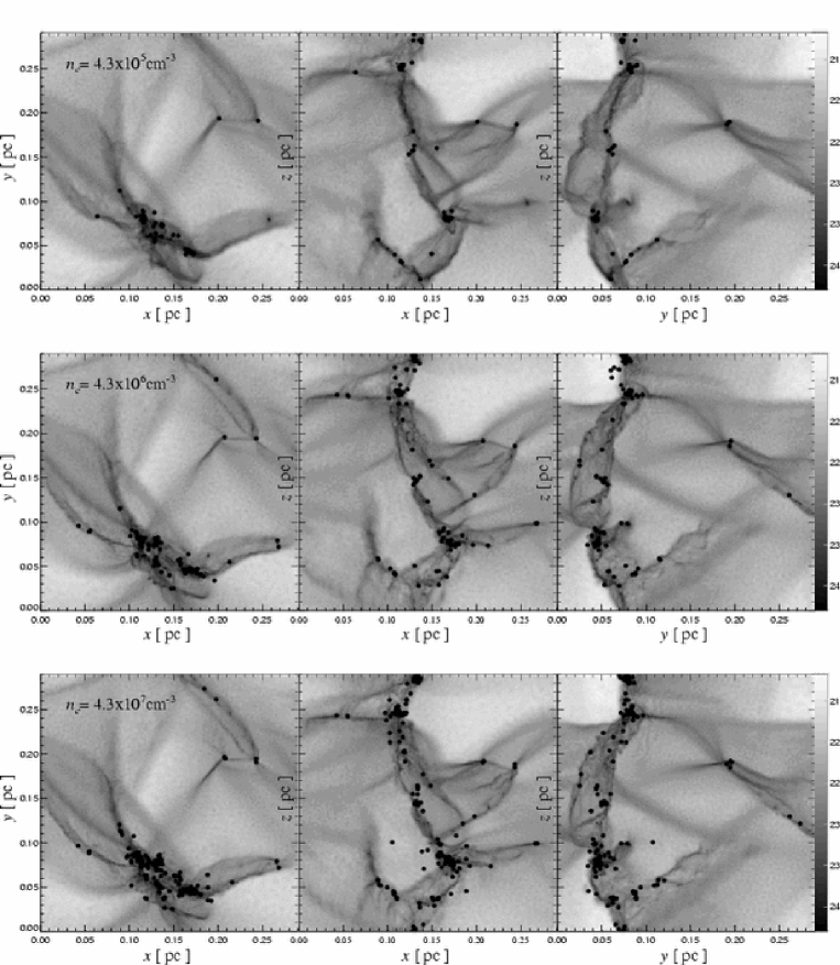
The filamentary structure that occurs in our simulations is visualized in Fig. 3. Here we show the column density distribution of the gas and the distribution of protostellar objects. We display the results for three different critical densities in xy-, xz- and yz-projection. The volume density is computed from the SPH kernel in 3D and then projected along the three principal axes. Figure 3 shows for all three cases a remarkably filamentary structure. These filaments define the loci where most protostellar objects form.

Clearly, the change of the polytropic exponent $\gamma$ at a certain critical density influences the number of protostellar objects. If the critical density increases then more protostellar objects form but the mean mass decreases.

We show this quantitatively in Fig. 4. In (a) we compare the number of protostellar objects for different critical densities $n_{\mathrm{c}}$ for the models R5…8k2b. The rate at which new protostars form changes with different $n_{\mathrm{c}}$. Models that switch from low $\gamma$ to high $\gamma$ at low densities built up protostellar objects more rarely than models that change $\gamma$ at higher densities.

Figure 4b shows the accretion histories (the time evolution of the combined mass fraction of all protostellar objects) for the models R5..8k2b. Accretion starts for all but one case approximately at the same time. In model R5k2b, $\gamma=1.1$ already at the mean initial density, thus $\gamma$ does not change during collapse. In this case accretion starts at a later time. This confirms the finding by Li et al. (2003) that accretion is delayed for large $\gamma$. In the other four cases the accretion history is very similar and the slope is approximately the same for all models.

In both plots we also show the results from our high resolution runs R7k2L and R8k2L. These simulations with 2 million and 5.2 million particles, respectively, have an accretion history similar to the time evolution of the accreted mass fraction in the runs with 1 million particles. The number of protostellar objects, however, is larger for the runs with increased particle numbers. Combining our results in these two figures we find that an environment where $\gamma$ changes at higher densities produces more, but less massive objects. Thus, the mean mass of protostellar objects does indeed depend on the critical density where $\gamma$ changes from 0.7 to 1.1.

6 Dependence of the characteristic mass on the equation of state

Figure 5: Mass spectra of protostellar objects for models R5..6k2b, model R7k2L and model R8k2L at $10\%$, $30\%$ and $50\%$ of total mass accreted on these protostellar objects. For comparison we also show in the first row the mass spectra of the isothermal run Ik2b. Critical density $n_{\mathrm{c}}$, ratio of accreted gas mass to total gas mass $M_{\mathrm{acc}}/M_{\mathrm{tot}}$ and number of protostellar objects are given in the plots. The vertical solid line shows the position of the median mass. The dotted line has a slope of -1.3 and serves as a reference to the Salpeter value (Salpeter 1955). The dashed line indicates the mass resolution limit.

Further insight into how the characteristic stellar mass may depend on the critical density can be gained from the mass spectra of the protostellar objects, which we show in Fig. 5. We plot the mass spectra of models R5…6k2b, model R7k2L and model R8k2L at different times, when the fraction of mass accumulated in protostellar objects has reached approximately $10\%,30\%$ and $50\%$. In the top row we also display the results of an isothermal run for comparison. We used the same initial conditions and parameters in all models shown. Dashed lines indicate the specific mass resolution limits.

We find closest correspondence with the observed IMF (see, Scalo 1998; Kroupa 2002; Chabrier 2003) for a critical density of $4.3\times 10^{6}\,\mathrm{cm^{-3}}$ and for stages of accretion around $30\%$ and above. At high masses, our distribution follows a Salpeter-like power law. For comparison we indicate the Salpeter slope $x\approx 1.3$ (Salpeter 1955) where the IMF is defined by $\mathrm{d}N/\mathrm{d}\log m\propto m^{-x}$. For masses about the median mass the distribution exhibits a small plateau and then falls off towards smaller masses.

The model R5k2b where the change in $\gamma$ occurs below the initial mean density, shows a flat distribution with only few, but massive protostellar objects. They reach masses up to $10\,M_{\odot}$ and the minimal mass is about $0.3\,M_{\odot}$. All other models build up a power-law tail towards high masses. This is due to protostellar accretion processes, as more and more gas gets turned into stars (see also, Bonnell et al. 2001b; Klessen 2001; Schmeja & Klessen 2004). The distribution becomes more peaked for higher $n_{\mathrm{c}}$ and there is a shift to lower masses. This is already visible in the mass spectra when the protostellar objects have only accreted $10\%$ of the total mass. Model R8k2L has minimal and maximal masses of $0.013\,M_{\odot}$ and $1.0\,M_{\odot}$, respectively. There is a gradual shift in the median mass (as indicated by the vertical line) from Model R5k2b, with $M_{\mathrm{med}}=2.5\,M_{\odot}$ at 50%, to Model R8k2L, with $M_{\mathrm{med}}=0.05\,M_{\odot}$ at 50%. A similar trend is noticeable during all phases of the model evolution.

This change of median mass with critical density $n_{\mathrm{c}}$ is depicted in Fig. 6. Again, we consider models R5…6k2b, model R7k2L and model R8k2L. The median mass decreases clearly with increasing critical density as expected. As we resolve higher density contrasts the median collapse mass decreases. We fit our data with a straight line. The slope takes values between $-0.4$ and $-0.6$. These values are larger than the slope $-0.95$ derived from the simple scaling law (Eq. 13) based on calculating the Jeans mass $M_{\mathrm{J}}$ at the critical density $n_{\mathrm{c}}$

One possible reason for this deviation is the fact that most of the protostellar objects are members of tight groups. Hence, they are subject to mutual interactions and competitive accretion that may change the environmental context for individual protostars. This in turn influences the mass distribution and its characteristics (see, e.g., Bonnell et al. 2001a, b). Another possible reason is that the mass that goes into filaments and then into collapse may depend on further environmental parameters, some of which we discuss in Sect. 7.

7 Dependence of the characteristic mass on environmental parameters

Figure 6: The plot shows the median mass of the protostellar objects over critical density for models R5..6k2b, model R7k2L and model R8k2L. We display results for different ratios of accreted gas mass to total gas mass $M_{\mathrm{acc}}/M_{\mathrm{tot}}$. We fit our data with straight lines for different stages of accretion. The slopes have the following values: $-0.43\pm 0.05$ (solid line), $-0.52\pm 0.06$ (dashed-dotted line), $-0.60\pm 0.07$ (dashed line).

7.1 Dependence on realization of the turbulent velocity field

We compare models with different realizations of the turbulent driving field in Fig. 7. We fit our data with straight lines for each stage of accretion. Figure 7a shows the results of models R5..8k2 which were calculated with the same parameters but lower resolution than the models used for Fig. 6. As discussed in Sec. 5, although the number of protostellar objects changes with the number of particles in the simulation, the time evolution of the total mass accreted on all protostellar objects remains similar. Thus, lower resolution models exhibit the same general trend as their high-resolution counterparts and show the same global dependencies. We notice, however, that the slope of the $M_{\mathrm{median}}$-$n_{\mathrm{c}}$ relation typically is shallower in the low-resolution models. This can be seen when comparing Fig. 6 and Fig. 7a, where we used identical turbulent driving fields.

For all four different realizations of the turbulent driving field shown in Fig. 7a-d we see a clear trend of decreasing median mass $M_{\mathrm{median}}$ with increasing $n_{\mathrm{c}}$. We conclude that, qualitatively, the $M_{\mathrm{median}}$-$n_{\mathrm{c}}$ relation is independent of the details of the turbulent driving field but, quantitatively, there are significant variations. This is not surprising given the stochastic nature of turbulent flows. A further discussion on this issue can be found in Klessen et al. (2000) and Heitsch et al. (2001).

Figure 7: Median mass of protostellar objects over critical density at different evolutionary phases (ratio of accreted gas mass over total gas mass $M_{\mathrm{acc}}/M_{\mathrm{tot}}$:10$\%$ (circle), 30$\%$ (star), 50$\%$ (triangle), 70$\%$ (square)). In (a)-(d) we show identical models but with different turbulent velocity fields (same root-mean-square velocity). The model in (e) is driven on a smaller scale $k=7..8$ than in the other cases. All relevant parameters are summarized in Table 1. We fit the median values with straight lines for different stages of accretion. The slopes are given in the plot and denoted as follows: 10$\%$ – solid line, 30$\%$ – dashed-dotted line, 50$\%$ – dashed line, 70$\%$ – dashed-double-dotted line.

7.2 Dependence on the scale of turbulent driving

Figure 7e shows the results for models where the driving scale has been changed to a lower value ($k=7..8$). The overall dependency of $M_{\mathrm{median}}$ on $n_{\mathrm{c}}$ is very similar to the cases of large-scale turbulence. However, we note considerably larger uncertainties in the exact value of the slope. This holds especially for the phases where $30\%$ and $50\%$ of the total gas mass has been converted into stars. One of the reasons is lower statistics, i.e., for the smallest critical density only one protostellar object forms. Moreover, it has already been noted by Li et al. (2003) that driving on small wavelength results in less fragmentation. The forming small-scale density structure is not so strongly filamentary, compared to the case of small-scale driven turbulence. Local differences have a larger influence on the results for driving on small wavelengths. Nevertheless, for most of the models the mean mass decreases with increasing critical density. Observational evidence suggests that real molecular clouds are driven from large scales (e.g. Ossenkopf & Mac Low 2002; Brunt et al. 2004).

8 Summary

Using SPH simulations we investigate the influence of a piecewise polytropic EOS on fragmentation of molecular clouds. We study the case where the polytropic index $\gamma$ changes from a value below unity to one above at a critical density $n_{\mathrm{c}}$. We consider a broad range of values of $n_{\mathrm{c}}$ around the realistic value to determine the dependence of the mass spectrum on $n_{\mathrm{c}}$.

Observational evidence predicts that dense prestellar cloud cores show rough balance between gravity and thermal pressure (Benson & Myers 1989; Myers et al. 1991). Thus, the thermodynamical properties of the gas play an important role in determining how dense star-forming regions in molecular clouds collapse and fragment. Observational and theoretical studies of the thermal properties of collapsing clouds both indicate that at densities below $10^{-18}\,\mathrm{g\,cm^{-3}}$, roughly corresponding to a number density of $n_{\mathrm{c}}=2.5\times 10^{5}\,\mathrm{cm^{-3}}$, the temperature decreases with increasing density. This is due to the strong dependence of molecular cooling rates on density (Koyama & Inutsuka 2000). Therefore, the polytropic exponent $\gamma$ is below unity in this density regime. At densities above $10^{-18}\,\mathrm{g\,cm^{-3}}$, the gas becomes thermally coupled to the dust grains, which then control the temperature by far-infrared thermal emission. The balance between compressional heating and thermal cooling by dust causes the temperature to increase again slowly with increasing density. Thus the temperature-density relation can be approximated with $\gamma$ above unity (Larson 1985) in this regime. Changing $\gamma$ from a value below unity to a value above unity results in a minimum temperature at the critical density. Li et al. (2003) showed that gas fragments efficiently for $\gamma<1.0$ and less efficiently for higher $\gamma$. Thus, the Jeans mass at the critical density defines a characteristic mass for fragmentation, which may be related to the peak of the IMF.

We investigate this relation numerically by changing $\gamma$ from $0.7$ to $1.1$ at different critical densities $n_{\mathrm{c}}$ varying from $4.3\times 10^{4}\,\mathrm{cm^{-3}}$ to $4.3\times 10^{7}\,\mathrm{cm^{-3}}$. A simple scaling argument based on the Jeans mass $M_{\mathrm{J}}$ at the critical density $n_{\mathrm{c}}$ leads to $M_{\mathrm{ch}}\propto n_{\mathrm{c}}^{-0.95}$. If there is a close relation between the average Jeans mass and the characteristic mass of a fragment, a similar relation should hold for the expected peak of the mass spectrum. Our simulations qualitatively support this hypothesis, however, with the weaker density dependency $M_{\mathrm{ch}}\propto n_{\mathrm{c}}^{-0.5\pm 0.1}$. The density at which $\gamma$ changes from below unity to above unity selects a characteristic mass scale. Consequently, the peak of the resulting mass spectrum decreases with increasing critical density. This spectrum not only shows a pronounced peak but also a powerlaw tail towards higher masses. Its behavior is thus similar to the observed IMF.

Altogether, supersonic turbulence in self-gravitating molecular gas generates a complex network of interacting filaments. The overall density distribution is highly inhomogeneous. Turbulent compression sweeps up gas in some parts of the cloud, but other regions become rarefied. The fragmentation behavior of the cloud and its ability to form stars depend strongly on the EOS. If collapse sets in, the final mass of a fragment depends not only on the local Jeans criterion, but also on additional processes. For example, protostars grow in mass by accretion from their surrounding material. In turbulent clouds the properties of the gas reservoir are continuously changing. In a dense cluster environment, furthermore, protostars may interact with each other, leading to ejection or mass exchange. These dynamical factors modify the resulting mass spectrum, and may explain why the characteristic stellar mass depends on the EOS more weakly than expected.

We also studied the effects of different turbulent driving fields and of a smaller driving scale. For different realizations of statistically identical large-scale turbulent velocity fields we consistently find the characteristic mass is decreasing with increasing critical mass. However, there are considerable variations. The influence of the natural stochastic fluctuations in the turbulent flow on the resulting median mass is almost as pronounced as the changes of the thermal properties of the gas. Also when inserting turbulent energy at small wavelengths we see the peak of the mass spectrum decreasing with increasing critical density.

Our investigation supports the idea that the distribution of stellar masses depends, at least in part, on the thermodynamic state of the star-forming gas. If there is a low-density regime in molecular clouds where temperature $T$ sinks with increasing density $\rho$, followed by a higher-density phase where $T$ increases with $\rho$, fragmentation seems likely to be favored at the transition density where the temperature reaches a minimum. This defines a characteristic mass scale. The thermodynamic state of interstellar gas is a result of the balance between heating and cooling processes, which in turn are determined by fundamental atomic and molecular physics and by chemical abundances. The derivation of a characteristic stellar mass can thus be based on quantities and constants that depend solely on the chemical abundances in a molecular cloud. The current study using a piecewise polytropic EOS can only serve as a first step. Future work will need to consider a realistic chemical network and radiation transfer processes in gas of varying abundances.

Appendix A Implementation of Sink Particles

The parallel version of GADGET distributes the SPH particles onto the individual processors, using a spatial domain decomposition. Thus, each processor hosts a rectangular piece of computational volume. If the position of a sink particle is near the boundary of this volume, the accretion radius overlaps with domains on other processors. We therefore communicate the data of the sink to all processors. Every processor searches for gas particles within the accretion radius of the sink. Three criteria determine whether the particle gets accreted or not. First, the particle must be bound to the sink particle, i.e., the kinetic energy must be less than the magnitude of the gravitational energy. Second, the specific angular momentum of the particle must be less than what is required to move on a circular orbit with radius $r_{\mathrm{acc}}$ around the sink particle. Finally, the particle must be more tightly bound to the candidate sink particle than to other sink particles. Once the central region of a collapsing gas clump exceeds a density contrast $\Delta\rho/\rho\sim 5000$, we introduce a new sink particle. The procedure for dynamically creating a sink particle is as follows. We search all processors for the gas particle with the highest density. When this density is above the threshold and when its smoothing length is less than half the accretion radius, then the gas particle is considered to become a sink particle. If the accretion radius around the candidate particle overlaps with another domain, its position is sent to the other processors. Every processor searches for the particles that exist in its domain and, simultaneously, within the accretion radius of the candidate particle. These particles and the candidate particle undergo a series of tests to decide if they should form a sink particle. First, the new sink particle must be the only one within two accretion radii. Second, the ratio of thermal energy to the magnitude of the gravitational energy must be less than 0.5. Third, we require that the total energy is less than zero. Finally, the divergence of the accelerations on the particles must be less than zero. If all these tests are passed, the particle with the highest density turns into a sink particle with position, velocity and acceleration derived from the center of mass values of the original gas particles. If these original particles are distributed over several processors the center of mass values have to be communicated correctly to the processor that hosts the new sink particle.

Ideally, the creation of sink particles in an SPH simulation should not affect the evolution of the gas outside its accretion radius. In practice there is the discontinuity in the SPH particle distribution due to the hole produced by the sink particles. This affects the pressure and viscous forces on particles outside. We have implemented adequate boundary conditions at the ”surface” of the sink particles as described in detail in Bate et al. (1995) to correct for these effects.

Following Bate et al. (1995) we use the Boss & Bodenheimer (1979) standard isothermal test case for the collapse and fragmentation of an interstellar cloud core to check our implementation. Initially, the cloud core is spherically symmetric with a small $m=2$ perturbation and uniformly rotating. As gravitational collapse proceeds a rotationally supported high-density bar builds up in the center embedded in a disk-like structure. The two ends of the bar become gravitationally unstable, resulting in the formation of a binary system. We see no further subfragmentation (see also, Truelove et al. 1997). These tests show that the precise creation time and the mass of the sink particle at the time of its formation can vary somewhat with the number of used processors. We also find that simulations with different processor numbers show small deviations in the exact positions and velocities of the gas particles. These variations are due to the differences in the extent of the domain on each processor. When the force on a particular particle is computed, the force exerted by distant groups is approximated by their lowest multipole moments. Since each processor constructs its own Barnes and Hut tree differences in the tree walk result in differences in the computed force. Hence, the formation mass and time of sink particles depend on the computational setup. Nevertheless, these differences are only at the $0.1\%$ level and the total number of collapsing objects is not influenced by a change in the number of processors.

References

- Adams & Fatuzzo (1996) Adams, F. C. & Fatuzzo, M. 1996, ApJ, 464, 256
- Arcoragi et al. (1991) Arcoragi, J., Bonnell, I., Martel, H., Bastien, P., & Benz, W. 1991, ApJ, 380, 476
- Basu & Mouschovias (1995) Basu, S. & Mouschovias, T. C. 1995, ApJ, 452, 386
- Bate et al. (1995) Bate, M. R., Bonnell, I. A., & Price, N. M. 1995, MNRAS, 277, 362
- Bate & Burkert (1997) Bate, M. R. & Burkert, A. 1997, MNRAS, 288, 1060
- Benson & Myers (1989) Benson, P. J. & Myers, P. C. 1989, ApJS, 71, 89
- Benz (1990) Benz, W. 1990, in Numerical Modelling of Nonlinear Stellar Pulsations Problems and Prospects, ed. J. R. Buchler (Dordrecht: Kluwer), 269
- Bodenheimer (1995) Bodenheimer, P. 1995, ARA&A, 33, 199
- Bodenheimer et al. (2000) Bodenheimer, P., Burkert, A., Klein, R. I., & Boss, A. P. 2000, Protostars and Planets IV, ed. V. Mannings, A. P. Boss & S. S. Russell (Tucson: Univ. of Arizona Press), 675
- Bonnell (1994) Bonnell, I. A. 1994, MNRAS, 269, 837
- Bonnell et al. (2001a) Bonnell, I. A., Bate, M. R., Clarke, C. J., & Pringle, J. E. 2001a, MNRAS, 323, 785
- Bonnell et al. (2001b) Bonnell, I. A., Clarke, C. J., Bate, M. R., & Pringle, J. E. 2001b, MNRAS, 324, 573
- Boss (1993) Boss, A. P. 1993, ApJ, 410, 157
- Boss & Bodenheimer (1979) Boss, A. P. & Bodenheimer, P. 1979, ApJ, 234, 289
- Brunt et al. (2004) Brunt, C. M., Heyer, M. H., Zivkov, V., & Mac Low, M.-M. 2004, ApJ, submitted
- Chabrier (2003) Chabrier, G. 2003, PASP, 115, 763
- Chandrasekhar & Fermi (1953) Chandrasekhar, S. & Fermi, E. 1953, ApJ, 118, 116
- Curry (2002) Curry, C. L. 2002, ApJ, 576, 849
- Durisen et al. (2001) Durisen, R. H., Sterzik, M. F., & Pickett, B. K. 2001, A&A, 371, 952
- Elmegreen (1997a) Elmegreen, B. G. 1997a, ApJ, 480, 674
- Elmegreen (1997b) —. 1997b, ApJ, 486, 944
- Elmegreen (1999) —. 1999, ApJ, 515, 323
- Elmegreen (2000a) —. 2000a, ApJ, 539, 342
- Elmegreen (2000b) —. 2000b, MNRAS, 311, L5
- Elmegreen (2002) —. 2002, ApJ, 564, 773
- Elmegreen & Mathieu (1983) Elmegreen, B. G. & Mathieu, R. D. 1983, MNRAS, 203, 305
- Elmegreen & Scalo (2004) Elmegreen, B. G. & Scalo, J. 2004, ARA&A, 42, 211
- Evans (1999) Evans, N. J. 1999, ARA&A, 37, 311
- Evans et al. (2001) Evans, N. J., Rawlings, J. M. C., Shirley, Y. L., & Mundy, L. G. 2001, ApJ, 557, 193
- Fleck (1982) Fleck, R. C. 1982, MNRAS, 201, 551
- Fromang et al. (2002) Fromang, S., Terquem, C., & Balbus, S. A. 2002, MNRAS, 329, 18
- Galli et al. (2001) Galli, D., Shu, F. H., Laughlin, G., & Lizano, S. 2001, ApJ, 551, 367
- Hartmann (2002) Hartmann, L. 2002, ApJ, 578, 914
- Hayashi (1966) Hayashi, C. 1966, ARA&A, 4, 171
- Hayashi & Nakano (1965) Hayashi, C. & Nakano, T. 1965, Prog. Theor. Phys., 34, 754
- Heitsch et al. (2001) Heitsch, F., Mac Low, M.-M., & Klessen, R. S. 2001, ApJ, 547, 280
- Hillenbrand (1997) Hillenbrand, L. A. 1997, AJ, 113, 1733
- Hillenbrand & Hartmann (1998) Hillenbrand, L. A. & Hartmann, L. W. 1998, ApJ, 492, 540
- Jappsen & Klessen (2004) Jappsen, A.-K. & Klessen, R. S. 2004, A&A, 423, 1
- Jeans (1902) Jeans, J. H. 1902, Philos. Trans. R. Soc. London, A, 199, 1
- Kawachi & Hanawa (1998) Kawachi, T. & Hanawa, T. 1998, PASJ, 50, 577
- Klessen (2001) Klessen, R. S. 2001, ApJ, 556, 837
- Klessen et al. (2004) Klessen, R. S., Ballesteros-Paredes, J., Vazquez-Semadeni, E., & Duran-Rojas, C. 2004, ApJ, in press, astro-ph/0306055
- Klessen et al. (1998) Klessen, R. S., Burkert, A., & Bate, M. R. 1998, ApJ, 501, L205+
- Klessen et al. (2000) Klessen, R. S., Heitsch, F., & Mac Low, M.-M. 2000, ApJ, 535, 887
- Koyama & Inutsuka (2000) Koyama, H. & Inutsuka, S. 2000, ApJ, 532, 980
- Kroupa (2001) Kroupa, P. 2001, MNRAS, 322, 231
- Kroupa (2002) —. 2002, Science, 295, 82
- Larson (1969) Larson, R. B. 1969, MNRAS, 145, 271
- Larson (1973a) —. 1973a, MNRAS, 161, 133
- Larson (1973b) —. 1973b, Fundamentals of Cosmic Physics, 1, 1
- Larson (1981) —. 1981, MNRAS, 194, 809
- Larson (1985) —. 1985, MNRAS, 214, 379
- Larson (2003) —. 2003, Rep. Prog. Phys., 66, 1651
- Larson (2005) —. 2005, MNRAS, submitted, astro-ph/0412357
- Lejeune & Bastien (1986) Lejeune, C. & Bastien, P. 1986, ApJ, 309, 167
- Li et al. (2003) Li, Y., Klessen, R. S., & Mac Low, M.-M. 2003, ApJ, 592, 975
- Lin & Papaloizou (1996) Lin, D. N. C. & Papaloizou, J. C. B. 1996, ARA&A, 34, 703
- Low & Lynden-Bell (1976) Low, C. & Lynden-Bell, D. 1976, MNRAS, 176, 367
- Mac Low (1999) Mac Low, M.-M. 1999, ApJ, 524, 169
- Mac Low & Klessen (2004) Mac Low, M.-M. & Klessen, R. S. 2004, Rev. Mod. Phys., 76, 125
- Mac Low et al. (1998) Mac Low, M.-M., Klessen, R. S., Burkert, A., & Smith, M. D. 1998, Phys. Rev. Lett., 80, 2754
- Mac Low & Ossenkopf (2000) Mac Low, M.-M. & Ossenkopf, V. 2000, A&A, 353, 339
- Masunaga & Inutsuka (2000) Masunaga, H. & Inutsuka, S. 2000, ApJ, 531, 350
- Monaghan (1992) Monaghan, J. J. 1992, ARA&A, 30, 543
- Monaghan & Lattanzio (1991) Monaghan, J. J. & Lattanzio, J. C. 1991, ApJ, 375, 177
- Motte et al. (1998) Motte, F., André, P., & Neri, R. 1998, A&A, 336, 150
- Murray & Lin (1996) Murray, S. D. & Lin, D. N. C. 1996, ApJ, 467, 728
- Myers (1978) Myers, P. C. 1978, ApJ, 225, 380
- Myers et al. (1991) Myers, P. C., Fuller, G. A., Goodman, A. A., & Benson, P. J. 1991, ApJ, 376, 561
- Myhill & Kaula (1992) Myhill, E. A. & Kaula, W. M. 1992, ApJ, 386, 578
- Nakano et al. (1995) Nakano, T., Hasegawa, T., & Norman, C. 1995, Ap&SS, 224, 523
- Ossenkopf et al. (2001) Ossenkopf, V., Klessen, R. S., & Heitsch, F. 2001, A&A, 379, 1005
- Ossenkopf & Mac Low (2002) Ossenkopf, V. & Mac Low, M.-M. 2002, A&A, 390, 307
- Padoan (1995) Padoan, P. 1995, MNRAS, 277, 377
- Padoan & Nordlund (2002) Padoan, P. & Nordlund, Å. 2002, ApJ, 576, 870
- Padoan et al. (1997) Padoan, P., Nordlund, A., & Jones, B. J. T. 1997, MNRAS, 288, 145
- Papaloizou & Lin (1995) Papaloizou, J. C. B. & Lin, D. N. C. 1995, ARA&A, 33, 505
- Passot & Vázquez-Semadeni (1998) Passot, T. & Vázquez-Semadeni, E. 1998, Phys. Rev. E, 58, 4501
- Penston (1969) Penston, M. V. 1969, MNRAS, 144, 425
- Price & Podsiadlowski (1995) Price, N. M. & Podsiadlowski, P. 1995, MNRAS, 273, 1041
- Salpeter (1955) Salpeter, E. E. 1955, ApJ, 121, 161
- Scalo (1998) Scalo, J. 1998, in ASP Conf. Ser. 142: The Stellar Initial Mass Function (38th Herstmonceux Conference), ed. G. Gilmore & D. Howell (San Francisco: Astron. Soc. Pac.), 201
- Scalo & Elmegreen (2004) Scalo, J. & Elmegreen, B. G. 2004, ARA&A, 42, 275
- Scalo et al. (1998) Scalo, J., Vazquez-Semadeni, E., Chappell, D., & Passot, T. 1998, ApJ, 504, 835
- Schmeja & Klessen (2004) Schmeja, S. & Klessen, R. S. 2004, A&A, 419, 405
- Schneider & Elmegreen (1979) Schneider, S. & Elmegreen, B. G. 1979, ApJS, 41, 87
- Shu (1977) Shu, F. H. 1977, ApJ, 214, 488
- Silk (1995) Silk, J. 1995, ApJ, 438, L41
- Silk & Takahashi (1979) Silk, J. & Takahashi, T. 1979, ApJ, 229, 242
- Spaans & Silk (2000) Spaans, M. & Silk, J. 2000, ApJ, 538, 115
- Springel et al. (2001) Springel, V., Yoshida, N., & White, S. D. M. 2001, New Astronomy, 6, 79
- Tafalla et al. (2004) Tafalla, M., Myers, P. C., Caselli, P., & Walmsley, C. M. 2004, A&A, 416, 191
- Tomisaka (1996) Tomisaka, K. 1996, PASJ, 48, 701
- Truelove et al. (1997) Truelove, J. K., Klein, R. I., McKee, C. F., et al. 1997, ApJ, 489, L179
- Turner et al. (1995) Turner, J. A., Chapman, S. J., Bhattal, A. S., et al. 1995, MNRAS, 277, 705
- Vázquez-Semadeni et al. (2005) Vázquez-Semadeni, E., Kim, J., Shadmehri, M., & Ballesteros-Paredes, J. 2005, ApJ, in press, astro-ph/0409247
- Whitworth & Summers (1985) Whitworth, A. & Summers, D. 1985, MNRAS, 214, 1
- Whitworth et al. (1995) Whitworth, A. P., Chapman, S. J., Bhattal, A. S., et al. 1995, MNRAS, 277, 727
- Wuchterl & Klessen (2001) Wuchterl, G. & Klessen, R. S. 2001, ApJ, 560, L185
- Zinnecker (1984) Zinnecker, H. 1984, MNRAS, 210, 43
- Zinnecker (1990) —. 1990, Physical Processes in Fragmentation and Star Formation, ed. R. Capuzzo-Dolcetta and C. Chiosi (Dordrecht: Kluwer), 201
- Zucconi et al. (2001) Zucconi, A., Walmsley, C. M., & Galli, D. 2001, A&A, 376, 650