Photometric Variability in the Faint Sky Variability Survey

L. Morales-Rueda,¹ P. J. Groot,¹ T. Augusteijn,² G. Nelemans,³ P. M. Vreeswijk,⁴ and E.J.M. van den Besselaar¹

Abstract

The Faint Sky Variability Survey (FSVS) is aimed at finding photometric and/or astrometric variable objects between 16th and 24th mag on time-scales between tens of minutes and years with photometric precisions ranging from 3 millimag to 0.2 mag. An area of $\sim$ 23 deg², located at mid and high Galactic latitudes, was covered using the Wide Field Camera (WFC) on the 2.5-m Isaac Newton Telescope (INT) on La Palma. Here we present some preliminary results on the variability of sources in the FSVS.

¹Department of Astrophysics, University of Nijmegen, P.O. Box 9010, 6500 GL Nijmegen, The Netherlands
²Nordic Optical Telescope, Ap. 474, 38700, La Palma, Spain
³Institute of Astronomy, Madingley Rd, CB3 0HA Cambridge, UK
⁴Astronomical Institute Anton Pannekoek, 1098 SJ Amsterdam, The Netherlands.

1. Introduction

The FSVS data set consists of 78 INT WFC fields. Each field is divided into four, corresponding to the 4 2kX4k CCDs that form the WFC. For each field, we took one set of B, I and V images on a given night. Several more images were taken in the V band on that night and on consecutive nights. Typically, fields were observed in V 10 – 20 times within one week. Exposure times were 10 min with a dead time between observations of 2 min. This observing pattern allows us to sample periodicity timescales from 2 $\times$ (observing time + dead time) (i.e. 24 min) up to the maximum time span of the observations (i.e. a few days). The combination of the colour information and the variability allows us to distinguish between different types of variable systems. See Groot et al. (2003) for a full discussion on the FSVS data.

2. The Floating Mean Periodogram

In order to combine the colour with the variability information contained in the FSVS we must be able to measure the variability timescale associated with each target. Because of the relatively few number of V observations per field (between 10 and 20) we use the “floating mean” periodogram technique to obtain the characteristic variability timescale in each case. This method has been used successfully in planet searches (Cumming et al. 1999) and to determine the orbits of subdwarf B binaries (Morales-Rueda et al. 2003).

The floating mean periodogram consists of fitting the data with a model composed of a sinusoid plus a constant of the form $\gamma+K\sin(2\pi f(t-t_{0})),$ where $f$ is the frequency and $t$ is the observation time. This method corrects a failing of the Lomb-Scargle periodogram (Lomb 1976; Scargle 1982) which subtracts the mean of the data and then fits a sinusoidal, which is incorrect for small numbers of points.

To test whether the periodogram was able to recover the correct periods, as a first step, we simulated the brightness variations of a series of sources with variability periods between 24 min and the time span of the observations, using the time sampling of one of the fields, and generated fake lightcurves for each period. We used the floating mean periodogram to calculate the most probable variability timescale of each lightcurve, and plotted the calculated versus the real period. The result is a linear curve with a 45^∘ slope (i.e. real periods are recovered successfully) and a complicated error structure. Examples of this test for two given variability amplitudes are presented in Fig. 1. Using a different time sampling (which is equivalent to analysing a different field) will generate a slightly different graph.

Refer to caption — Figure 1.: The variability timescale calculated using the floating mean periodogram is plotted versus the real variability timescale of data simulated using the time sampling of one of the FSVS fields. Data for two different variability amplitudes is presented.

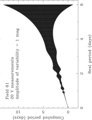
A more systematic and complete test to check that the method works, and to calculate its period detection efficiency, consists in generating curves like those of Fig. 1 for a complete range of values of variability timescale and amplitude, and object brightness (which is directly related to the uncertainty in the brightness measured for each band). These calculations must be done for each time sampling in the data (Morales-Rueda et al. in preparation).

3. Results

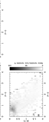
When we run the floating mean periodogram on the real data lightcurves we obtain their most likely variability timescale and the amplitude of that timescale. In the following colour-colour diagrams we show the point sources from the FSVS that show no variability (top left panel), the point sources that show variability (top right panel) and the ratio between variable and non-variable point sources (bottom panel). Variability is determined in each case by calculating the $\chi^{2}$ of the light curve with respect to its average value. Objects with $\chi^{2}$ above the 5- $\sigma$ variability level are considered variable (Groot et al. 2003). The ratio is presented in percentages. The main difference between the distribution of variable and non-variable objects is the excess of variable systems at colours B $-$ V $\sim$ 0 and V $-$ I $\sim$ 1. These sources will be mostly QSOs but we also expect any cataclysmic variables (CVs) in the field to appear in that colour-colour region. The fraction of variable to non-variable objects along the main sequence seems fairly uniform, but more rigorous calculations are required before we can draw any conclusions.

We also display the results in colour-colour diagrams for different ranges of variability timescales and amplitudes. The ranges have been selected so the first would include orbital periods corresponding to CVs (variability scales up to 6 hours), the second RR Lyr stars (scales from 6 hours to 1 day), the third longer variability trends of CVs (from 1 to 4 days), and anything else (above 4 days). Four different amplitude ranges are also chosen. In all colour-colour diagrams we have also plotted the 3- $\sigma$ upper limit of the main sequence for clarity. We find no obvious correlation between the time scales of the variability and their amplitudes.

In a preliminary analysis of the FSVS we find that, down to 24 mag, there are of the order of 500 objects in the variability range corresponding to CVs and 300 in the range corresponding to RR Lyr stars. We find 62 sources showing longer variability periods. The number of point sources found in each variability and amplitude range is given in Fig. 3. These preliminary values have not been corrected for the period detection efficiency discussed in Section 2 which might alter the results considerably.

Acknowledgments.

We thank T. R. Marsh for making his software available. The FSVS was supported by NWO Spinoza grant 08-0. The FSVS is part of the INT Wide Field Survey. LMR, EJMvdB and PJG are supported by NWO-VIDI grant 63g.ou2.201. The INT is operated on the island of La Palma by the Isaac Newton Group in the Spanish Observatorio del Roque de los Muchachos of the Instituto de Astrofísica de Canarias.

References

Cumming, A., Marcy, G.W., & Butler, R.P. 1999, ApJ, 526, 890

Groot, P.J., Vreeswijk, P.M., Huber, M.E., et al. 2003, MNRAS, 339, 427

Lomb, N.R., 1976, Ap&SS, 39, 447

Morales-Rueda, L., Maxted, P.F.L., Marsh, et al. 2003, MNRAS, 338, 752

Scargle, J.D., 1982, ApJ, 263, 835