On the Soft Excess in the X-ray Spectrum of Cir X–1: Revisitation of the Distance to Cir X–1

Abstract

We report on a 300 ks BeppoSAX (0.12–200 keV) observation of Circinus X–1 (Cir X–1) at phases between 0.62 and 0.84 and on a 90 ks BeppoSAX observation of Cir X–1 at phases 0.11–0.16. Using the canonical model adopted until now to fit the energy spectrum of this source large residuals appear below 1 keV. These are well fitted using an equivalent hydrogen column of $0.66\times 10^{22}$ cm^-2, adding absorption edges of O VII, O VIII and Ne IX in the spectra extracted from the observation at phases 0.62–0.84 and adding absorption edges of O VII, O VIII, Mg XI and Mg XII and absorption lines of O VIII and Mg XII in the spectra extracted from the observation at phases 0.11–0.16. During the observation at phases 0.62–0.84 the electron density associated to the ionized matter is $\sim 10^{13}$ cm^-3 remaining quite constant going away from the compact object. During the observation at phases 0.11–0.16 the electron density profile varies along the distance going from $\sim 6\times 10^{13}$ cm^-3 at $\sim 10^{11}$ cm to $\sim 9\times 10^{10}$ cm^-3 at $\sim 10^{13}$ cm. The equivalent hydrogen column towards Cir X–1 is three times lower than the value obtained from previous models. This low value would imply that Cir X–1 is at a distance of 4.1 kpc.

1 Introduction

Cir X–1 is a peculiar Low Mass X-ray Binary (LMXB), which recently showed ultra-relativistic outflows similar to those produced by active galactic nuclei (Fender et al. 2004). Because of its rapid variability, a black hole was supposed to be the compact object in this system (Toor 1977) until type I X-ray bursts were detected (Tennant et al. 1986a, 1986b), suggesting that the compact object is a neutron star.

Until 2002 Cir X–1 was supposed to be a runaway binary because of its supposed association with the supernova remnant G321.9-0.3 (Clark et al. 1975) at a distance between 5.5 kpc and 6.5 kpc (Case & Bhattacharya, 1998; Stewart et al. 1993). However, the work of Mignani et al. (2002), using HST data, excluded the association of Cir X–1 with G321.9-0.3. This brings to a new debate about the distance to Cir X–1. From the observed 21-cm absorption features in the radio spectrum of the source a lower limit to the distance of 6.4–8 kpc was obtained (Goss & Mebold, 1977; Glass, 1994). Generally in LMXBs the companion star has a mass $\lesssim 1$ M_⊙ and the orbit is almost circular; contrarily the canonical scenario accepted for Cir X–1 argues that the source has a companion star of $\sim 3-5$ M_⊙ (probably a subgiant, see Johnston et al. 1999), an orbital period of $\sim 16.6$ days, deduced from the radio and x-ray lightcurve of the source, and an eccentric orbit with $e\sim 0.7-0.9$ (Murdin et al. 1980; Tauris et al. 1999).

The correlated spectral and fast-timing properties of accreting low magnetic neutron stars allow distinguishing them into two classes, Z and atoll sources, using the pattern each source describes in an X-ray color-color diagram (Hasinger & van der Klis 1989). The Z sources are very bright and could have a moderate magnetic field ($<10^{10}$ Gauss), while the atoll sources have a lower luminosity and probably a weaker magnetic field. The timing analysis of RXTE data (Shirey et al. 1996) evidenced that Cir X–1 is more similar to LMXBs of the Z class. However no quasi periodic oscillations at kilohertz frequencies were observed in Cir X–1 (Shirey, 1996) contrarily to all the other Z-sources.

Cir X–1 also shows a peculiar X-ray spectrum. Brandt et al. (1996), using ASCA/GIS data taken in August 1994, found a sudden variation (in a timescale of $\sim 20$ minutes) of the flux at phase just after zero, where the count rate increased from $\sim 30$ counts s^-1 to $\sim 300$ counts s^-1. In the low-count rate state they obtained a good fit to the 0.6–10 keV spectrum of Cir X–1 using a partial covering component, in addition to a two-blackbody model, with a corresponding hydrogen column of $\sim 10^{24}$ cm^-2 and an intrinsic absorption of $\sim 1.7\times 10^{22}$ cm^-2; in the high-count rate state the partial covering of the X-ray spectrum was not needed. Because of the similarity with the spectra of Seyfert 2 galaxies with Compton-thin tori, Brandt et al. (1996) suggested that matter at the outer edge of the accretion disk, together with an edge-on disc orientation, could explain the partial covering of the spectrum of Cir X–1 (see, however, Fender et al. 2004).

Iaria et al. (2001a, 2002), using BeppoSAX data, analysed the 0.1–100 keV spectrum of Cir X–1 at phases 0.11–0.16 and 0.61–0.63. They found that the continuum could be well described by a Comptonization model at phases 0.11–0.16 and by the combination of a blackbody plus a Comptonization model at phases 0.61–0.63; the blackbody component is probably produced in the inner region of the accretion disc, while the Comptonized component is produced by a (hotter) corona surrounding the neutron star. A hard excess, dominanting the spectrum at energies higher than 15 keV, was also observed in both the observations and fitted by a power-law or a bremsstrahlung component. A similar feature was observed in other Z-sources (GX 17+2, Di Salvo et al. 2000; GX 349+2, Di Salvo et al. 2001; GX 5–1, Asai et al. 1994; Sco X–1, D’Amico et al. 2000; Cyg X–2, Di Salvo et al. 2002), suggesting that Cir X–1 shows a behavior similar to that of other Z-sources. Finally a strong absorption edge at $\sim 8.4-8.7$ keV, produced by highly ionized iron, was needed to fit the spectrum of Cir X–1 at phases 0.11–0.16.

The presence of a hard power-law component was recently confirmed by RXTE (3–200 keV) observations of Cir X–1 (Ding et al. 2003). They extracted the source spectra at different positions in the color-color diagram and concluded that there is no clear relation between the position of the source in the color-color diagram and the presence of the hard tail in the energy spectrum. An absorption edge, with energy ranging from 8.3 keV to 9.2 keV, was again observed, together with a localized emission feature present around 10 keV in the energy spectra corresponding to the normal branch and flaring branch; a similar feature was observed by Shirey et al. (1999). They interpret this line as produced by heavy elements, such as nickel, or, less probably, as a blue-shifted iron line due to the motion in a relativistic jet or to the rotation of the accretion disk; however extreme conditions would be required to boost the line energy up to 10 keV in this case.

Iaria et al. (2001b), using ASCA data, studied the energy spectrum of Cir X–1 along its orbit. They distinguished three different X-ray states of the source as a function of its phase. Therefore it was possible to study the evolution of the absorption edge along the orbit of Cir X–1. At the phase of the flaring activity, near the phase zero, the hydrogen column derived from the edge was $\sim 10^{24}$ cm^-2; at larger values of the phase the hydrogen column decreased; the absorption edge (from ionized iron) was no longer detected at phases from 0.78 to 1, while at these phases a partial covering component was required with an equivalent hydrogen column of $\sim 10^{24}$ cm^-2.

In general the X-ray spectrum of Cir X–1 is quite rich of discrete features. Brandt & Schulz (2000), using Chandra data, observed Cir X–1 near the phase zero. They found P-Cygni profiles of lines emitted by highly ionized elements. The outflow velocity necessary to explain the P-Cygni profiles was $\sim 2000$ km/s. Under the hypothesis that the source is seen nearly edge-on, they supposed that the model of a thermally driven wind (Begelman et al. 1983) could explain this outflow of ionized matter from the system. Also they suggested that the absorption edge observed by Iaria et al. (2001a) could be connected to the outflow.

The main point that should be clarified is the cycle of 16.6 days observed in the radio and X-ray lightcurve that was supposed to be the orbital period of the source. Just before the phase zero, associated to the radio outbursts, a dip is present in the x-ray folded lightcurve that was associated to the eclipse of the emitting source by the companion star. The long-term variability of the x-ray lightcurve and the large flaring activity, present near the phase zero, carried to the conclusion that Cir X–1 has an elliptical orbit with a large value of its eccentricity (Murdin et al., 1980) and that the phase zero corresponds to the periastron of the orbit. As noted by Clarkson et al. (2004) the dips are near-coincident with the presumed periastron passage suggesting that the semimajor axis of the binary orbit would have to be almost aligned with our line of sight to the binary system requiring an improbable fine tuning. Saz Parkinson et al. (2003), studying the RXTE/ASM lightcurve of Cir X–1 noted that the periodicity of 16.6 days is not always observed. They analysed the data from 6 Jan 1996 to 19 Sep 2002 finding that the cycle of 16.6 day is not present in a temporal interval lasting 270 days and that in this interval a new weak periodicity of 40 days is observed. If the cycle of 16.6 days is the orbital period of Cir X–1 is not easy to explain why during around 16 orbital periods the periodicity is no more observed while a new periodicity of 40 days appears. Then the results reported by Saz Parkinson et al. (2003) and Clarkson et al. (2004) seem to indicate that the cycle of 16.6 days in not connected to the orbital period of the binary system. Recently, from three radio observations Fender et al. (2004) resolve the structure of a jet in Cir X–1. The jet is extended up to 2.5 arcsec from the core. The authors, assuming a distance to the source of 6.5 kpc, find a superluminal motion of the jet having an apparent velocity of $v_{app}\simeq 15c$; because of the large value of the apparent velocity the angle between the line of sight and the direction of the jet, $\theta$, is $<5^{\circ}$ and the intrinsic velocity of the jet is $\beta>0.998$. The detection of the superluminal motion in the jet of Cir X–1 implies that $\theta<5^{\circ}$ and since the jet should have a direction almost perpendicular to the accretion disk it implies that Cir X–1 could not be an edge-on source contrarily to what was supposed until now.

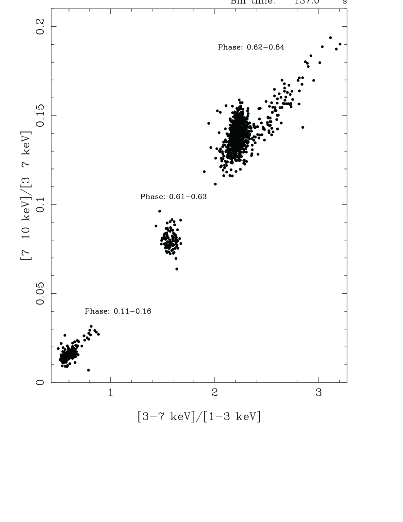
Figure 3: Color-color diagram of Cir X–1 of all the BeppoSAX observations (same as in Fig.2). The bin time is 137 s.

In this work we assume the ephemeris as reported by Stewart et al. (1991). We present the results of the analysis of the broad band (0.12–200 keV) spectra of Cir X–1 from a BeppoSAX observation taken at phases 0.62–0.84 in September 2001 and the reanalysis of the broad band spectrum of Cir X–1 from a previous BeppoSAX observation taken at phases 0.11–0.16 in August 1998 (see Iaria et al., 2001a). We note that, although the used model in that paper well fitted the data in the broad energy band 0.1–200 keV, a small bump in the residuals below 1 keV was present (see Fig. 3 in Iaria et al., 2001a). We will show that to well fit the data below 1 keV we need to add absorption edges of H-like and He-like ions of oxygen, neon and magnesium confirming the presence of highly ionized matter around the system. Moreover we discuss the possibility that Cir X–1 is distant 4.1 kpc implying that it does not show a super-Eddington luminosity as supposed until now.

The BeppoSAX observation of Cir X–1 at phases 0.61–0.63, already published by Iaria et al. (2002) and cited below in the text, will be not reanalysed because the available energy range for the spectral study is 1.8–200 keV, not allowing us to study the spectrum below 1 keV.

2 Observations

Two pointed observations of Cir X–1 were carried out in 2001 between Sep 08 00:47:57 UT and Sep 11 07:34:26 UT and in 1998 Aug 1 15:59:54.5 UT (this latter observation was already analyzed by Iaria et al., 2001a). The total exposure time was, respectively, 115 ks and 90 ks with the Narrow Field Instruments, NFIs, on board BeppoSAX (Boella et al. 1997). These consist of four co-aligned instruments covering the 0.1–200 keV energy range: a Low-Energy Concentration Spectrometer (LECS; operating in the range 0.1–10 keV), two Medium-Energy Concentration Spectrometers (MECS; 1.3–10 keV), a High-Pressure Gas Scintillation Proportional Counter (HPGSPC; 7–60 keV), and a Phoswich Detector System (PDS; 13–200 keV). We selected data from the LECS and MECS images in circular regions centered on the source with $8^{\prime}$ and $4^{\prime}$ radius, respectively. Data extracted from the same detector region during blank field observations were used for background subtraction. The background subtraction for the high-energy (non-imaging) instruments was obtained by using off-source data for the PDS and Earth occultation data for the HPGSPC. Assuming the ephemeris as reported by Stewart et al. (1991) the first observation covers the phase interval 0.62–0.84 and the second observation covers the phase interval 0.11–0.16.

In Figure 1 we plot the lightcurve of the observation at the phase interval 0.62–0.84 in the energy band 1.3–10 keV. The count rate smoothly decreases from $\sim 130$ counts s^-1, at the beginning of the observation, to $\sim 100$ counts s^-1, at 210 ks from the beginning of the observation. A flaring episode, lasting 50 ks, is present between 210 ks and 260 ks from the start time, the count rate varying from $\sim 100$ counts s^-1 to $\sim 190$ counts s^-1. The lightcurve of the observation in the interval phase 0.11–0.16 shows a large flare at the beginning of the observation lasting around 10 ks and the count rate increases from 300 counts s^-1 up to $\sim 700$ counts s^-1; after the flare the count rate varies in a range between 290 counts s^-1 and 400 counts s^-1 (see Fig. 1 in Iaria et al., 2001a).

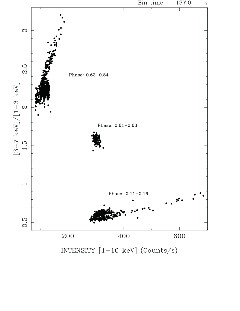
Figure 2: Hardness-intensity diagram of Cir X–1. We show in the same box the data at phase: 0.11-0.16 (Iaria et al. 2001a), the data at phase: 0.61-0.63 (Iaria et al. 2002), and the data at phase: 0.62-0.84 (this paper). The bin time is 137 s.

In Figure 2 we plot the hardness-intensity diagram, where the hardness ratio is the ratio between the count rate in the 3–7 keV energy band to the count rate in the 1–3 keV energy band, and the intensity is the count rate in the 1–10 keV energy band. In this figure we show the data of the two observations of this paper together with those of a previous BeppoSAX observation at phase 0.61–0.63 (see Iaria et al. 2002) taken in February 1999. The data of the observation at the interval phase 0.62–0.84 show a lower mean intensity of $\sim 120$ counts s^-1 and a larger hardness ratio than the data taken during the previous observation in the interval phase 0.61–0.63, which shows a count rate of $\sim 300$ counts s^-1 implying a decreasing of the flux of $\sim 60$%. In Figure 3 we plot the color-color diagram (CD), where the hard color (HC) is the ratio between the count rate in the energy band 7–10 keV to that in the energy band 3–7 keV and the soft color (SC) is the hardness ratio used for the hardness-intensity diagram. The data at phases 0.62–0.84 are at the top right in this figure while the data of the previous BeppoSAX observation at phases 0.61–0.63 show lower values of both the hard and the soft color. The CD indicates that the spectrum of Cir X–1, in the energy band 1–10 keV, is harder than those corresponding to the previous BeppoSAX observations.

To better see this long-term variation we checked the lightcurve of Cir X–1 taken by the All Sky Monitor (ASM) on board of the X–ray satellite RXTE. During the previous observation at the phase 0.61–0.63 (start time: 51216.14 MJD, stop time: 51217.80 MJD) the corresponding ASM count rate is $\sim 86$ counts s^-1, while during the observation analyzed here it is $\sim 36$ counts s^-1, implying that the flux decreased of 58%, in agreement with our BeppoSAX observations.

3 Spectral Analysis

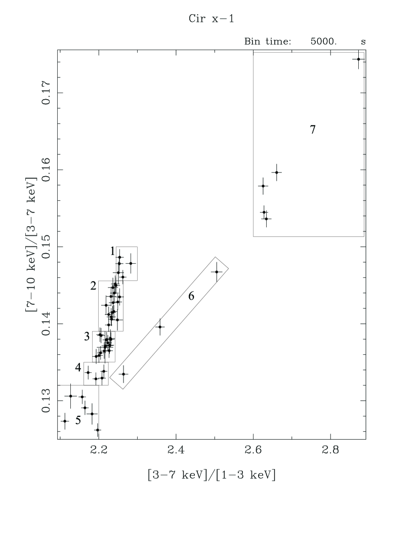
Figure 4: Color-color diagram of Cir X–1 corresponding to the observation at phases 0.62–0.84. The boxes indicate the seven selected zones from which we extracted the corresponding energy spectra. The bin time is 5 ks.

In Figure 4 we plot the CD of the observation corresponding to the interval phase 0.62–0.84. A bin time of 5 ks was adopted. The seven zones used to extract the corresponding energy spectra are indicated in the figure; zones 6 and 7 correspond to the flaring episode. In Tab. 1 we report the intervals of SC and HC which identify the seven selected zones, and the exposure times for each of the instruments. For each of the selected zones in the CD we extracted energy spectra for each instrument, which were rebinned in order to have at least 25 counts/energy-channel and to oversample the instrumental energy resolution with the same number of channels at all energies. A systematic error of 1% was added to the data. As customary, in the spectral fitting procedure we allowed for a different normalization of the LECS, HPGSPC and PDS spectra relative to the MECS spectrum, always checking that the derived values are in the standard range for each instrument. The energy ranges used for the spectral analysis are 0.12–4 keV for the LECS, 1.8–10 keV for the MECS, 7–30 for the HPGSPC and 15–200 keV for the PDS. We indicate the seven spectra with numbers from 1 to 7 corresponding to the seven selected zones in the CD.

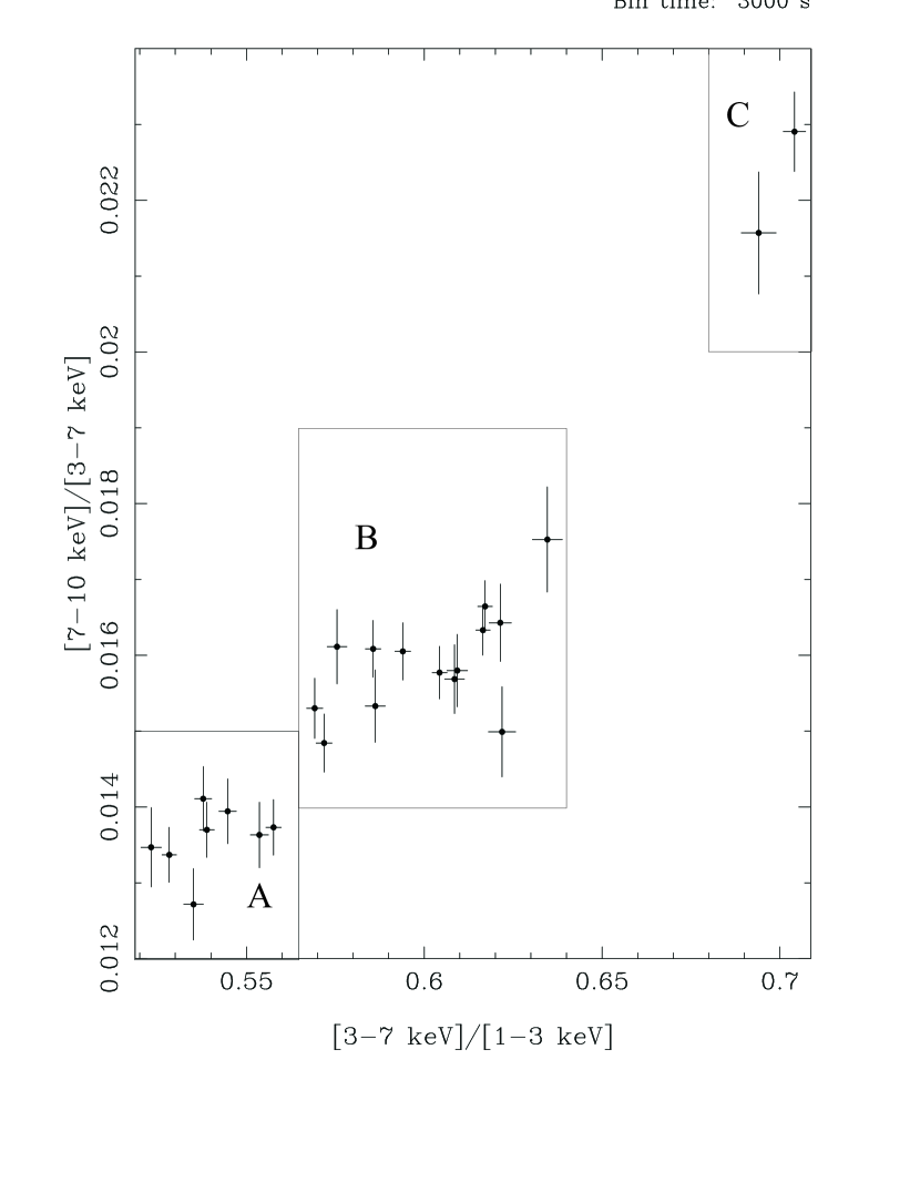
Figure 5: Color-color diagram of Cir X–1 corresponding to the observation at phases 0.11–0.16. The boxes indicate the selected regions from which we extracted the corresponding energy spectra. The bin time is 3 ks.

In Figure 5 we plotted the CD of the observation at phases 0.11–0.16. This observation was already studied by Iaria et al. (2001) which extracted from eight temporal intervals the corresponding energy spectra, grouping the data in order to have at least 20 counts/energy channel. In this paper we apply to the data the logarithmic grouping (in order to oversample to the instrumental energy resolution with the same number of channels at all energies) and a systematic error of 1%, instead of 2% as done in the previous analysis, (see e.g. Frontera et al., 2001). From the CD we selected three zones (see Fig. 5); the zone C corresponds to the flaring episode. In Tab. 2 we report the intervals of SC and HC which identify the three selected zones, and the exposure times for each of the instruments. We extracted energy spectra for each instrument from zone A and B because the zone C has not enough statistics. The spectra were extracted using the procedure described above. The energy ranges used for the spectral analysis are 0.12–2.85 keV for the LECS, 1.8–10 keV for the MECS, 7–30 for the HPGSPC and 15–200 keV for the PDS. We indicate the energy spectra with letters A and B corresponding, respectively, to the selected zones A and B in the CD.

3.1 The soft excess below 1 keV

To fit the seven spectra corresponding to the observation taken at phases 0.62–0.84 we used the Comptonization model Comptt (Titarchuk, 1994) to which we added a blackbody component at low energies in agreement with Iaria et al. (2002) who studied the source at similar phases. This model gave a $\chi^{2}/d.o.f.$ of 285/202, 364/200, 330/200, 254/201, 244/199, 249/199, and 256/200, respectively, for spectra 1 to 7; in Table 3 we show the corresponding best fit parameters. The equivalent absorption hydrogen column was $\sim 1.7\times 10^{22}$ cm^-2, the blackbody temperature around 0.55 keV, the seed-photon temperature and the electron temperature of the Comptonized component around 1 keV and 2.7 keV, respectively, and finally the optical depth, $\tau$, of the Comptonizing cloud is 11. The residuals obtained for the seven spectra are shown in Figure 6. The residuals corresponding to spectra 1, 2, 3 and 7 show a prominent soft excess reaching the maximum at 0.6–0.7 keV. The excess is less evident in spectra 4, 5 and 6, probably because of the lower statistics due to the lower LECS exposure times in these spectra (see Tab. 1).

To fit the spectra A and B (phases 0.11–0.16) we used the model proposed by Iaria et al. (2001a). The fits gave a $\chi^{2}/d.o.f.$ of 316/176 and 260/175, respectively for spectrum A and B. The residuals corresponding to the best fits are reported in Fig. 7. We note again the presence of a prominent soft excess in the residuals of both the spectra reaching the maximum at 0.6–0.7 keV similarly to those obtained from the spectra corresponding to the observation taken at phases 0.62–0.84. This soft excess is less prominent in spectrum B, again probably due to the lower statistics due to the lower LECS exposure time in spectrum B (see Tab. 2).

3.2 Fitting of the soft excess below 1 keV

To study the soft excess below 1 keV we start fitting the seven spectra corresponding to the observation taken at phases 0.62–0.84 because of the higher statistics (see Tabs. 1 and 2). Then we discuss several possible models, and finally we apply the best model to spectra A and B taken at phases 0.11–0.16.

Previous ASCA spectra of Cir X–1 were fitted using a partial covering component (Brandt et al., 1996; Iaria et al., 2001b). To compare our results with the previous ASCA results we fitted the seven spectra, in the energy range 1–10 keV, using only LECS and MECS data, with the model reported by Brandt et al. (1996). This model gave a $\chi^{2}/d.o.f.$ of 113/124, 119/124, 96/124, 95/124, 94/124, 104/124, and 103/124, respectively, for spectra 1 to 7. In agreement with Brandt et al. (1996) we find that the continuum emission is well fitted by two blackbody components absorbed by an equivalent hydrogen column of $\sim 1.7\times 10^{22}$ cm^-2. The partial covering component is present in the seven spectra, the equivalent hydrogen column, $N_{\rm H_{pc}}$, associated to this component is $\sim 2\times 10^{23}$ cm^-2 and the covered fraction of the emitting region is $\sim 0.3$. We applied the same model to our spectra using the energy range 0.12–10 keV taking into account the energy range where the soft excess is present. This model gave bad fits with a $\chi^{2}/d.o.f.$ of 252/164, 308/164, 373/164, 177/164, 198/164, 198/164, and 204/164, respectively, for spectra from 1 to 7, lefting unchanged the residuals below 1 keV. Finally we fitted the data in the whole energy range 0.12–200 keV using the continuum emission described in section 3.1 to which we added the partial covering component. We found that the spectrum above 1 keV is well fitted but the soft excess below 1 keV persists, implying that the soft excess cannot be fitted by a partial covering model. These results clearly show that the spectrum of Cir X–1 is more complex than it appeared in the energy band 1–10 keV.

We tried several emission components to fit this soft excess but no one gave reasonable results. The addition of an other blackbody component with a temperature of $\sim 0.15$ keV improved the fit, but the corresponding unabsorbed luminosity was $\sim 10^{42}$ erg/s in the 0.1–200 keV energy range. This result is very hard to explain assuming that the X–ray binary system contains a neutron star or a Galactic black hole. Instead of a blackbody we added a Gaussian line centered at 0.6 keV. Also in this case the results were not physically acceptable because, due to the high N_H, the corresponding equivalent width of the line was larger than 1 keV.

We conclude that the soft excess may have two possible origins: a) there is a continuum emission component below 1 keV absorbed by a lower value of equivalent hydrogen column with respect to the N_H absorbing the spectrum above 1 keV; b) the equivalent hydrogen column of the whole spectrum is overestimated.

As regards the first hypothesis, the residuals below 1 keV disappear if we add to the previous model a continuum emission component absorbed by a different lower equivalent hydrogen column (N${}_{H}\sim 8\times 10^{20}$ cm^-2) than that absorbing the other components of the model ($\sim 1.7\times 10^{22}$ cm^-2). However in this case it is hard to explain the lower value of N_H since the emitting source should be distant less than 1 kpc. Because in the LECS and MECS field of view no contaminating source is visible we should conclude that Cir X–1 is distant less 1 kpc or that a source with coordinates compatible with those of Cir X–1, at a distance less then 1 kpc, is present. Since this scenario looks unrealistic, in this paper we concentrate on the second hypothesis.

The second hypothesis would imply an equivalent hydrogen column, N_H, lower than $\sim 1.7\times 10^{22}$ cm^-2. A good fit of the broad band spectra is obtained adding two absorption edges at 0.7 keV and 1–1.2 keV having a large optical depth of $\sim 5$ and $\sim 1$ respectively. The threshold energy of the first absorption edge is similar in all the seven spectra while the threshold energy of the second absorption edge varies between 1 keV and 1.2 keV. Adding these features we find that the equivalent hydrogen column N_H is $\sim 0.6\times 10^{22}$ cm^-2 and the spectrum below 1 keV is well fitted.

In the residuals of spectra 2 and 3 a hard excess is present. In agreement with previous works (Iaria et al., 2001a; Iaria et al., 2002; Ding et al., 2003), we fitted it adding a power-law component having a photon index fixed to 2.6 in all the seven spectra. In spectra 6 and 7 a gaussian emission line, having its centroid at 6.7 keV, was needed. Two localized features are present at 7 keV and 9 keV in the seven spectra, we added two absorption edges to fit them. The residuals with respect to the final model are reported in Figure 8, the best fit parameters are reported in Table 4.

Because the structure of the residuals below 1 keV is the same in the spectra of both the observations presented in this work we fitted spectra A and B, corresponding to the observation taken at the phases 0.11–0.16, adding two absorption edges at 0.6 and 0.8 keV, in the model adopted by Iaria et al. (2001a). In this case the fits are improved adding two further absorption edges at 1.3 and 1.9 keV.

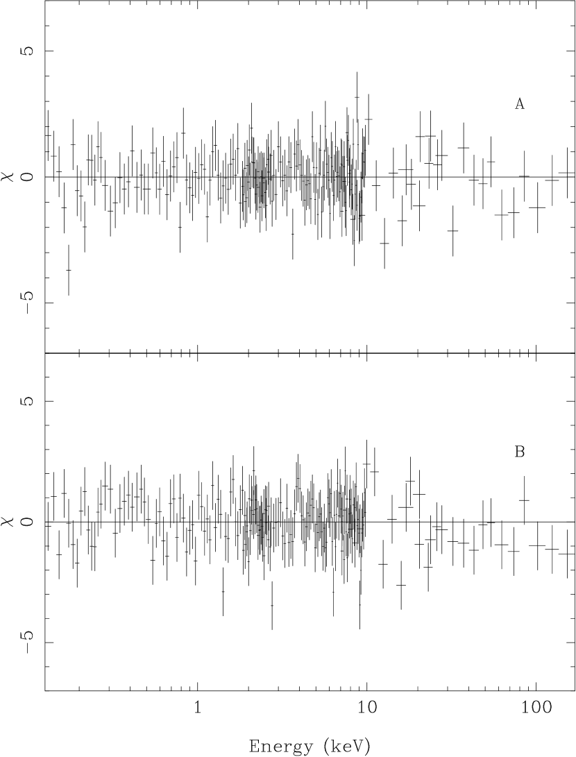
Figure 9: Residuals, in units of $\sigma$, of the spectra A e B corresponding to the observation at the phases 0.11–0.16. The residuals are with respect to the model reported in Tab. 5.

The parameters of these fits are reported in Tab. 5 and the residuals corresponding to the best-fits are plotted in Fig. 9. The addition of four absorption edges does not significantly change the parameters associated to the Comptonized component and the power-law component. The photon index of the power-law is fixed to 2.6 (as in spectra from 1 to 7). The equivalent hydrogen column is $\sim 0.6\times 10^{22}$ cm^-2, compatible with the values obtained from the other observation.

The poor LECS energy resolution and the low statistics below 1 keV do not allow us to well identify the absorption features at low energies. For this reason we fit the spectra from 1 to 7 fixing the equivalent hydrogen column to $0.66\times 10^{22}$ cm^-2 and the threshold energies of the absorption edges to those of O VII, O VIII and Ne IX. We use the same continuum model reported in Tab. 4. In Tab. 6 we report the best-fit parameters and in Fig. 10 we show the residuals with respect to this model. We note that the parameters of the continuum components are unchanged, and that we obtain good fits for all the seven spectra. Finally we fit the spectra A and B also fixing the equivalent hydrogen column to $0.66\times 10^{22}$ cm^-2 and the threshold energies of the absorption edges associated to O VII, O VIII, Mg XI and Mg XII. In this case two gaussian absorption lines associated to O VIII and Mg XII are added at $\sim 0.65$ keV and $\sim 1.47$ keV, respectively. Also in this case we find good fits, the best-fit parameters of the continuum are unchanged with respect to the model reported in Tab. 5; the new results are reported in Tab. 7 and the residuals are plotted in Fig. 11.

4 Discussion

We analyzed data of Cir X–1 from two BeppoSAX observations taken in September 2001 and August 1998 at phases 0.62–0.84 and 0.11–0.16 respectively.

About the observation at phases 0.62–0.84, taken in 2001, the lightcurve, the hardness-intensity diagram and the color-color diagram show that the intensity has decreased and soft and hard colors have increased with respect to previous observations at similar phases (0.61–0.63, Iaria et al. 2002). We selected seven zones in the color-color diagram and extracted from each of them the corresponding spectrum. The spectra, in the energy band 1–10 keV, are similar to that of other Z-sources (see Di Salvo et al. 2000; Di Salvo et al. 2001, Iaria et al. 2003), and are well fitted by a blackbody and a Comptonized component. Below 1 keV a soft excess is present in the residuals of spectra 1, 2, 3 and 7 (see Fig. 6); this can be fitted adding two absorption edges at 0.7 and 1 keV. The equivalent hydrogen column density, N_H, absorbing the continuum emission is $\sim 0.6\times 10^{22}$ cm^-2. In spectra 4, 5 and 6, where the soft excess is not evident, we fixed N_H to $0.6\times 10^{22}$ cm^-2 and added two absorption edges at low energies obtaining similar results. For this reason we conclude that in these spectra the absence of the soft excess below 1 keV is due to the lower statistics in the LECS data (see Tab. 1). However the poor LECS energy resolution and the low statistics below 1 keV do not allow us to well identify the absorption features at low energies. For this reason we fitted the spectra from 1 to 7 fixing the equivalent hydrogen column to $0.66\times 10^{22}$ cm^-2 and the threshold energies of the absorption edges to those of O VII, O VIII and Ne IX. In the following we will discuss this latter model.

About the observation at phases 0.11–0.16 taken in 1998, we reanalysed data already published by Iaria et al. (2001a) extracting the spectra from the corresponding color-color diagram while in the previous paper the spectra were extracted from eight temporal intervals along the entire observation. This allows to put in evidence the soft excess below 1 keV, only marginally visible in the previous analysis (see Fig. 3 in Iaria et al. 2001a). The continuum used to fit the data and the corresponding best-fit parameters are the same as reported by Iaria et al. (2001a). The addition of four absorption edges at 0.6 keV, 0.8 keV, 1.3 keV and 1.9 keV changes the equivalent absorption column that it is now $\sim 0.6\times 10^{22}$ cm^-2 instead of $\sim 1.7\times 10^{22}$ cm^-2 as reported in the previous paper. Also in this analysis, a prominent absorption edge at 8.4 keV and a Gaussian line at $\sim 6.7$ keV are present as already discussed by Iaria et al. (2001a). Also for this observation the poor LECS energy resolution and the low statistics below 1 keV do not allow us to well identify the absorption features at low energies. For this reason we fitted the spectra A and B fixing the equivalent hydrogen column to $0.66\times 10^{22}$ cm^-2 and the threshold energies of the absorption edges associated to O VII, O VIII, Mg XI and Mg XII. In this case two gaussian absorption lines associated to O VIII and Mg XII are added at $\sim 0.65$ keV and $\sim 1.47$ keV, respectively. In the following we will discuss this latter model.

This modeling was possible thanks to the good spectral coverage of the BeppoSAX/LECS, which gives us the possibility to study the X-ray spectrum down to 0.1 keV. For instance, recent Chandra observations (Brandt & Shulz 2000; Shulz & Brandt 2002) did not allow to well determine the continuum and the absorption features below 1 keV because the useful spectral range was limited to 1.4–7.3 keV. On the other hand, a K-shell absorption edge of neutral iron was observed in the two Chandra observations, although the choice to fix the hydrogen absorption column to $2\times 10^{22}$ cm^-2 might have influenced the value of the optical depth of the edge obtained from the fit. In a previous ASCA observation (Brandt et al. 1996) the estimated equivalent hydrogen column was N${}_{H}\sim 1.7\times 10^{22}$ cm^-2 similar to the value that we found not including the absorption edges at low energies (see Tab. 3). Note that the ASCA energy band used by Brandt et al. (1996) is 1–10 keV, which does not allow a clear detection of possible absorption edges at 0.7–1 keV. We confirm their results in the energy range 1–10 keV, where the spectrum is well fitted with an N${}_{H}\sim 1.7\times 10^{22}$ cm^-2 and where the K-shell absorption edge associated to neutral iron is fitted using a partial covering component. However, extending the energy range down to 0.1 keV this model does not fit the data below 1 keV.

4.1 The distance to Cir X–1

A source having the position of Cir X–1 and a distance to 5.5 kpc (Case & Battacharya 1998) has a corresponding visual extinction of $5.8\pm 2.0$ mag (Hakkila et al. 1997) and, using the observed correlation between visual extinction and equivalent hydrogen column (Predehl & Schmitt 1995), an equivalent hydrogen column N${}_{H}=(1.03\pm 0.02)\times 10^{22}$ cm^-2. In the previous ASCA (Brandt et al. 1996; Iaria et al. 2001b) and BeppoSAX (Iaria et al. 2001a; Iaria et al. 2002) observations an equivalent absorption column of $\sim 1.7\times 10^{22}$ cm^-2 was found and the authors concluded that an excess of obscuring matter was present close to the X-ray source. The value of the N_H obtained in this analysis is smaller than the previous one by a factor of three. The absorption we find (Tabs. 4 and 5) implies that for a source having the position of Cir X–1 the corresponding distance should be around 4 kpc.

If the interpretation of our data is correct the debate about the distance of Cir X–1 now becomes complicated. The N_H-based distance is not compatible with a distance between 6.4–8 kpc obtained from the 21-cm absorption features in the radio spectrum of the source (Goss & Mebold 1977; Glass 1994). Now we discuss this result using the latest estimate of the distance $R_{0}=8.5\pm 0.5$ kpc of the Galactic center from the Sun (Feast &Whitelock 1997) obtained using Hipparcos data.

Looking at the absorption H I spectrum in the direction of Cir X–1 (see figure 1 in Goss & Mebold 1977) five prominent radial velocities are present at 3.0, -6.5, -21.0, -57.5 and -75 km/s with a resolution of 0.82 km/s, the latter feature extends down to -90 km/s. Goss & Mebold (1977) observed in the direction of Cir X–1 seven times. The first observation was done when Cir X–1 was supposed not emitting in the radio band (Spectrum I) while three radio spectra, corresponding to three distinct observations, were averaged when the radio flux of Cir X–1 was around 1 Jy; Spectrum I was subtracted from the averaged spectrum. Supposing that no contaminating variable radio sources were present during the observations, the absorption line corresponding to the farthest H I cloud gives a lower limit to the distance to Cir X–1. Goss & Mebold (1977), assuming a distance to the center of our Galaxy R${}_{0}=10$ kpc and looking toward the direction of Cir X–1 at $l=322.117^{\circ}$ and $b=0.038^{\circ}$, obtained that the minimum distance between the Galactic center and the tangential point $R=R_{0}\sin l$ is 6.1 kpc and that the distance to the tangential point $d=R_{0}\cos l$ is 7.9 kpc. At the tangential point the radial velocity will be maximum, in our case $v_{r}=-88\pm 1$ km/s (see Figure 2 in Rohlfs et al. 1986). Since the radial velocity at -75 km/s extends up to -90 km/s and since -90 km/s is compatible with the radial velocity at the tangential point they assumed $d=7.9$ kpc as lower limit to the distance to Cir X–1. Rescaling these results using the most recent estimation of the distance to the Galactic center $R_{0}=8.5\pm 0.5$ (Feast & Whitelock, 1997), the lower limit to the distance of Cir X–1 should be $d=6.7\pm 0.4$ kpc. However we note that: a) although the radial velocity at -75 km/s extends down to -90 km/s the associated optical depth drastically decreases below 1 at -76 km/s becoming less prominent of the absorption line at 3 km/s (see fig. 1 in Goss & Mebold 1977); b) the absorption line at 3 km/s is produced by a cloud having a distance larger than the distance to the tangential point, implying that the lower limit to the Cir X–1 distance should be larger ($>13$ kpc, see Tab. 8) than that actually accepted. Note that the corresponding equivalent hydrogen column associated to a distance of 13 kpc is $\sim 3\times 10^{22}$ cm^-2, never observed in the X-ray spectra of Cir X–1. This suggests that possible contaminating radio sources are present during the observation. For these reason we analysed all the absorption lines present in the H I spectrum. To do it we used the following relation:

$$v_{r}=W(R)\sin l\cos b$$

$$R^{2}=R_{0}^{2}+d^{2}-2R_{0}d\cos l$$

(see Olling & Merrifield, 1998 and references therein). The function $W(R)$ is defined as $W(R)=R_{0}(\Omega(R)-\Omega_{0}(R_{0}))$, where $\Omega(R)$ is the angular speed of a celestial body around the Galactic center, $R$ the radius of the circular orbit and $\Omega_{0}(R_{0})$ is the angular speed of the local system of rest (LSR). Using the method of the tangential point, it is possible to write the function $W(R)$ as function of $R$ (see fig. 2 in Merrifield, 1992 and references therein); solving the two equations above we find the distances reported in Tab. 8.

In order to discriminate between these values we computed the corresponding visual extinction (Hakkila et al., 1997), the equivalent hydrogen column (Predehl & Schmitt 1995) and the proper motion $\mu$ (not corrected for the Solar motion) for each distance. These values are also reported in Tab. 8. Excluding the distances of 0.5 and 0.9 kpc, because the corresponding $N_{H}$ value is lower than that observed in the X–ray spectra of Cir X–1, we can give $d=4.1\pm 0.3$ kpc as a lower limit to the distance of Cir X–1. On the other hand we can exclude the distances 12.5 kpc, 12.9 kpc and 13.6 kpc because the corresponding $N_{H}$ values are larger than those observed in the X–ray spectra of Cir X–1. Using this argument the distance of the source should be in the range between $4.1\pm 0.3$ and $9.3\pm 0.6$ kpc. Our conclusion is in agreement with the results of $d>4$ kpc obtained by Whelan et al. (1977) using data in the optical band. Finally we note that a) a recent HST observation of the optical counterpart of Cir X–1 indicates that its proper motion (not corrected for the Solar motion) is $\mu=1.5\pm 1.6$ mas/yrs (Mignani et al., 2002) similar to the proper motion obtained for the lower limit of $d=4.1\pm 0.3$ kpc (see Tab. 8); b) the value of $N_{H}$ that we obtain from the fit in this work is around $0.6\times 10^{22}$ cm^-2 (see Tabs. 4 and 5), compatible with the value of $N_{H}$ obtained for $d=4.1\pm 0.3$ kpc. For this reason. in the following we will adopt a distance to Cir X–1 of 4.1 kpc, the corresponding value of $N_{H}$ will be $0.66\times 10^{22}$ cm^-2 (see Tab. 8) that is the same fixed in the fits reported in Tabs. 6 and 7.

This value of distance to Cir X–1 slightly changes the parameters associated to the radio jet observed from the source (Fender et al., 2004). From three radio observations Fender et al. (2004) resolved the structure of a jet in Cir X–1; the jet is extended up to 2.5 arcsec from the core. The authors, assuming a distance to the source of 6.5 kpc, find a superluminal motion of the jet with an apparent velocity of $v_{app}\simeq 15c$; because of the large value of the apparent velocity, the angle between the line of sight and the direction of the jet, $\theta$, is $<5^{\circ}$ and the intrinsic velocity of the jet is $\beta>0.998$. For a distance to Cir X–1 of 4.1 kpc, as we suggest, these values slightly change because now $v_{app}\simeq 9.2c$ implying $\theta<12^{\circ}$ and $\beta>0.995$. The extension of the jet of 2.5 arcsec corresponds to 0.12 light-years for 4.1 kpc, i.e. $1.1\times 10^{17}$ cm. The detection of the superluminal motion in the jet of Cir X–1 implies $\theta<12^{\circ}$ and, since the jet should have a direction almost perpendicular to the accretion disk, it confirms that Cir X–1 is not an edge-on source.

At the light of these results the mechanism producing the P-Cygni profiles from strongly ionized element, observed by Brandt & Shulz (2000) using a Chandra observation, should be rediscussed. The authors proposed a radiatively driven wind along the disk surface to explain the presence of these features in the Chandra grating spectra (see Brandt & Shulz, 2000; Shulz & Brandt 2002 for more details about their proposed model) but this mechanism could be valid only assuming that Cir X–1 is an edge-on source.

A possibility that should be investigate is that the ionized matter is ejected in a nearly perpendicular direction to the accretion disk surface.

4.2 The absorption features in the spectra and possible Reflection

In this section we discuss the absorption features reported in Tabs. 6 and 7 and obtained fixing the value of $N_{H}$ to $0.66\times 10^{22}$ cm^-2.

For the spectra from 1 to 7 the absorption edges associated to O VII, O VIII, Ne IX are probably produced in a plasma having a ionization parameter log${}_{10}\xi\sim 1.3$, for this value of $\xi$ the fractional number $f$ of O VII, O VIII, Ne IX of the corresponding elements is largest. We obtain the equivalent hydrogen column corresponding to the optical depth of the absorption edges using $\tau_{X}=\sigma_{X}N_{H}A_{X}f$, where $\sigma_{X}$ is the photoionization cross section for the ion X, $N_{H}$ is the corresponding equivalent hydrogen column, $A_{X}$ is the abundance of the element X and $f$ the fractional number of ions in the given ionization state of the considered element. The value of the photoionization cross sections are $2.4\times 10^{-19}$ cm², $9.9\times 10^{-20}$ cm² and $1.5\times 10^{-19}$ for O vii, O VIII and Ne IX, respectively (see Verner et al., 1996). Using the values of $\tau$ reported in Tab. 6, the cosmic abundance of oxygen and neon, and assuming an ionization parameters of log${}_{10}\xi=1.3$ (implying $f\sim 0.5$ for O VII, O VIII, Ne IX) we find that N${}_{H_{O\;VII}}$ $\sim 3\times 10^{22}$ cm^-2, N${}_{H_{O\;VIII}}$ $\sim 4\times 10^{22}$ cm^-2 and N${}_{H_{Ne\;IX}}$ $\sim 2\times 10^{22}$ cm^-2. We also observe an absorption edge probably associated to Fe XXV at 9 keV. The photoionization cross sections of Fe XXV is $2.0\times 10^{-20}$ cm² (see Verner et al., 1996). Assuming a ionization parameter log${}_{10}\xi$ of 3.3 (that implies the largest value of $f\sim 0.65$) we obtain that N${}_{H_{Fe\;XXV}}$ is $\sim 8.3\times 10^{22}$ cm^-2. In spectra 6 and 7 an emission line associated to Fe XXV is present. From $\xi=L_{x}/n_{e}r^{2}$ (see Krolik, McKee & Tarter, 1981) and $L_{line}=4\pi D^{2}I_{line}=n_{e}^{2}V\alpha Af$, we can obtain the distance, $r$, from the central source and the corresponding electron density, $n_{e}$, of the region where the line is produced. In the formulas $L_{x}$ is the total unabsorbed x-ray luminosity of the source in the energy band 0.12–200 keV, $L_{line}$ the luminosity of the line, $D$ the distance to the source, $I_{line}$ the intensity of the line, $V$ the emitting volume, $\alpha$ the recombination parameter, $A$ the cosmic abundance of iron. We assume a spherical volume $V$ of radius $r$ and, as written above, log${}_{10}\xi=3.3$ implies $f\sim 0.65$. The recombination parameter $\alpha$ is obtained using the relation and the best-fit parameters for H-like and He-like ions reported by Verner & Ferland (1996), where we fixed the plasma temperature at the electron temperature of the Comptonizing cloud; we find that the Fe XXV line is produced at $r\sim 2\times 10^{10}$ cm, with a corresponding electron density of $n_{e}\sim 7\times 10^{13}$ cm^-3. We can also estimate an upper limit to the distance to the emitting source, $d$, of the region where the absorption edges are produced. To do it we use $d<L_{x}/(N\xi)$ (Reynolds & Fabian, 1995), where $N$ is the equivalent hydrogen column associated to the photoionized matter, $d$ the distance to the central object, and $\xi$ and L_x are defined as above. We find that the O VII, O VIII and Ne IX absorption edges are produced at a distance to the central object of $d<5.3\times 10^{13}$ cm, and the Fe XXV absorption edge at $d<2.5\times 10^{11}$ cm. This latter distance is compatible with the distance associated to the Fe XXV absorption line.

In spectra A and B we fixed four absorption edges below 2 keV. The absorption edges associated to O VII, O VIII should be produced in a region having a lower ionization parameter (we assume log${}_{10}\xi=1$) with respect to the region where the absorption edges of Mg XI and Mg XII are produced (we assume log${}_{10}\xi=2.2$ for this latter region). For the spectra A and B we use a lower value of log${}_{10}\xi=1$ associated to O VII, O VIII than in the spectra from 1 to 7 because now we do not observe the Ne IX absorption edge.

Using the values of $\tau$ reported in tab. 7, the solar abundance of oxygen and assuming a ionization parameter log${}_{10}\xi$ of 1 (implying $f\sim 0.5$ for O VII and $f\sim 0.25$ for O VIII we find that N${}_{H_{O\;VII}}$ and N${}_{H_{O\;VIII}}$ are $\sim 4\times 10^{22}$ cm^-2. In the same way, knowing that the values of the photoionization cross sections of Mg XI and Mg XII are $1.0\times 10^{-19}$ cm² and $4.4\times 10^{-20}$ cm² respectively (see Verner et al., 1996) and assuming a ionization parameter log${}_{10}\xi$ of 2.2 (that implies the largest values of $f\sim 0.4$ for Mg XI and $f\sim 0.45$ for Mg XII), we obtain that N${}_{H_{Mg\;XI}}$ and N${}_{H_{Mg\;XII}}$ are $\sim 7\times 10^{22}$ cm^-2. An absorption edge probably associated to Fe XXIII is also present at 8.5 keV. The photoionization cross sections of Fe XXIII is $2.2\times 10^{-20}$ cm² (Krolik & Kallman, 1987). Assuming an ionization parameter log${}_{10}\xi$ of 2.9 (that implies the largest value of $f\sim 0.25$) we obtain that N${}_{H_{Fe\;XXIV}}$ is $\sim 4\times 10^{24}$ cm^-2, as already proposed by Iaria et al. (2001a). The upper limit to the distance of the region where this absorption edge is produced is $d<3.3\times 10^{10}$ cm.

Two absorption lines, associated to O VIII and Mg XII respectively, are present. The ionization parameter, log${}_{10}\xi$, associated to O VIII is 1 implying $f\sim 0.25$. We obtain that the O VIII absorption line is produced at $r\sim 1\times 10^{13}$ cm, with a corresponding electron density of $n_{e}\sim 9\times 10^{10}$ cm^-3. The ionization parameter , log${}_{10}\xi$, associated to Mg XII is 2.2 implying $f\sim 0.45$; we find that the Mg XII absorption line is produced at $r\sim 1\times 10^{11}$ cm, with a corresponding electron density of $n_{e}\sim 6.2\times 10^{13}$ cm^-3. On the other hand we find that the O VII and O VIII absorption edges are produced at $d<2.5\times 10^{14}$ cm, the Mg XI and Mg XII absorption edges are produced at $d<1\times 10^{13}$ cm. These upper limits are compatible with the distances derived for the O VIII and Mg XII absorption lines.

Finally an emission line at 6.7 keV is observed. Under the hypothesis that this is produced by Fe XXV we find that the distance and the electron density of the region producing this line are $r\sim 6\times 10^{11}$ cm and $n_{e}\sim 1.6\times 10^{11}$ cm^-3 respectively. This result is unrealistic because implies the presence of plasma with a ionization parameter of log${}_{10}\xi=3.3$ at a larger distance than the plasma having log${}_{10}\xi=2.2$, where the Mg XII absorption line is produced. A possible explanation is that the emission line at $\sim 6.7$ keV is associated to Fe XXIII; the corresponding centroid of the line should be $\sim 6.62$ keV and this does not change the results of the best fit for spectra A and B. In this case unfortunately we do not know the recombination parameter of the line and, consequently we cannot calculate the distance to the region where this line is produced.

Summarizing these results indicate that ionized matter is present around the system. During the observation at phases 0.62–0.84 this ionized matter could have an electron density quite constant along the distance of $\sim 7\times 10^{13}$ cm^-3; during the observation at phases 0.11–0.16 the electron density decreases going from the compact object to larger distances, varying between 9 $\times 10^{10}$ cm^-3 at 1 $\times 10^{13}$ cm and 6 $\times 10^{13}$ cm^-3 at 1 $\times 10^{11}$ cm. The different distribution of ionized matter along the distance from the neutron star, during the two observations, may influence the different observed continuum emission (see section 4.3). In Tab. 9 we summarize the obtained results.

Finally we observe an absorption edge associated to neutral iron in all the nine spectra. This feature was also observed during the Chandra observations (Brandt & Shulz, 2000; Shulz & Brandt, 2002). The optical depth is $\sim 0.05$ for spectra from 1 to 7 and less than $0.09$ in spectra A and B. Knowing that the cross section of the iron K-edge is $3.7\times 10^{-20}$ cm² we find that the equivalent hydrogen column associated to this feature is N${}_{H_{Fe\;I}}\sim 3\times 10^{22}$ cm^-2 and N${}_{H_{Fe\;I}}<5\times 10^{22}$ cm^-2 for the observation at phases 0.62–0.84 and 0.11–0.16, respectively. The estimated equivalent hydrogen column associated to the neutral iron is about 5 times higher than seen in the low-energy absorption indicating an overabundance of iron or special geometrical conditions. A plausible geometry was suggested by Singh & Apparao (1994) which found similar results for the Atoll source 4U 0614+09 analyzing EXOSAT data. The Fe I absorption edge is imprinted on the spectrum due to reflection by cold or partially ionized matter which is not in the same line of sight of the direct emission, therefore, lead to an estimate of N_H which is different from the value obtained from low-energy absorption.

4.3 The parameters of the continuum emission components

The model used to fit the data taken at the phases 0.62–0.84 is typical of the Z-sources (see Iaria et al., 2003 and references therein). It is composed by a blackbody plus a Comptonized component, and a power-law at energies above 10 keV. The corresponding radius of the blackbody component, assuming a spherical emission and a distance of 4.1 kpc is $\sim 20$ km. This radius is too large to be associated with the emission from the neutron star surface; therefore the blackbody component is probably emitted by the inner part of the accretion disk. Following in ’t Zand et al. (1999) we calculated the radius, $R_{W}$, of the seed-photon emitting region using the parameters reported in Table 6 and a distance to the source of 4.1 kpc; we obtain $R_{W}\sim 6$ km; this is smaller than the neutron star radius; a possible implication is that the electron cloud is not spherical. The continuum obtained at the phases 0.11–0.16 was already discussed by Iaria et al. (2001a), it is fitted by a very soft Comptonized component plus a power-law component, no blackbody emission is observed. In this case $R_{W}$ is $\sim 100$ km. In this case the shielding of the inner regions could be produced by a thicker optically region of the corona at inner radius. Assuming that the Comptonizing corona produces also the absorption feature observed in the spectra we deduce that during the observation at phases 0.62–0.84 the ionized matter has a low density allowing us to observe the inner region of the system up to 20 km from the compact object, while during the observation at phases 0.11-0.16 the density of the ionized matter is highest near the compact object forming a curtain that does not allow us to observe the inner region.

We also note that, although in the two observations considered in this paper the continuum emission below 10 keV is different, the spectra above 10 keV are fitted by a power-law component described by the same parameters, suggesting that its presence is independent of the phase and luminosity of the X-ray source. As described in other works (see Iaria et al., 2003 and references therein) it could be connected to the presence of a motion of relativistic electrons in a jet, as also suggested by Fender et al. (2004, see below).

The intrinsic total luminosity in the energy band 0.12–200 keV, L_x, is $\sim 4\times 10^{37}$ erg s^-1 during the observation at phases 0.62–0.84 and $\sim 1\times 10^{38}$ erg s^-1 during the observation at phases 0.11–0.16 for a distance to the source of 4.1 kpc.

5 Conclusions

In this work we present the analysis of the broad band (0.12–200 keV) spectrum of Cir X–1 at phases 0.62–0.84 and the reanalysis of the broad band (0.12–200 keV) spectrum of Cir X–1 at phases 0.11–0.16, using two BeppoSAX observations taken in 2001 and 1998 in respectively. In the spectra, a soft excess below 1 keV is observed using the model previously proposed. We fitted the soft excess using the equivalent hydrogen column of 0.66 $\times 10^{22}$ cm^-2 and adding at low energies absorption edges of O VII, O VIII, Ne IX, Mg XI and Mg XII. Moreover in the observation at phases 0.11-0.16 two absorption lines of O VIII and Mg XII were added.

The equivalent hydrogen column of the interstellar matter of $0.66\times 10^{22}$ cm^-2 gives a distance to Cir X–1 of 4.1 kpc. This result is discussed comparing it to the values obtained by Goss & Mebold (1977) and reanalyzing the HI spectrum of the source.

We discuss the different continuum observed in the two observations as due to the different density of the ionized matter around the binary system in the two observations.

Finally the reader should note that our results could be model dependent; for this reason further spectroscopic analysis of the Cir X–1 spectrum below 1 keV are need to confirm the scenario proposed in this work.

Table 1: BeppoSAX observation at phases 0.62-0.84. In columns 1 and 2 we show the intervals of Soft Color (SC) and Hard Color (HC) which identify the seven zones selected in the CD. In the other columns the corresponding exposure time, in ks, for each instrument is shown.

	SC	HC	LECS	MECS	HP	PDS
	Interval	Interval	ks	ks	ks	ks
1	2.24-2.30	0.145-0.15	4.7	8.7	7.0	3.4
2	2.20-2.26	0.139-0.145	7.7	32.0	28.3	14.1
3	2.18-2.24	0.135-0.139	9.7	32.1	47.6	14.9
4	2.16-2.22	0.132-0.135	2.0	8.9	8.8	4.3
5	2.08-2.2	0.124-0.132	1.9	11.9	11.4	4.7
6	2.24-2.26	0.124-0.176	1.9	5.1	4.0	1.4
7	2.6-2.9	0.124-0.176	4.8	10.5	8.6	9.9

Table 2: The same as in Tab. 1 for the BeppoSAX observation at phases 0.11-0.16.

	SC	HC	LECS	MECS	HP	PDS
	Interval	Interval	ks	ks	ks	ks
A	0.52-0.565	0.012-0.015	2.5	5.0	4.8	5.0
B	0.565-0.64	0.014-0.019	1.7	9.8	11.4	11.1
C	0.68-0.71	0.02-0.024	0	0.4	1.0	1.0

Table 3: Results of the spectral fits in the 0.12–200 keV energy band for the seven spectra corresponding to the observation taken at the phases 0.62–0.84. The photoelectric absorption is indicated as $N_{\rm H}$. The model is composed by a blackbody plus a Comptonized spectrum modeled by Comptt. Uncertainties are at 90% confidence level for a single parameter, upper limits are at 95% confidence level. $kT_{\rm BB}$ and N_BB are, respectively, the blackbody temperature and normalization in units of $L_{39}/D_{10}^{2}$, where $L_{39}$ is the luminosity in units of $10^{39}$ ergs/s and $D_{10}$ is the distance in units of 10 kpc. kT₀, kT_e and $\tau$ indicate the seed-photon temperature, the electron temperature and the optical depth of the Comptonizing cloud around the neutron star. N_comptt is the normalization of the Comptt model in XSPEC v.11.2.0 units.

Parameters	1	2	3	4	5	6	7
$N_{\rm H}$ $\rm(\times 10^{22}\;cm^{-2})$	$1.644^{+0.051}_{-0.049}$	$1.725^{+0.041}_{-0.040}$	$1.703^{+0.037}_{-0.036}$	$1.750^{+0.074}_{-0.070}$	$1.791^{+0.077}_{-0.072}$	$1.730^{+0.077}_{-0.074}$	$1.689^{+0.049}_{-0.048}$
kTBB (keV)	$0.549\pm 0.025$	$0.531\pm 0.017$	$0.537\pm 0.015$	$0.523\pm 0.024$	$0.505\pm 0.020$	$0.520\pm 0.022$	$0.550\pm 0.017$
NBB $(\times 10^{-2})$	$4.67\pm 0.28$	$4.77\pm 0.18$	$4.85\pm 0.17$	$4.87\pm 0.29$	$4.60\pm 0.26$	$4.51\pm 0.25$	$4.68\pm 0.17$
kT0 (keV)	$1.035\pm 0.040$	$1.034\pm 0.025$	$1.060\pm 0.023$	$1.019\pm 0.032$	$1.040\pm 0.030$	$1.187\pm 0.037$	$1.251\pm 0.028$
kTe (keV)	$2.820^{+0.038}_{-0.035}$	$2.796^{+0.026}_{-0.024}$	$2.725^{+0.026}_{-0.025}$	$2.751^{+0.038}_{-0.036}$	$2.704^{+0.061}_{-0.056}$	$2.678^{+0.091}_{-0.080}$	$2.715^{+0.058}_{-0.052}$
$\tau$	$11.93\pm 0.30$	$11.56\pm 0.21$	$11.28\pm 0.22$	$11.36\pm 0.29$	$10.70\pm 0.39$	$10.30\pm 0.62$	$10.43\pm 0.44$
Ncomptt	$1.071\pm 0.041$	$1.074^{+0.028}_{-0.027}$	$1.088^{+0.028}_{-0.026}$	$1.127^{+0.040}_{-0.041}$	$0.991\pm 0.041$	$1.109^{+0.054}_{-0.057}$	$1.256^{+0.039}_{-0.041}$
$\chi^{2}$ (d.o.f.)	285 (202)	364 (200)	330 (200)	254 (201)	244 (199)	249 (199)	256 (200)

Table 4: Parameters of the best fit model in the 0.12–200 keV energy band for the seven spectra corresponding to the observation taken at the phases 0.62–0.84. The continuum emission is fitted by a blackbody plus a Comptonized component (Comptt) and a power-law component. Uncertainties are at 90% confidence level for a single parameter, upper limits are at 95% confidence level. The power-law normalization, N_po, is in units of photons keV^-1 cm^-2 s^-1 at 1 keV. E${}_{edge_{1}}$ and E${}_{edge_{2}}$ are the energies of the two absorption edges, $\tau_{edge_{1}}$ and $\tau_{edge_{2}}$ their corresponding optical depths (see text). E${}_{\rm Fe\;{I}}$ and $\tau_{\rm Fe\;{I}}$ are the energy and the corresponding optical depth of the edge associated to neutral iron. E${}_{\rm Fe\;{XXV}}$ and $\tau_{\rm Fe\;{XXV}}$ are the energy and the corresponding optical depth of the edge associated to Fe xxv. E${}_{\rm Fe\;{\rm XXV}}$, $\sigma_{\rm Fe\;{\rm XXV}}$, I${}_{\rm Fe\;{\rm XXV}}$ and EQW${}_{\rm Fe\;{\rm XXV}}$ are, respectively, the centroid, width, intensity and equivalent width of the emission line at $\sim 6.7$ keV. I${}_{\rm Fe\;{\rm XXV}}$ is in units of photons cm^-2 s^-1. The other parameters are defined as in Tab. 3.

Parameters	1	2	3	4	5	6	7
$N_{\rm H}$ $\rm(\times 10^{22}\;cm^{-2})$	$0.57\pm 0.12$	$0.605^{+0.113}_{-0.085}$	$0.67\pm 0.13$	0.60 (fixed)	0.60 (fixed)	0.60 (fixed)	$0.45^{+0.16}_{-0.11}$
E${}_{edge_{1}}$ (keV)	$0.697^{+0.044}_{-0.031}$	$0.697^{+0.045}_{-0.032}$	$0.724^{+0.051}_{-0.041}$	$0.680^{+0.046}_{-0.064}$	$0.694^{+0.045}_{-0.079}$	$0.650^{+0.065}_{-0.430}$	$0.659^{+0.044}_{-0.039}$
$\tau_{edge_{1}}$	$5.6\pm 1.6$	$5.2\pm 1.8$	$5.13^{+1.71}_{-0.71}$	$8.0^{+2.9}_{-1.7}$	$7.4^{+2.4}_{-1.5}$	$5.4^{+2.8}_{-2.1}$	$6.3^{+2.9}_{-2.0}$
E${}_{edge_{2}}$ (keV)	$1.006\pm 0.079$	$0.955^{+0.096}_{-0.074}$	$1.025^{+0.177}_{-0.084}$	$1.209\pm 0.078$	$1.247\pm 0.079$	$0.962^{+0.079}_{-0.088}$	$0.978\pm 0.053$
$\tau_{edge_{2}}$	$0.90^{+0.78}_{-0.47}$	$1.23^{+1.08}_{-0.78}$	$0.66^{+0.75}_{-0.49}$	$0.38^{+0.20}_{-0.16}$	$0.28\pm 0.16$	$1.32^{+1.10}_{-0.85}$	$1.30^{+0.67}_{-0.52}$
E${}_{\rm Fe\;{\rm I}}$ (keV)	$7.08\pm 0.11$	$7.217^{+0.096}_{-0.074}$	$7.127^{+0.093}_{-0.087}$	$7.08\pm 0.13$	$7.103^{+0.096}_{-0.092}$	7.117 (fixed)	7.117 (fixed)
$\tau_{\rm Fe\;{\rm I}}$	$0.063\pm 0.019$	$0.056\pm 0.013$	$0.061\pm 0.013$	$0.055\pm 0.017$	$0.076\pm 0.017$	$0.031\pm 0.029$	$0.035\pm 0.020$
E${}_{\rm Fe\;{\rm XXV}}$ (keV)	$9.12\pm 0.21$	$8.96\pm 0.26$	$9.08^{+0.37}_{-0.28}$	$8.80\pm 0.18$	$8.96\pm 0.23$	$9.04\pm 0.48$	$8.91^{+0.28}_{-0.24}$
$\tau_{\rm Fe\;{\rm XXV}}$	$0.053\pm 0.019$	$0.051\pm 0.013$	$0.038\pm 0.013$	$0.064\pm 0.017$	$0.071\pm 0.019$	$0.036\pm 0.025$	$0.038\pm 0.017$
E${}_{\rm Fe\;{\rm XXV}}$ (keV)	–	–	–	–	–	$6.67^{+0.20}_{-0.11}$	$6.740^{+0.093}_{-0.051}$
$\sigma_{\rm Fe\;{\rm XXV}}$ (keV)	–	–	–	–	–	$<0.58$	$<0.23$
I${}_{\rm Fe\;{\rm XXV}}$ ($\times 10^{-3}$)	–	–	–	–	–	$4.5^{+2.5}_{-2.1}$	$3.2^{+1.7}_{-1.2}$
kTBB (keV)	$0.642^{+0.048}_{-0.053}$	$0.617\pm 0.037$	$0.611\pm 0.032$	$0.575\pm 0.052$	$0.567\pm 0.044$	$0.561\pm 0.052$	$0.613\pm 0.038$
NBB $(\times 10^{-2})$	$4.58\pm 0.81$	$4.26^{+0.54}_{-0.50}$	$4.47\pm 0.40$	$4.23^{+0.64}_{-0.55}$	$4.06^{+0.40}_{-0.36}$	$3.47^{+0.34}_{-0.39}$	$3.82\pm 0.36$
kT0 (keV)	$1.14\pm 0.12$	$1.099^{+0.073}_{-0.065}$	$1.138^{+0.060}_{-0.055}$	$1.048^{+0.088}_{-0.074}$	$1.090^{+0.077}_{-0.068}$	$1.183^{+0.097}_{-0.084}$	$1.295\pm 0.072$
kTe (keV)	$2.709^{+0.075}_{-0.066}$	$2.656^{+0.044}_{-0.041}$	$2.624^{+0.047}_{-0.043}$	$2.608^{+0.063}_{-0.057}$	$2.578^{+0.073}_{-0.067}$	$2.58\pm 0.11$	$2.664\pm 0.090$
$\tau$	$12.83\pm 0.76$	$12.69\pm 0.45$	$12.02\pm 0.45$	$12.58\pm 0.60$	$11.79\pm 0.69$	$11.2\pm 1.1$	$10.79\pm 0.86$
Ncomptt	$1.003^{+0.082}_{-0.077}$	$1.028\pm 0.055$	$1.039\pm 0.048$	$1.120\pm 0.079$	$0.974\pm 0.066$	$1.121^{+0.083}_{-0.086}$	$1.227^{+0.069}_{-0.076}$
Photon Index	2.60 (fixed)	2.60 (fixed)	2.60 (fixed)	2.60 (fixed)	2.60 (fixed)	2.60 (fixed)	2.60 (fixed)
Npo	$0.21\pm 0.15$	$0.208\pm 0.074$	$0.180\pm 0.065$	$0.18\pm 0.12$	$<0.05$	$<0.13$	$<0.16$
$\chi^{2}$ (d.o.f.)	203 (193)	246 (191)	222 (191)	189 (193)	182 (191)	198 (189)	161 (189)

Table 5: Parameters of the best fit model in the 0.12–200 keV energy band for the spectra A and B. The model is composed by a Comptonized component (Comptt) plus a power-law component. Uncertainties are at 90% confidence level for a single parameter, upper limits are at 95% confidence level. The parameters are defined as in Tab. 4.

Parameters	A	B
$N_{\rm H}$ $\rm(\times 10^{22}\;cm^{-2})$	$0.597^{+0.091}_{-0.088}$	$0.621^{+0.140}_{-0.078}$
E${}_{edge_{1}}$ (keV)	$0.624^{+0.042}_{-0.103}$	0.624 (fixed)
$\tau_{edge_{1}}$	$4.3^{+3.3}_{-1.3}$	$3.6\pm 1.7$
E${}_{edge_{2}}$ (keV)	$0.824^{+0.039}_{-0.034}$	$0.809\pm 0.034$
$\tau_{edge_{2}}$	$2.61^{+0.91}_{-0.97}$	$2.60\pm 0.81$
E${}_{edge_{3}}$ (keV)	$1.352\pm 0.029$	$1.303\pm 0.045$
$\tau_{edge_{3}}$	$0.145^{+0.048}_{-0.052}$	$0.118^{+0.028}_{-0.053}$
E${}_{edge_{4}}$ (keV)	$1.883\pm 0.025$	$1.870\pm 0.028$
$\tau_{edge_{4}}$	$0.128\pm 0.023$	$0.122^{+0.024}_{-0.027}$
E${}_{\rm Fe\;{\rm XXIII}}$ (keV)	$8.452\pm 0.058$	$8.467\pm 0.046$
$\tau_{\rm Fe\;{\rm XXIII}}$	$0.809^{+0.109}_{-0.088}$	$0.709^{+0.125}_{-0.081}$
E${}_{\rm Fe\;{\rm I}}$ (keV)	7.117 (fixed)	7.117 (fixed)
$\tau_{\rm Fe\;{\rm I}}$	$<0.070$	$<0.090$
E${}_{\rm Fe\;{\rm XXV}}$ (keV)	6.700 (fixed)	6.700 (fixed)
$\sigma_{\rm Fe\;{\rm XXV}}$ (keV)	$<0.25$	$<0.61$
I${}_{\rm Fe\;{\rm XXV}}$ $(\times 10^{-3})$	$1.18^{+0.55}_{-0.72}$	$1.86^{+1.42}_{-0.84}$
kT0 (keV)	$0.416^{+0.018}_{-0.015}$	$0.439\pm 0.019$
kTe (keV)	$0.933^{+0.065}_{-0.028}$	$0.997^{+0.091}_{-0.042}$
$\tau$	$14.09^{+0.71}_{-1.37}$	$13.7^{+1.1}_{-1.6}$
Ncomptt	$32.5^{+1.9}_{-4.3}$	$27.3^{+3.6}_{-4.7}$
Photon Index	2.60 (fixed)	2.60 (fixed)
Npo	$0.327\pm 0.063$	$0.228^{+0.054}_{-0.068}$
$\chi^{2}$ (d.o.f.)	184 (169)	214 (169)

Table 6: Parameters of the best fit model in the 0.12–200 keV energy band for the seven spectra corresponding to the observation taken at phases 0.62–0.84. The continuum emission is the same as reported in table 4. The absorption edges at low energies are interpreted as produced by ions of light elements and their corresponding optical depths are reported. Uncertainties are at 90% confidence level for a single parameter, upper limits are at 95% confidence level. Flux_BB, Flux_Comptt and Flux_po are the intrinsic fluxes in the energy band 0.12–200 keV, in units of $10^{-8}$ erg cm^-2 s^-1, of the blackbody, of the Comptonized component and of the power-law component, respectively. L_tot is the intrinsic total luminosity, in the energy band 0.12–200 keV, in units of erg s^-1 and assuming a distance to the source of 4.1 kpc.

Parameters	1	2	3	4	5	6	7
$N_{\rm H}$ $\rm(\times 10^{22}\;cm^{-2})$	0.66 (fixed)	0.66 (fixed)	0.66 (fixed)	0.66 (fixed)	0.66 (fixed)	0.66 (fixed)	0.66 (fixed)
E${}_{\rm O\;{\rm VII}}$ (keV)	0.739 (fixed)	0.739 (fixed)	0.739 (fixed)	0.739 (fixed)	0.739 (fixed)	0.739 (fixed)	0.739 (fixed)
$\tau_{\rm O\;{\rm VII}}$	$3.20^{+2.13}_{-0.93}$	$3.79^{+2.50}_{-0.93}$	$3.87^{+2.18}_{-0.92}$	$3.0^{+2.9}_{-1.1}$	$5.54^{+0.46}_{-2.38}$	$3.3^{+3.1}_{-1.3}$	$2.39^{+1.23}_{-0.70}$
E${}_{\rm O\;{\rm VIII}}$ (keV)	0.871 (fixed)	0.871 (fixed)	0.871 (fixed)	0.871 (fixed)	0.871 (fixed)	0.871 (fixed)	0.871 (fixed)
$\tau_{\rm O\;{\rm VIII}}$	$1.63^{+0.57}_{-1.30}$	$<2.09$	$<1.90$	$<2.41$	$<1.52$	$<2.51$	$2.05^{+0.48}_{-0.78}$
E${}_{\rm Ne\;{\rm IX}}$ (keV)	1.196 (fixed)	1.196 (fixed)	1.196 (fixed)	1.196 (fixed)	1.196 (fixed)	1.196 (fixed)	1.196 (fixed)
$\tau_{\rm Ne\;{\rm IX}}$	$0.16\pm 0.10$	$0.126\pm 0.085$	$0.168\pm 0.074$	$0.35\pm 0.15$	$0.31\pm 0.15$	$<0.17$	$<0.21$
E${}_{\rm Fe\;{\rm I}}$ (keV)	7.117 (fixed)	7.117 (fixed)	7.117 (fixed)	7.117 (fixed)	7.117 (fixed)	7.117 (fixed)	7.117 (fixed)
$\tau_{\rm Fe\;{\rm I}}$	$0.059\pm 0.018$	$0.052\pm 0.013$	$0.060\pm 0.013$	$0.054\pm 0.017$	$0.077\pm 0.017$	$0.038\pm 0.027$	$0.029\pm 0.019$
E${}_{\rm Fe\;{\rm XXV}}$ (keV)	$9.14\pm 0.21$	$8.87^{+0.25}_{-0.20}$	$9.07^{+0.36}_{-0.29}$	$8.81\pm 0.17$	$8.96\pm 0.22$	$9.02\pm 0.44$	$8.91^{+0.29}_{-0.25}$
$\tau_{\rm Fe\;{\rm XXV}}$	$0.050\pm 0.018$	$0.050\pm 0.012$	$0.036\pm 0.013$	$0.061\pm 0.017$	$0.071\pm 0.019$	$0.040\pm 0.025$	$0.036\pm 0.018$
E${}_{\rm Fe\;{\rm XXV}}$ (keV)	–	–	–	–	–	6.700 (fixed)	6.700 (fixed)
$\sigma_{\rm Fe\;{\rm XXV}}$ (keV)	–	–	–	–	–	$<0.44$	$<0.23$
I${}_{\rm Fe\;{\rm XXV}}$ ($\times 10^{-3}$)	–	–	–	–	–	$4.2^{+2.3}_{-1.9}$	$3.3^{+1.7}_{-1.3}$
EQW${}_{\rm Fe\;{\rm XXV}}$ (eV)	–	–	–	–	–	$30^{+17}_{-13}$	$19^{+10}_{-7}$
kTBB (keV)	$0.623^{+0.049}_{-0.052}$	$0.607\pm 0.035$	$0.604\pm 0.029$	$0.584\pm 0.048$	$0.575\pm 0.040$	$0.578^{+0.051}_{-0.048}$	$0.602\pm 0.037$
NBB $(\times 10^{-2})$	$4.49^{+0.78}_{-0.72}$	$4.36^{+0.48}_{-0.45}$	$4.50^{+0.38}_{-0.35}$	$4.39^{+0.62}_{-0.53}$	$4.10\pm 0.39$	$3.59^{+0.47}_{-0.40}$	$3.97^{+0.38}_{-0.34}$
RBB (km)	$20\pm 5$	$20\pm 3$	$21\pm 3$	$22\pm 5$	$22\pm 4$	$20\pm 5$	$20\pm 3$
FluxBB	$\sim 0.38$	$\sim 0.37$	$\sim 0.38$	$\sim 0.37$	$\sim 0.34$	$\sim 0.30$	$\sim 0.33$
kT0 (keV)	$1.110^{+0.110}_{-0.094}$	$1.102^{+0.066}_{-0.062}$	$1.138^{+0.055}_{-0.050}$	$1.065^{+0.084}_{-0.070}$	$1.099^{+0.072}_{-0.068}$	$1.207^{+0.096}_{-0.084}$	$1.285^{+0.073}_{-0.065}$
kTe (keV)	$2.710^{+0.060}_{-0.055}$	$2.686\pm 0.039$	$2.643^{+0.042}_{-0.040}$	$2.631^{+0.061}_{-0.057}$	$2.580^{+0.071}_{-0.068}$	$2.592^{+0.116}_{-0.094}$	$2.663^{+0.091}_{-0.082}$
$\tau$	$12.84\pm 0.63$	$12.48\pm 0.40$	$11.86\pm 0.40$	$12.38\pm 0.58$	$11.77^{+0.70}_{-0.66}$	$11.0\pm 1.1$	$10.82^{+0.79}_{-0.83}$
Ncomptt	$1.023\pm 0.076$	$1.028\pm 0.050$	$1.038\pm 0.044$	$1.100^{+0.071}_{-0.075}$	$0.966^{+0.065}_{-0.062}$	$1.103^{+0.080}_{-0.088}$	$1.237^{+0.065}_{-0.072}$
FluxComptt	$\sim 1.56$	$\sim 1.52$	$\sim 1.46$	$\sim 1.54$	$\sim 1.28$	$\sim 1.47$	$\sim 1.76$
RW (km)	$6\pm 1$	$6\pm 1$	$6\pm 1$	$7\pm 1$	$6\pm 1$	$6\pm 1$	$5\pm 1$
Photon Index	2.60 (fixed)	2.60 (fixed)	2.60 (fixed)	2.60 (fixed)	2.60 (fixed)	2.60 (fixed)	2.60 (fixed)
Npo	$0.19\pm 0.10$	$0.168\pm 0.061$	$0.139\pm 0.054$	$0.12\pm 0.11$	$<0.044$	$<0.44$	$<0.071$
Fluxpo	$\sim 0.18$	$\sim 0.16$	$\sim 0.13$	$\sim 0.11$	$<0.04$	$<0.41$	$<0.07$
Ltot $(\times 10^{37})$	$\sim 4.3$	$\sim 4.1$	$\sim 4.0$	$\sim 4.1$	$<3.4$	$<4.5$	$<4.3$
$\chi^{2}$ (d.o.f.)	210 (196)	254 (194)	224 (194)	187 (195)	182 (193)	205 (191)	176 (192)

Table 7: Parameters of the best fit model in the 0.12–200 keV energy band for spectra A and B. The model is defined in Tab. 5. We fixed the energies of the absorption edges present at low energies finding the corresponding optical depths. Uncertainties are at 90% confidence level for a single parameter, upper limits are at 95% confidence level. Fluxes are in units of $10^{-8}$ erg cm^-2 s^-1.

Parameters	A	B
$N_{\rm H}$ $\rm(\times 10^{22}\;cm^{-2})$	0.66 (fixed)	0.66 (fixed)
E${}_{\rm O\;{\rm VII}}$ (keV)	0.739 (fixed)	0.739 (fixed)
$\tau_{\rm O\;{\rm VII}}$	$4.22^{+1.07}_{-0.58}$	$4.17^{+1.10}_{-0.67}$
E${}_{\rm O\;{\rm VIII}}$ (keV)	0.871 (fixed)	0.871 (fixed)
$\tau_{\rm O\;{\rm VIII}}$	$0.76^{+0.43}_{-0.62}$	$<1.08$
E${}_{\rm Mg\;{\rm XI}}$ (keV)	1.762 (fixed)	1.762 (fixed)
$\tau_{\rm Mg\;{\rm XI}}$	$0.103^{+0.090}_{-0.038}$	$0.104\pm 0.36$
E${}_{\rm Mg\;{\rm XII}}$ (keV)	1.963 (fixed)	1.963 (fixed)
$\tau_{\rm Mg\;{\rm XII}}$	$0.052^{+0.059}_{-0.017}$	$0.048\pm 0.017$
E${}_{\rm Fe\;{\rm I}}$ (keV)	7.117 (fixed)	7.117 (fixed)
$\tau_{\rm Fe\;{\rm I}}$	$<0.094$	$<0.089$
E${}_{edge_{1}}$ (keV)	$8.447\pm 0.057$	$8.464\pm 0.041$
$\tau_{edge_{1}}$	$0.84^{+0.12}_{-0.10}$	$0.732^{+0.093}_{-0.080}$
E${}_{\rm O\;{\rm VIII}}$ (keV)	0.6537 (fixed)	0.6537 (fixed)
$\sigma_{\rm O\;{\rm VIII}}$ (keV)	$<0.34$	$<0.06$
I${}_{\rm O\;{\rm VIII}}$	$-1.36\pm 0.27$	$-1.24^{+0.29}_{-0.35}$
EQW${}_{\rm O\;{\rm VIII}}$ (eV)	$-125\pm 25$	$-135^{+33}_{-37}$
E${}_{\rm Mg\;{\rm XII}}$ (keV)	1.4726 (fixed)	1.4726 (fixed)
$\sigma_{\rm Mg\;{\rm XII}}$ (keV)	$<0.18$	$<0.08$
I${}_{\rm Mg\;{\rm XII}}$	$-0.171^{+0.075}_{-0.610}$	$-0.140^{+0.050}_{-0.097}$
EQW${}_{\rm Mg\;{\rm XII}}$ (eV)	$-19^{+8}_{-69}$	$-17^{+6}_{-12}$
E${}_{\rm Fe\;{\rm XXIII}}$ (keV)	6.62 (fixed)	6.62 (fixed)
$\sigma_{\rm Fe\;{\rm XXIII}}$ (keV)	$<0.31$	0.31 (fixed)
I${}_{\rm Fe\;{\rm XXIII}}$ $(\times 10^{-3})$	$1.12^{+0.64}_{-0.74}$	$1.75^{+0.81}_{-0.89}$
EQW${}_{\rm Fe\;{\rm XXIII}}$ (eV)	$29^{+18}_{-20}$	$39\pm 20$
kT0 (keV)	$0.430^{+0.015}_{-0.035}$	$0.447\pm 0.014$
kTe (keV)	$0.959^{+0.083}_{-0.052}$	$1.018^{+0.080}_{-0.054}$
$\tau$	$13.5^{+1.2}_{-1.6}$	$13.2^{+1.9}_{-3.0}$
Ncomptt	$29.5^{+2.8}_{-3.9}$	$25.9^{+1.9}_{-3.0}$
FluxComptt	$\sim 4.9$	$\sim 4.8$
RW (km)	$100\pm 20$	$90\pm 10$
Photon Index	2.60 (fixed)	2.60 (fixed)
Npo	$0.322\pm 0.065$	$0.219^{+0.055}_{-0.064}$
Fluxpo	$\sim 0.30$	$\sim 0.21$
Ltot $(\times 10^{38})$	$\sim 1.0$	$\sim 1.0$
$\chi^{2}$ (d.o.f.)	187 (170)	207 (170)

Table 8: In column 1 the radial velocities $v_{r}$ corresponding to the absorption features present in the HI spectrum of Cir X–1 are reported (see Goss & Mebold 1977); in column 2 the radius of the orbit of the clouds along the line of sight. In columns 3 the corresponding distances to the clouds of neutral matter. In columns 4 and 5 the visual extinction $A_{v}$ and the equivalent hydrogen column N_H corresponding to the distances; in column 6 the proper motion of the clouds. These values are calculated assuming a distance to the Galactic center of $8.5\pm 0.5$ kpc (Feast & Whitelock, 1997). The velocity at 3 km/s gives only one value of $d$ because its orbit has a radius larger than 8.5 kpc. (see text).

$v_{r}$	R	d	$A_{v}$	NH	$\mu$
km/s	kpc	kpc	mag	cm-2	mas/yrs
-75.0	$5.3\pm 0.3$	$5.9\pm 0.8$	$6.4^{+3.0}_{-2.5}$	$1.14\pm 0.21$	$0.4\pm 0.5$
		$7.6\pm 0.8$	$8.9^{+3.9}_{-3.2}$	$1.59\pm 0.24$	$-0.3\pm 0.3$
-57.5	$5.8\pm 0.4$	$4.1\pm 0.3$	$3.7\pm 1.4$	$0.66\pm 0.09$	$1.4\pm 0.3$
		$9.3\pm 0.6$	$11.4^{+4.3}_{-3.7}$	$2.04\pm 0.20$	$-0.6\pm 0.2$
-21	$7.8\pm 0.5$	$0.9\pm 0.1$	$0.73\pm 0.35$	$0.130\pm 0.005$	$5.5\pm 1.0$
		$12.5\pm 0.7$	$16.1^{+6.4}_{-5.5}$	$2.88\pm 0.23$	$-0.39\pm 0.06$
-6.5	$8.1\pm 0.5$	$0.5\pm 0.1$	$0.50^{+0.35}_{-0.30}$	$0.090\pm 0.016$	$3.3\pm 1.0$
		$12.9\pm 0.8$	$16.7^{+6.9}_{-5.9}$	$2.98\pm 0.26$	$-0.13\pm 0.02$
3.0	$8.6\pm 0.5$	$13.6\pm 0.8$	$17.7^{+7.6}_{-6.3}$	$3.17\pm 0.27$	$0.06\pm 0.02$

Table 9: Summary of the distance $d$, the electron densities $n_{e}$ and the equivalent hydrogen column $N$ associated to the ionized elements. $f$ and Log${}_{10}\xi$ are defined in the text.

Phases	O vii	O viii	O viii	Ne ix	Mg xi	Mg xi	Mg xii
0.62–0.84	edge	edge	line	edge	edge	edge	line
Log${}_{10}\xi$	1.3	1.3	–	1.3	–	–	–
$f$	0.5	0.5	–	0.5	–	–	–
d (cm)	$<5.3\times 10^{13}$	$<5.3\times 10^{13}$	–	$<5.3\times 10^{13}$	–	–	–
N (cm-2)	$\sim 3\times 10^{22}$	$\sim 4\times 10^{22}$	–	$\sim 2\times 10^{22}$	–	–	–
ne (cm-3)	–	–	–	–	–	–	–
Phase
0.11–0.16
Log${}_{10}\xi$	1.0	1.0	1.0	–	2.2	2.2	2.2
$f$	0.5	0.25	0.25	–	0.4	0.45	0.45
d (cm)	$<2.5\times 10^{14}$	$<2.5\times 10^{14}$	$\sim 1\times 10^{13}$	–	$<1\times 10^{13}$	$<1\times 10^{13}$	$\sim 1\times 10^{11}$
N (cm-2)	$\sim 4\times 10^{22}$	$\sim 4\times 10^{22}$	–	–	$\sim 7\times 10^{22}$	$\sim 7\times 10^{22}$	–
ne (cm-3)	–	–	$\sim 9.2\times 10^{10}$	–	–	–	$\sim 6.2\times 10^{13}$

Phases	Fe xxiii	Fe xxv	Fe xxv
0.62–0.84	edge	line	edge
Log${}_{10}\xi$	–	3.3	3.3
$f$	–	0.65	0.65
d (cm)	–	$\sim 2\times 10^{10}$	$<2.5\times 10^{11}$
N (cm-2)	–	–	$\sim 8.3\times 10^{22}$
ne (cm-3)	–	$n_{e}\sim 7\times 10^{13}$	–
Phase
0.11–0.16
Log${}_{10}\xi$	2.9	–	–
$f$	0.25	–	–
d (cm)	$<3.3\times 10^{10}$	–	–
N (cm-2)	$\sim 4\times 10^{24}$	–	–
ne (cm-3)	–	–	–

Figure 1: Cir X–1 lightcurve in the energy band 1.3–10 keV (MECS data). The data corresponding to the phase interval 0.62–0.84 assuming the ephemeris as reported by Stewart et al. (1991). The bin time is 550 s.

Figure 6: Residuals, in units of $\sigma$, of the seven spectra corresponding to the observation at the phases 0.62–0.84. The residuals are with respect to the model reported in Tab. 3.

Figure 7: Residuals, in units of $\sigma$, of the spectra A e B corresponding to the observation at the phases 0.11–0.16 with respect to the model adopted by Iaria et al. (2001a).

Figure 8: Residuals, in units of $\sigma$, of the seven spectra corresponding to the observation at the phases 0.62–0.84. The residuals are with respect to the model reported in Tab. 4.

Figure 10: Residuals, in units of $\sigma$, of the seven spectra corresponding to the observation at the phases 0.62–0.84. The residuals are with respect to the model reported in Tab. 6.

Figure 11: Residuals, in units of $\sigma$, of the two spectra corresponding to the observation at the phases 0.11–0.16. The residuals are with respect to the model reported in Tab. 7.

References

- (1) Anders, E., Grevesse, N., 1989, Geochimica et Cosmochimica Acta, 53, 197
- (2) Asai, K. et al. 1994, PASJ, 46, 479
- (3) Begelman, M. C., McKee, C. F., Shields, G. A., 1983, ApJ, 271, 70
- (4) Boella G., Butler R. C., Perola G. C., Piro L., Scarsi L., Blecker J., 1997, A&AS, 122, 299
- (5) Brandt, W. N., Fabian, A. C., Dotani, T., Nagase, F., Inoue, H., Kotani, T., Segawa, Y., 1996, MNRAS, 283, 1071
- (6) Brandt, W. N.; Schulz, N. S., 2000, ApJL, 544, L123
- (7) Clarkson W. I., Charles P. A., Onyett N., 2004, MNRAS, 348, 458
- (8) Case, G. L., Bhattacharya, D., 1998, ApJ, 504, 761
- (9) Clark, D. H., Parkinson, J. H., Caswell, J. L., 1975, Nature, 254, 674
- (10) D’Amico, F., Heindl, W. A., Rothschild, R. E., & Gruber, D. E., 2001, ApJ, 547, L147
- (11) Ding, G. Q., Qu, J. L., Li, T. P., 2003, ApJ, 596, 219
- (12) Di Salvo, T., et al. 2000, ApJ, L544, 119
- (13) Di Salvo, T., et al. 2001, ApJ, 554, 49
- (14) Feast M., Whitelock P., 1997, MNRAS, 291, 683
- (15) Fender R., Wu K., Johnston H. et al., 2004, Nature, 427, 222
- (16) Frontera F. et al., 2001, ApJ, 501, 1006
- (17) Glass, I. S., 1994, MNRAS, 268, 742
- (18) Goss, W. M., Mebold, U., 1977, MNRAS, 181, 255
- (19) Hakkila, J., Myers, J. M., Stidham, B. J., Hartmann, D. H., 1997, AJ, 114, 2043
- (20) Hasinger, G., & van der Klis, M., 1989, A&A, 225, 79
- (21) Iaria, R.; Burderi, L., Di Salvo, T., La Barbera, A., Robba, N. R., 2001a, ApJ, 547, 412
- (22) Iaria, R., Di Salvo, T., Burderi, L., Robba, N. R., 2001b, ApJ, 561, 321
- (23) Iaria, R., Di Salvo, T., Robba, N. R., Burderi, L., 2002, ApJ, 567, 503
- (24) Iaria, R., Di Salvo, T., Robba, N. R., Burderi, L., 2004, ApJ, 600, 358
- (25) in ’t Zand, J. J. M. et al. 1999, A&A, 345, 100
- (26) Johnston, H. M., Fender, R., Wu, K., 1999, MNRAS, 308, 415
- (27) Krolik, J. H., McKee, C. F., Tarter, C. B., 1981, ApJ, 249, 422
- (28) Krolik, J. H., Kallman, T. R., 1987, ApJL, 320, L5
- (29) Margon, B., Lampton, M., Bowyer, S., Cruddace, R., 1971, ApJL, 169, L23
- (30) Merrifield M. R., 1992, AJ, 103, 1552
- (31) Mignani, R. P., De Luca, A., Caraveo, P. A., Mirabel, I. F., 2002, A&A, 386, 487
- (32) Murdin, P., Jauncey, D. L., Haynes, R. F., Lerche I., Nicolson, G. D., Holt, S. S., Kaluzienski, L. J., 1980, A&A, 87, 292
- (33) Neckel, Th., Klare G., 1980, A&AS, 42, 251
- (34) Olling R. P., Merrifield M. R., 1998, MNRAS, 297, 943
- (35) Predehl, P., Schmitt, J. H. M. M., 1995, A&A, 293, 889
- (36) Reynolds C. S. & Fabian A. C., 1995, MNRAS, 273, 1167
- (37) Rohlfs K., Chini R., Wink J. E. et al., 1986, A&A, 158, 181
- (38) Saz Parkinson P. M., Tournear D. M., Bloom E. D., Focke W. B., Reilly K. T., 2003, ApJ, 595, 333
- (39) Shirey R. E., Bradt, H. V., Levine, A. M., Morgan, E. H., 1996, ApJL, 469, L21
- (40) Shulz, N. S., & Brandt, W. N., 2002, ApJ, 572, 971
- (41) Singh, K. P., Apparao, K., M., V., 1994, ApJ, 431, 826
- (42) Stewart, R. T., Nelson, G. J., Penninx, W., Kitamoto, S., Miyamoto, S., Nicolson, G. D., 1991, MNRAS, 1991, 253
- (43) Stewart, R. T., Caswell, J. L., Haynes, R. F., Nelson, G. J., 1993, MNRAS, 261, 593
- (44) Tauris, T. M., Fender, R. P., van den Heuvel, E. P. J., Johnston, H. M., Wu, K., 1999, MNRAS, 310, 1165
- (45) Tennant, A. F., Fabian, A. C., Shafer, R. A., 1986a, MNRAS, 219, 871
- (46) Tennant, A. F., Fabian, A. C., Shafer, R. A., 1986b, MNRAS, 221, 27P
- (47) Tennant, A. F., 1987, MNRAS, 226, 971
- (48) Titarchuk L., 1994, ApJ, 434, 570
- (49) Toor, A., 1977, ApJL, 174, L57
- (50) Verner, D. A., Ferland, G. J., 1996, ApJS, 103, 467
- (51) Verner, D. A., Ferland, G. J., Korista, K. T., Yakovlev, D. G., 1996, ApJ, 465, 487
- (52) Webster, B.L., 1974, MNRAS, 169, 53
- (53) Whelan, J. A. J. et al., 1977, MNRAS, 181, 259
- (54) White, N. E., & Holt S. S., 1982, ApJ, 257, 318
- (55)