Chaotic Phenomena in Astrophysics and Cosmology

Lectures at the Xth Brazilian School of Cosmology and Gravitation, July-August, 2002; Published in ”Cosmology and Gravitation”, Eds.M.Novello, S.E.P.Bergliaffa, pp.108-124, AIP, New York, 2003.

1 Introduction

Chaos is a typical property of many-dimensional nonlinear systems. Its role it revealed in various problems of astrophysics and cosmology. Chaos made to revise the two-hundred year old views on the evolution of Solar system. Theory of interstellar matter, dynamics of star clusters and galaxies at present cannot be considered without chaotic effects.

Astronomical topics themselves had remarkable impact on the development of chaotic dynamics. The Henon-Heiles system, one of the first systems with revealed chaotic properties, was proposed for the study the motion of a star in a galactic potential. Much earlier, Poincare’s classical work on the foundations of the theory of dynamical systems emerged from the problem of small perturbations in the planetary dynamics.

In the present lectures I will discuss only several astrophysical and cosmological problems. The choice of the problems is determined with the aim, first, to cover as broad topics as possible, second, to show the diversity of approaches and mathematical tools. I will start from planetary dynamics, moving to galactic dynamics, to cosmology, and to the instability in the Wheeler-DeWitt superspace. For pedagogical reasons I will describe the techniques, such as the estimation Kolmogorov-Sinai entropy, the dealing with hyperbolicity in pseudo-Riemannian spaces, so that they can applied for any other problems. Obviously, numerous other problems, methods and results remain out of these lectures, most of them, however, can be traced from the references; for chaos see[1, 2, 3, 4], for applications of our interest see[5, 6, 7, 8].

I will start from a brief review of the elements of theory of dynamical systems, to introduce the main concepts used in the subsequent chapters.

2 Elements of Ergodic Theory

2.1 Dynamical systems

Ergodic theory is the metric theory of dynamical systems, i.e. which deals with spaces for which a measure is defined but not a metric.

In the following brief account of elements of smooth ergodic theory, we will concentrate on the classification of dynamical systems by the degree of their statistical properties; for details see[9, 10, 11].

The key concept is obviously, that of the dynamical system. Initially the dynamical systems were understood as mechanical systems, however later that term was generalized to variety of physical systems of non-mechanical origin. Cosmological solutions of Einstein equations can be considered as such examples.

Dynamical system $(M,{\cal B},\mu,T)$ is considered defined if $M$ is a smooth manifold, $\cal B$ is a $\sigma$–algebra of measurable sets on $M$, and $\mu$ is a complete measure on $\cal B$, and $T^{t}$ is a one-parameter group of diffeomorphisms defined by vector field v

$${\bf v}(x)=\frac{dT^{t}x}{dt}.$$ (1)

One-parameter groups are called flows, by the term borrowed from hydrodynamics, and below we will give elements of the classification of flows. The apparent abstractness of the definition implies quite general and natural properties for physical systems.

2.2 Classification of dynamical systems, mixing, relaxation

Flows are called ergodic, if for any measurable invariant set $A$

$$T^{t}A=A=T^{-t}A,$$ (2)

its measure $\mu$ takes only the values

$$\mu(A)=\left\{\begin{array}[]{ll}0\\ 1\end{array}\ .\right.$$ (3)

One can show that for measure-preserving ergodic flows the time-average almost everywhere equals the phase space average

$$\int_{M}fd\mu=\lim_{t\rightarrow\infty}\frac{1}{t}\int_{0}^{t}f(T^{-\tau}(x))d\tau.$$ (4)

In physical literature this property is often considered as a definition of an ergodic system since it is enough and sufficient. The property of ergodicity is one of rare definitions of smooth ergodic theory which can be generalized also for spaces with infinite measure. Ergodicity, however, is a weak statistical property and therefore is less important for actual physical problems.

The far more importance for statistical physics of another property, mixing, has been established firstly by Gibbs.

Ergodic theory provides definitions for mixing of various degrees.

Weak mixing is indicated by the condition for $\forall f,g\in L^{2}$

$$\lim_{t\rightarrow\infty}\frac{1}{t}\int_{0}^{t}\left[\int_{M}f(T^{-\tau}x)gd\mu-\int_{M}fd\mu\int_{M}gd\mu\right]^{2}d\tau=0.$$ (5)

The ’weakness’ of the property of weak mixing can be seen from the following limit

$$\lim_{t\rightarrow\infty}\frac{1}{t}\int_{0}^{t}\mid\mu(T^{-\tau}A\cap B)-\mu(A)\mu(B)\mid d\tau=0,$$ (6)

implying that $T^{t}A$ becomes independent of the set $B$ only if some parts of the trajectory are not taken into account.

Note the absence of the factor ’1/t’ and hence increase in the convergence rate in the definition of the property of mixing

$$\lim_{t\rightarrow\infty}\int_{M}f(T^{t}x)gd\mu=\int_{M}fd\mu\int_{M}gd\mu.$$ (7)

Analogically the property of m-fold mixing for $m$ functions is generalized as follows

$$\lim_{t_{1},...,t_{m}\rightarrow\infty}\int_{M}f_{0}f_{1}(T^{t_{1}}x)...f_{m}(T^{t_{1}+...+t_{m}}x)d\mu=\prod_{i=0}^{m}\int_{M}f_{i}d\mu.$$ (8)

These properties describe systems with increasing statistical properties in the sense that, systems with mixing possess the property of weak mixing, and those with $n$-fold mixing also that of mixing and weak mixing but not vice versa.

Systems with mixing are evidently also ergodic ones. However, for the systems with mixing, as opposed to ergodic ones, a set $A\in\cal B$ evolves in such a way (preserving its measure and connection) that the measure of the part which intersects the set $B\in\cal B$ tends in time to be proportional to the measure of $B$

$$\lim_{t\rightarrow\infty}\frac{\mu(T^{t}A\bigcap B)}{\mu(A)}=\mu(B).$$ (9)

Compare this limit with the following one for ergodic systems

$$\lim_{t\rightarrow\infty}\frac{1}{t}\int_{0}^{t}\mu(T^{-\tau}A\cap B)d\tau=\mu(A)\mu(B),$$ (10)

The latter limit is said to converge in the Cesaro sense, while the limit for the mixing case is ordinary converging. In other words, for ergodic systems the initial fluctuations tend to zero only in the time-average, for mixing systems their absolute value decreases as well.

Hence the property of mixing guarantees the existence of a final state of measure $\mu$ to which

$$\mu_{t}(A)=\mu_{0}(T^{t}A),\ A\in\cal B$$ (11)

tends smoothly, so that

$$\lim_{t\rightarrow\infty}\int_{M}fd\mu_{t}=\int_{M}fd\mu.$$ (12)

In physical terminology the final state is called $\mu$ equilibrium, the process of tending to that state is the relaxation.

Even stronger statistical property, K-mixing, possess K-systems (Kolmogorov systems) systems for which the following limit

$$\lim_{t\rightarrow\infty}\sup\mid\mu(A\cap B)-\mu(A)\mu(B)\mid=0$$ (13)

exists, where the upper limit is taken for the smallest $\sigma$-algebra containing $T^{t_{0}}A$ for $t<t_{0}$. Kolmogorov systems possess $n$-fold mixing of arbitrary $n$.

Strongest statistical properties are possessed by hyperbolic (Axiom-A), Anosov, and Bernoulli systems.

We will define Anosov systems[13] which by their statistical properties are equivalent (isomorphic) to Bernoulli shifts.

The flow $f^{t}$ is of Anosov type if for its all trajectories $\{f^{t}\}$ there exist subspaces $E^{s}(f^{t}(x)),E^{u}(f^{t}(x))$ of the tangential space $TM_{f^{t}(x)}$, and numbers $C>0,\lambda>0$, such that

$$TM_{f^{t}(x)}=E^{s}(f^{t}(x))\oplus E^{u}(f^{t}(x)),$$

$$df^{\tau}E^{s}(f^{t}(x))=E^{s}(f^{t+\tau}(x)),\qquad df^{\tau}E^{u}(f^{t}(x))=E^{u}(f^{t+\tau}(x)),$$

and for all $t>0$, one has

$$\parallel df^{t}v\parallel\leq Ce^{-\lambda t}\parallel v\parallel,\qquad v\in E^{s};$$

$$\parallel df^{t}v\parallel\geq C^{-1}e^{\lambda t}\parallel v\parallel,\qquad v\in E^{u}.$$

The subspaces $E^{s}$ and $E^{u}$ are stable (converging) and unstable (expanding) subspaces.

For physical systems this definition implies exponential instability at each point of the phase trajectory and at any small perturbation. Anosov systems are subclass of hyperbolic systems and they possess an important property of structural stability. Roughly it means that the perturbed systems possess the property of the unperturbed one, i.e. the strong instability acts towards preserving of the properties of the system. Though strictly speaking the conditions of Anosov systems are never or almost never are satisfied for real physical systems, nevertheless it appears that the structural stability can be peculiar to certain types of strongly instable physical systems.

Geodesic flow on a compact manifold with negative constant curvature is an example of an Anosov system, and was studied long ago by Hadamard, Hopf and Hedlund. Their works had inspired Krylov[14] to apply those ideas to physical systems.

If the systems with mixing can tend to equilibrium by any law (e.g. polynomial), hyperbolic systems tend to that state exponentially.

2.3 Kolmogorov-Sinai entropy

The problem of distinguishing different features of dynamical systems, and the formulation of corresponding characterizing criteria is a central one in ergodic theory. Much efforts in this direction were concentrated on the study of spectral properties of dynamical systems, until in 1958, Kolmogorov discovered the new metric invariant, the entropy.

Consider the entropy of a splitting $\xi_{i}$ of the measurable manifold M

$$H(\xi)=\sum_{i=1}^{d}\mu(\xi_{i})\ln(\xi_{i}),$$ (14)

where $\xi_{i}\in{\cal B}$ and

$$\xi_{i}\bigcap\xi_{j}=\emptyset\ \mbox{ if }i\not=j,$$ (15)

$$\bigcup_{i=1}^{d}\xi_{i}=M.$$ (16)

Then the Kolmogorov-Sinai (KS) entropy $h$ is the limit

$$h(f)=\sup\lim_{n\rightarrow\infty}\frac{1}{n}H(\xi^{n}),$$ (17)

where

$$\xi^{n}=\bigvee_{j=0}^{n-1}f^{-j}\xi,$$ (18)

and the upper limit is taken over all measurable splittings.

Dynamical systems with positive KS-entropy $h>0$ are usually called chaotic, while those with $h=0$ are called regular ones. In particular, Anosov and Kolmogorov systems, which are typical systems with mixing, have positive KS-entropy $h>0$, while most of only ergodic ones have $h=0$. Therefore the latter are not considered to be chaotic according to this definition.

For the above mentioned geodesic flows on spaces with constant negative curvature $R<0$, the KS-entropy equals

$$h=\sqrt{-R}.$$ (19)

The KS-entropy is related to the Lyapunov characteristic exponents $\lambda_{i}$ via the Pesin formula

$$h(f)=\int_{M}\sum_{\lambda_{i}(x)>0}\lambda_{i}(x)d\mu(x);$$ (20)

we see that a system with at least one non-zero Lyapunov exponent has positive KS-entropy. The use of Lyapunov exponents for many-dimensional systems is not always well defined, nevertheless it was efficiently applied for stellar systems[15].

Finally let us mention another important characteristic of dynamical systems, the correlation function, defined by

$$b_{g,g^{{}^{\prime}}}(t)=\int_{M}g(f^{t}x)g^{{}^{\prime}}(x)d\mu-\int_{M}g(x)g^{{}^{\prime}}(x)d\mu.$$ (21)

Although at present estimates of the correlation functions (including numerical results on some billiards) exist only for a few dynamical systems, for Anosov systems it has been shown that the correlation functions decay exponentially, i.e., $\exists\alpha_{g,g^{{}^{\prime}}},\beta,t>0$ so that

$$|b_{g,g^{{}^{\prime}}}(t)|\leq\alpha_{g,g^{{}^{\prime}}}\exp(-\beta t),$$ (22)

where

$$\beta\simeq h(f).$$ (23)

3 Chaotic Solar System

Results obtained in recent decades have revealed the crucial role of chaotic effects in planetary dynamics. For detailed reviews I would refer to [16, 17, 18], where various evidences of chaos, particularly in the asteroid belt, in the motion of comets, are discussed, along with the methods of overlapping resonances and estimation of Lyapunov exponents, Wisdom-Holman symplectic mapping and other techniques used in those studies.

Before considering the stability of the Solar system, let us formulate the two key theorems, Poincare’s and Kolmogorov’s, which were crucial in the efforts on this long-standing problem.

N-dimensional system is considered as integrable if its first integrals $I_{1},...,I_{N}$ in involution are known, i.e. their Poisson brackets are zero. As follows from the Liouville theorem if the set of levels

$$M_{I}=\{I_{j}(x)=I^{0}_{j},j=1,...,N\}$$

is compact and connected, then it is diffeomorphic to N-dimensional torus

$$T^{N}=\{(\theta_{1},...,\theta_{N}),modd2\pi\},$$

and the Hamiltonian system performs a conditional-periodic motion on $M_{I}$. Poincare theorem states that for a system with perturbed Hamiltonian

$$H(I,\varphi,\epsilon)=H_{0}(I)+\epsilon H_{1}(I,\varphi,\epsilon),$$ (24)

where $I,\varphi$ are action-angle coordinates, at small $\epsilon>0$ no other integral exists besides the one of energy $H=const$, if $H_{0}$ fulfills the nondegeneracy condition,

$$det|\partial\omega/\partial I|\not=0,$$ (25)

i.e. the functional independence of the frequencies $\omega=\partial H_{0}/\partial I$ of the torus over which the conditional-periodic winding is performed.

Though this theorem does not specify the behavior of the trajectories of the system on the energy hypersurface, up to 1950s it was widely believed that such perturbed systems have to be chaotic.

Kolmogorov’s theorem[19] of 1954, the main theorem of Kolmogorov-Arnold-Moser theory, showed that at certain conditions the perturbed Hamiltonian systems can remain stable.

It states:

If the system (24) satisfies the nondegeneracy condition (25) and $H_{1}$ is an analytic function, then at enough small $\epsilon>0$ most of non-resonant tori, i.e. tori with rationally independent frequencies satisfying the condition

$$\sum n\omega_{k}\not=0,$$ (26)

do not disappear and the measure of the complement of their union set $\mu(M)\rightarrow 0$ at $\epsilon\rightarrow 0$.

KAM-theory was initially considered as supporting the views on the stability of the Solar system, though it says nothing about the limiting value of the perturbation $\epsilon$.

However, though the level of direct applicability of the KAM theory for the Solar system remains not clear, it appears that, the joint application both of theoretical and numerical methods at present computer’s possibilities is rather efficient.

The frequency map technique developed by Laskar [20, 21, 22, 23] is based on the approach of KAM theory. This method enabled numerical treatment of long-term planetary evolution in terms of a perturbed Hamiltonian system using the idea that, if a quasi-periodic function is given numerically on the complex domain, then it is possible to approximate it via a quasi-periodic function with an accuracy higher than that given by standard Fourier series. Namely, the quasi-periodic function is represented over a finite time interval as a finite number of terms [20]

$$z_{j}(t)=z_{0}e^{i\nu_{j}t}+\sum_{k=1}^{N}a_{m_{k}}e^{i<m_{k},\nu>t}\,.$$ (27)

Then the frequencies and complex amplitudes are computed via an iterative procedure. For example, the first frequency is determined by the maximum amplitude of $\phi(\sigma)$

$$\phi(\sigma)=<1/2\pi\int_{-T}^{T}f(t)e^{i\sigma t}\chi(t)dt>\,,$$ (28)

where $\chi(t)$ is an even-weight function.

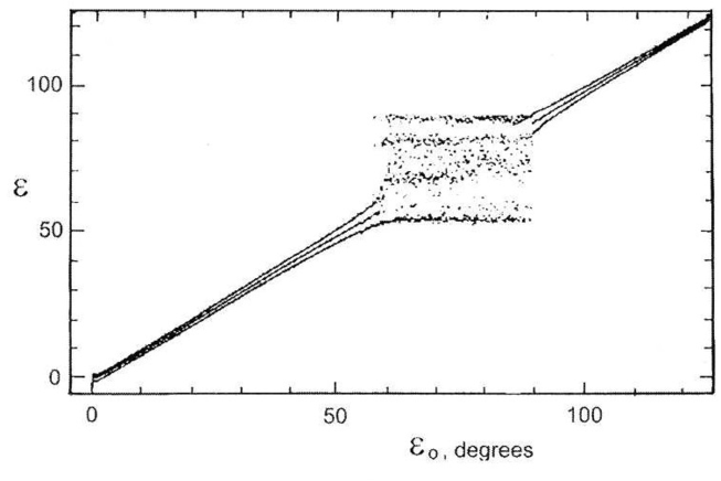
Figure 1: The maximum, mean and minimum obliquity variations of the Earth depending on the initial obliquity $\epsilon_{0}$. Note the chaotic zone at $\epsilon_{0}=60^{\circ}-90^{\circ}$ and the stability for its other values. The present obliquity of the Earth is within the stability zone due to the presence of the Moon, and transfers into the chaotic zone at the absence of the Moon (Laskar et al 1993).

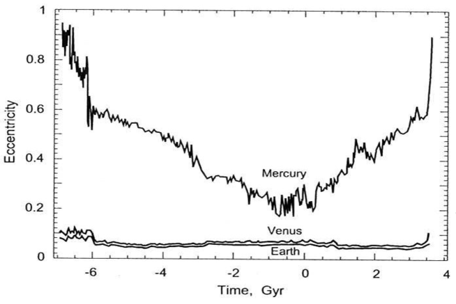
Figure 2: The variation of the eccentricities of Mercury, Venus and Earth by time. The chaotic variations are suppressed for the Earth and Venus, but are significant enough for Mercury, and will lead to its escape from the Solar system within a period less than 3.5 Gyr (Laskar 1994).

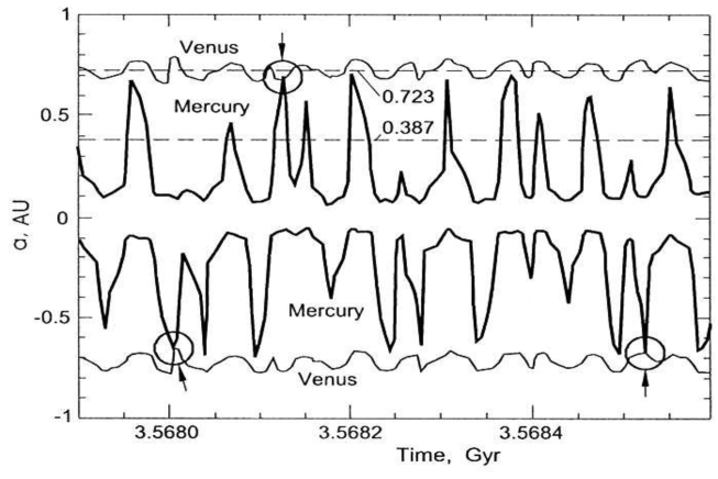
Figure 3: The overlapping of the major semi-axes of orbits of Mercury and Venus due to chaotic effects (Laskar 1994).

Numerical integration with a time step of 500 years over the time span of about 200 million years reveals that the inner planets of the Solar system are chaotic, due to the presence of two secular resonances, one due to Mars and Earth at $\theta=2(g_{4}-g_{3})-(s_{4}-s_{3})$ and another due to Mercury, Venus and Jupiter at $\sigma=(g_{1}-g_{5})-(s_{1}-s_{2})$, where $g_{i}$ and $s_{i}$ are the frequencies of the perihelions and nodes, respectively.

Laskar’s calculations revealed the chaotic behavior of Mercury’s orbit with eccentricity variations up to 0.05, which results in its overlapping with the orbit of Venus and with inevitable escape of Mercury from its orbit. Chaotic behavior was discovered also for the obliquities of the planets, particularly for Mars, varying from 0 to 60 degrees. Obviously, this fact has to be taken into account while studying the past evolution of the atmosphere of Mars. Chaotic behavior of the obliquity of the Earth would range even wider, within 0 and 85 degrees, with all dramatic consequences for the climate of the Earth, however, only at the absence of the Moon. The Moon therefore, is damping the obliquity variations up to 1.3 degrees, thus stabilizing the Earth’s climate[22].

We see that, the chaotic effects are not only able to influence essentially the dynamics of the Solar system but even the Earth’s climate.

4 Galactic Dynamics

4.1 N-body gravitating systems and geodesic flows

Many properties of statistical mechanics of globular clusters and galaxies can be studied considering a $N$-body gravitating system described by Hamiltonian

$$H(p,r) = \sum_{a=1}^{N}\sum_{i=1}^{3}\frac{p^{2}_{(a,i)}}{2m_{a}}+U(r),$$ (29)

$$U(r) = -\sum_{a<b}\frac{Gm_{a}m_{b}}{|r_{ab}|},$$ (31)

$$\quad r_{ab}=r_{a}-r_{b}.$$

We will use a well known method existing in classical mechanics, the Maupertuis principle[9], enabling one to represent a Hamiltonian system as a geodesic flow on some Riemannian manifold. In physical problems this approach was firstly used by Krylov[14] and in stellar dynamics in[24, 25].

By means of the Maupertuis principle the Hamiltonian equations

$$\dot{r}^{\mu}=\frac{\partial H}{\partial p_{\mu}},\qquad\dot{p}_{\mu}=-\frac{\partial H}{\partial r^{\mu}},$$ (32)

are reduced to the geodesic equation

$$\nabla_{u}u=0$$ (33)

on the region of configurational space

$$M=\{W=E-V(r)>0\}$$

with the Riemannian metric

$$ds^{2}=[E-V(r_{1,1},...,r_{N,3})]\sum_{a=1}^{N}\sum_{i=1}^{3}(dr_{a,i})^{2},$$ (34)

where $E$ is the total energy of the system. The condition of conservation of the total energy of the system

$$H(p,q)=E$$ (35)

is equivalent to the condition on the velocity associated with the geodesic

$$\parallel u\parallel=1,$$ (36)

while the affine parameter along the geodesic is determined by

$$ds=\sqrt{2}(E-V(r))dt.$$ (37)

The statistical properties of the geodesic flow are determined from the Jacobi equation

$$\nabla_{u}\nabla_{u}n+Riem(n,u)u=0.$$ (38)

For a vector field satisfying the orthogonality condition

$$<n,u>=0,$$ (39)

the Jacobi equation can be written in the form

$$\frac{d^{2}\parallel n\parallel^{2}}{ds^{2}}=-2K_{u,n}\parallel n\parallel^{2}+2\parallel\nabla_{u}n\parallel^{2},$$ (40)

where $K_{u,n}$ is the two-dimensional curvature

$$K_{u,n}=\frac{<Riem(n,u)u,n>}{\parallel u\parallel^{2}\parallel n\parallel^{2}-<u,n>^{2}}=\\ \frac{<Riem(n,u)u,n>}{\parallel n\parallel^{2}}.$$ (41)

Jacobi equation has the solution

$$\parallel n(s)\parallel\geq\frac{1}{2}\parallel n(0)\parallel\exp(\sqrt{-2k}s),\qquad s>0$$ (42)

if

$$k=\max_{u,n}\{K_{u,n}\}<0.$$ (43)

Then, the geodesic flow is an Anosov system.

Thus the negativity of the two-dimensional curvature the criterion of the instability of the geodesic flow.

4.2 Chaos of spherical systems

So, we have to calculate the two-dimensional curvature $K_{u,n}$ for the Hamiltonian ([ham]) for the gravitating N-body system. The Riemann curvature has the form[24, 25]

$$Riem_{\mu\lambda\nu\rho} = -\frac{1}{2W}[g_{\mu\nu}W_{\lambda\rho}+g_{\lambda\rho}W_{\mu\nu}-g_{\mu\rho}W_{\lambda\nu}-g_{\nu\rho}W_{\mu\lambda}]$$

$$-\frac{3}{4W^{2}}[(g_{\mu\lambda}W_{\nu}-g_{\mu\nu}W_{\lambda})W_{\rho}+(g_{\nu\rho}W_{\lambda}-g_{\lambda\rho}W_{\nu})W_{\mu}]$$

$$-\frac{1}{4W^{2}}[g_{\mu\nu}g_{\lambda\rho}-g_{\mu\lambda}g_{\nu\rho}]\parallel\partial W\parallel^{2},$$

where

$$g_{\mu\nu} = W\delta_{\mu\nu},$$

$$W_{\mu} = \frac{\partial W}{\partial r^{\mu}},\quad W_{\mu\nu}=\frac{\partial^{2}W}{\partial r^{\mu}\partial r^{\nu}}.$$

The analysis shows that $K_{u,n}$ is sign-indefinite, which means that no universal function

$$\tau:\hbox{(all $N$-body systems)}\to R_{+}$$

exists and hence no unique relaxation time scale can exist for all $N$-body gravitating systems.

For spherical systems,however, the two-dimensional curvature at large $N$ limit is shown to be strongly negative, since is determined by the scalar curvature $R$

$$K_{u,n}=\frac{R}{3N(3N-1)}$$ (44)

which is negative for $N>2$

$$R=-\frac{3N(3N-1)}{W^{3}}\left(\frac{1}{4}-\frac{1}{2N}\right)(\nabla W)^{2}-(3N-1)\frac{\Delta W}{W^{2}}<0.$$ (45)

Based on the mixing properties of dynamical systems described in previous sections, one can define the relaxation time for spherical systems. The explicit formula for that relaxation time taking into account the nonlinear interaction of all $N$ bodies of the system has been estimated in[24, 25] (see also[26]). For real stellar systems its value is shorter than the two-body relaxation time scale, but longer than the dynamical (crossing) time.

The disk gravitating systems can be studied using the Lie algebra of all vector fields with zero divergence on the two-dimensional torus $T^{2}$[27], since the kinetic energy of the element of the moving fluid induces a right–invariant Riemannian metric on $SDiff(T^{2})$. The principle of least action, which determines the motion of an incompressible fluid in terms of the geodesics of this metric, plays the role of the Maupertuis principle. One can show that, though the motion in disk galaxies is exponentially instable, the velocity field remains constant, so one cannot speak about a relaxation in the same sense as for spherical systems[28].

4.3 Relative chaos is stellar systems

The approach described above enables to consider instability of various configurations of stellar systems. Average the Jacobi equation over the geodesic deviation vector

$$\frac{d^{2}z}{ds^{2}}=\frac{1}{3N}r_{u}(s)+<\parallel\nabla_{u}n\parallel^{2}>,$$ (46)

where

$$n=z\hat{n},\qquad\parallel\hat{n}\parallel^{2}=1,$$

and $r_{u}(s)$ denotes the Ricci curvature in the direction of the velocity of the geodesic (Ric is the Ricci tensor)

$$r_{u}(s)=\frac{{\it Ric}(u,u)}{u^{2}}=\sum_{\mu=1}^{3N-1}K_{n_{\mu},u}(s),\qquad(n_{\mu}\bot n_{\nu},n_{\mu}\bot u).$$ (47)

The Ricci tensor has the expression

$$Ric_{\lambda\rho} = -\frac{1}{2W}[\Delta Wg_{\lambda\rho}+(3N-2)W_{\lambda\rho}]$$

$$+\frac{3}{4W^{2}}[(3N-2)W_{\lambda}W_{\rho}]-[\frac{3}{4W^{2}}-\frac{(3N-1)}{4W^{2}}]g_{\lambda\rho}\parallel dW\parallel^{2}.$$

Then the criterion of relative instability is[29]:

the more unstable of two systems is the one with smaller negative $r$

$$r=\frac{1}{3N}\inf_{0\leq s\leq s_{*}}[r_{u}(s)],\qquad r<0$$ (48)

within a given interval $0\leq s\leq s_{*}$, i.e., this system should be unstable with a higher probability in the same interval.

Numerical exploitation of the Ricci criterion of relative instability for the different models of stellar systems has shown that, e.g., a spherical system with a central mass is more unstable than a homogeneous one, spherical systems are more instable than disk-like ones, etc [29, 30, 31, 32].

5 Galaxy Clusters: Substructure and Bulk Flows

N-body gravitational systems, as we saw above, are exponentially instable systems. This fact gives a key to the possibility of reconstruction of certain properties of based on the limited observational information, which usually includes the 2D coordinates and 1D (line-of-sight) velocities and the magnitudes of the galaxies. We will show how one can reconstruct the hierarchical substructure and the bulk regular flows of the subgroups in the clusters of galaxies[7, 33].

The developed S-tree technique is based on the geometrical methods of theory of dynamical systems discussed in the previous sections, namely, on the introduction of the concept degree of boundness of N particles.

Consider two particles, so that $x_{1}(t)$ and $x_{2}(t),\ t\in(-T,T)$ are their trajectories when their interaction is taken into account, and $y_{1}(t)$ and $y_{2}(t)$, when the interaction is “switched off”.

It is easy to see that the deviation of trajectories within certain time interval

$$m=\max_{i=1,2}{\cal M}(x_{i}(\cdot)-y_{i}(\cdot)),$$ (49)

can be taken as a measure of the degree of boundness with respect to a local norm

$${\cal M}(x(\cdot))=\sup_{t\in(-T,T)}\{|x(t)|,|\dot{x}(t)|\}.$$ (50)

Consider balls of radius $r$ at each point of trajectories of the two interacting particles $x_{i}$. The union of those balls

$${\cal C}_{i}(r)=\bigcup_{t\in(-T,T)}B_{x_{i}(t)}(r),\ i=1,2\ .$$

of such minimal radius $m$ which contains all trajectories of the particles will denote the free corresponding particles.

Two particles are considered to be $\rho$-bound for $\rho>0$ if $m\leq\rho$.

This is easily generalized to any finite number of particles. $N$ particles labeled by the set of integers ${\cal A}=\{1,\ldots,N\}$ form a $\rho$-bound cluster if the distance between the corresponding trajectories of the system of interacting particles and free ones is less than the maximal deviation of all of the particles:

$$m=\max_{a\in{\cal A}}{\cal N}(x_{a}(\cdot)-y_{a}(\cdot))\leq\rho\ .$$ (51)

One can then define the boundness function so that for the given local norm ${\cal N}$

$${\cal P}_{Z}(Y)=\max_{a\in Y}{\cal N}(z_{a}(\cdot)-y_{a}(\cdot)),$$ (52)

where $z_{a}(t),y_{a}(t)$ are the solutions of the systems of equations I and II respectively for some time interval $(-T,T)$. In other words the boundness of ${\cal Y}$ in ${\cal Z}$ is the maximum deviation of the trajectories of its particles taking into account only internal interactions compared to the situation when interactions with particles in ${\cal Z}$ are also included. Our goal is to split ${\cal A}$ into $\rho$–subsystems, i.e., to obtain the map $\Sigma$ for this choice of boundness function.

The definition of a $\rho$–bound cluster given above can be reformulated now as a set of corresponding particles $A$ being a connected subgraph of the graph $\Gamma$ (equivalent the matrix) so that there is no other connected subgraph $B$ including $A:\ A\subset B.$ If one defines P as follows

$${\cal P}_{X}Y=\max\limits_{\stackrel{{\scriptstyle y\in Y}}{{z\in X\backslash Y}}}\{D_{yz}\}\ ,$$ (53)

the problem of the search of a $\rho$-bound cluster is reduced to that of a connected $\Gamma$-graph.

The algorithm of the construction of tree-diagram based on the estimation of the two-dimensional curvature as containing information both on the coordinates and velocities of the all particles, is developed and applied to various clusters of galaxies. As a result subgroups of galaxies, ”galaxy associations”, of specific dynamical properties, are detected in the studied Abell clusters[34], triggering later observations by the provided lists of galaxies (see, e.g.[36]). The S-tree method, together with certain general assumptions on the velocity distribution function of galaxies can be used for the determination of the bulk velocities of the subgroups.

Let us stress again, that these methods arise due to the nonlinearity of the N-body gravitating systems.

6 General Relativity and Cosmology

The impossibility of the direct application of results of theory of dynamical systems developed for Riemannian spaces is the main difficulty arising while studying the chaos in General Relativity and cosmology where one deals with pseudo-Riemannian spaces. Therefore, first, one has to reformulate the concepts described in previous sections and applied for astrophysical Newtonian systems, for the case of pseudo-Riemannian spaces. We will give the reformulation of the property of hyperbolicity and the covariant definition of the Lyapunov exponents given in[37], which are basic concepts for the study of chaos, and then, using it, will consider the stability of cosmological solutions, particularly, of inflationary ones.

I will not discuss the mixmaster models which had essentially provoked the studies on chaos in cosmology, since they are covered in Kirillov’s lectures at VIII Brazilian School of Cosmology and Gravitation[38]. For the further progress on those models in the context of Non-Abelian gauge, string theories and pre-Big-Bang scenarios I will refer to reviews[39, 40, 41].

6.1 Hyperbolicity in pseudo-Riemannian spaces

Consider a geodesic flow on $M$, i.e. a group of mappings $\{S^{t}\}$ of a space $T^{\lambda}M$

$$T^{\lambda}M=\{(x,u);x\in T_{x}M,g(u,u)=||u||^{2}=\lambda\},\,\lambda=0,\pm 1.$$

Each mapping performs a shift of a linear element $\xi=(x,u)$ along the geodesic on distance $t$.

Let $\gamma(t)$ be a geodesic on $M$ passing by a point $x\in M$, and $\{E_{a}\}$ is a fixed n-dimensional basis on $T_{x}M$.

Transferring $\{E_{a}\}$ parallel along $\gamma(t)$, i.e. getting a basis at every $t$, one has a Fermi basis on $T_{x}M$.

Each vector $X\in T_{\gamma}M$ can be represented via Fermi basis

$$X(t)=X^{a}(t)E_{a}.$$

with the E-norm

$$||X||^{2}_{E}=\Sigma(X_{a})^{2}$$

for basis $\{E_{a}\}$.

Let $\{E_{a^{\prime}}\}$ be another basis. Then a non-singular matrix $\Phi_{a}^{b^{\prime}}$ exists, such that

$$E_{a}=\Sigma\Phi_{a}^{b^{\prime}}E_{b^{\prime}}.$$

Since both $\{E_{a}\}$ and $\{E_{a^{\prime}}\}$ are Fermi bases, the latter relation has to be satisfied also for constant $\Phi_{a}^{b^{\prime}}$.

Then

$$X^{b^{\prime}}(t)=\Sigma\Phi_{a}^{b^{\prime}}X^{a}(t).$$

In view of non-singularity of $\Phi_{a}^{b^{\prime}}$, we can write

$$C\Sigma(X_{a})^{2}\leq\Sigma(X_{b^{\prime}})^{2}\leq C^{-1}\Sigma(X_{a})^{2}$$

or

$$C||X||_{E}^{2}\leq||X||_{E}^{2}\leq C^{-1}||X||_{E}^{2},$$

where $C$ is a positive constant.

Definition of hyperbolicity. Geodesic $\gamma_{x}(t)=S^{t}(\xi),||\dot{\gamma}_{x}(t)||^{2}=\lambda$ is $\lambda$-hyperbolic, if there exist subspaces $W^{s}(S^{t}(\xi))$ and $W^{u}(S^{t}(\xi))$ and $W^{0}(S^{t}(\xi))$ of the tangent space $T_{S^{t}(\xi)}T^{\lambda}M$ and numbers $A0,0<\mu<1$, such that

$$T_{S^{t}(\xi)}T^{\lambda}M=W^{s}(S^{t}(\xi))W^{u}(S^{t}(\xi))W^{0}(S^{t}(\xi)),$$

$$dS^{\tau}W^{s}(S^{t}(\xi))=W^{s}(S^{t+\tau}(\xi)),dS^{\tau}W^{u}(S^{t}(\xi))=W^{u}(S^{t}(\xi)),$$

where $W^{0}(S^{t}(\xi))$ is a 1D space defined by the flow vector.

For each $t,\tau>0$ and for a certain basis $\{E_{a}\}$ we have

$$||dS^{\tau}v||^{2}_{E}\leq A^{2}\mu^{2\tau}||v||^{2}_{E},v\in W^{s}(S^{t}(\xi)),$$

$$||dS^{\tau}v||^{2}_{E}\geq A^{-2}\mu^{-2\tau}||v||^{2}_{E},v\in W^{u}(S^{t}(\xi)),$$

where

$$||v||^{2}_{E}=||d\pi_{\lambda}v||^{2}_{E}+||Kv||^{2}_{E},v\in TT^{\lambda}M,\pi_{\lambda}:TT^{\lambda}M\rightarrow TM,$$

and $K$ is the mapping of connection $\nabla$.

The definition is $\{E_{a}\}$ invariant.

Definition Geodesic flow is $\lambda-$hyperbolic if its all geodesics are $\lambda$-hyperbolic.

Jacobi field is defined along the geodesic determined by the Jacobi equation

$$\nabla_{u}\nabla_{u}Y+R(u,v)Y=0.$$

Correspond now to each vector $v\in TT^{\lambda}M$ a solution $Y(t)$ of Jacobi equation with initial conditions

$$Y_{v}(0)=d\pi v,\nabla_{u}Y_{v}(0)=kv.$$

The resulting mapping

$$f:v\rightarrow Y_{v}(t)$$

is an isomorphism and

$$d\pi dS^{t}(v)=Y_{v}(t),KdS^{t}v=\nabla_{v}Y_{v}(t).$$

From the Jacobi equation we have

$$||dS^{t}v||^{2}_{E}=||Y_{v}(t)||^{2}_{E}+||\nabla_{u}Y_{u}(t)||^{2}_{E}.$$

the latter equation and the Jacobi one enable to check the hyperbolicity condition.

Definition. Lyapunov characteristic exponent for maximal geodesic $\gamma$ and vector $v$ is defined as

$$\chi(\gamma,v)=\lim_{t\rightarrow\infty}\sup\frac{ln||dS^{t}_{\dot{\gamma}}v||^{2}_{E}}{2t}.$$

Definition. Geodesic $\gamma$ is stable if for any $\epsilon>0,\exists\delta(\epsilon>0$ such that from $||v||^{2}_{E}<\delta$ follows the condition $||dS^{t}_{\dot{\gamma}}v||^{2}<\epsilon$ for any $t$. Otherwise $\gamma$ is unstable. The latter two definitions are also basis-invariant.

Let us now define a convenient basis.

For arbitrary geodesic $\gamma(t)$ we choose the following orthonormal basis at point $\gamma(t)$

$$E_{0}=\gamma(0)=u,E_{1},...,E_{n-1};$$

$$g(E_{a},E_{b})=$$

where $E_{a}$ is a dual basis.

If the following conditions are satisfied

$$\nabla_{u}E_{a}=0=\nabla_{u}E^{b},$$

then the basis on $T^{0}M$ can be defined as

$$E_{0}=u,g(E_{a},E_{b})=$$

and on $T^{1}M$

$$E_{0}=u,g(E_{a},E_{b})=$$

For the vector field

$$Y(t)=Z^{a}(t)E_{a}$$

the Jacobi equation can be written in the form

$$Z^{a}(t)+K^{a}_{b}(t)Z^{b}(t)=0,$$

where

$$K^{a}_{b}=<E^{a},R(u,E{-b})u>=R^{a}_{bcd}u^{c}u^{d}.$$

For the above defined basis on $T^{0}M$ and the Jacobi equation we have

$$\dot{Z}=1.$$

which means that none of geodesic flows can be 0-hyperbolic.

It can be shown that the definitions given above for spaces of Lorentzian signature (-,+,…,+), can be generalized for the signatures (-, ,-, +, ,+).

The covariant definition of hyperbolicity and Lyapunov exponents given above enable the consideration of the stability problem of cosmological solutions.

6.2 The ADM principle and geodesic flows in Wheeler-DeWitt superspace

The problem of the stability of cosmological solutions is a problem of stability in Wheeler-DeWitt superspace. We will consider this problem using the method of geodesic flows[42]. So, first, we have to define the Hamiltonian system, then reduce it to a flow of geodesics using the definition of the hyperbolicity given in the previous section.

Arnowitt-Deser-Misner (ADM) method provides the scheme of the sought Hamiltonian formulation, assuming as given the 3-geometries of the initial and final Cauchy hypersurfaces. We will consider locally isotropic and homogeneous cosmological models with scalar field when the metric can be given as

$$h_{ij}=\sigma^{2}\bar{h}_{ij}$$

where

$$\sigma^{2}=\frac{4\pi G}{3}[\int\bar{h}^{1/2}d^{3}x]^{-1},\,\bar{h}=det\bar{h}_{ij}$$

We consider the Lagrangian of the scalar field

$$L_{\phi}=-g^{-1/2}[\phi_{,a}\phi_{,b}g^{ab}+V(\phi)]$$

and the action

$$I=\int p_{\alpha}d\alpha+p_{\chi}d\chi-N\rm{H}_{ADM}dt$$

where the ADM Hamiltonian is

$$\rm{H}_{ADM}=\frac{1}{2}e^{-3\alpha}[-p^{2}_{\alpha}+p^{2}_{\chi}]+e^{3\alpha}[U(x)-\frac{k}{2}e^{-2\alpha}],$$

where

$$\alpha=lna,\,\chi=\sigma\phi,U(x)=\frac{4\pi G\sigma^{2}}{3}V(\phi).$$

As usual variation with respect the lapse function $N$ leads to the condition

$$\rm{H}_{ADM}=0.$$

To reduce the Hamiltonian system to the geodesic flow let us split the hypersurface into the following regions

$$W^{+}\{x|V(x)>0\},\,W^{-}\{x|V(x)<0\},$$

so that if the metric in region $W^{-}$ is Riemannian, then

$$g_{ab}v^{a}v^{b}=-2V>0,d\tau=(g_{ab}u^{a}u^{b}/-2V)^{-1/2}ds$$

and we can write the variation

$$extI|_{H=0}=ext\int(-2V)^{1/2}(g_{ab}u^{a}u^{b})^{1/2}ds=ext\int(G_{ab}u^{a}u^{b})^{1/2}ds.$$

Here $G_{ab}=-Vg_{ab}$ is also a Riemannian metric.

Choosing the affine parameter $s$ in order to satisfy the condition

$$||u||^{2}=G_{ab}u^{a}u^{b}=1$$

we have

$$G_{ab}u^{a}u^{b}=-Vg_{ab}v^{a}v^{b}(d\tau/ds)^{2}=2V^{2}(d\tau/ds)^{2}.$$

Reparameterizing the affine parameter

$$ds=2^{1/2}(-V)d\tau,$$

we arrive at the flow of geodesics in the region $W^{-}$

$$\rm{H}=1/2g^{ab}p_{a}p_{b}+V\rightarrow\{G_{ab}=-Vg_{ab},\,ds=2^{1/2}(-V)d\tau,||u||^{2}=1\}.$$

As regards for the region $W^{+}$, the classical system cannot end up in it.

Now, if the metric $g$ is pseudo-Riemannian, following the same scheme we end up with the geodesic flow

$$\rm{H}\rightarrow\{|V|g_{ab},\,2^{1/2}|V|d\tau,-signV\}.$$

Thus, we reduced the ADM Hamiltonian system to a geodesic flow on a pseudo-Riemannian manifold.

To study the stability of the geodesic flow we have to proceed from the Jacobi equation, which has the form

$$\frac{d^{2}z^{i}}{d\tau^{2}}+\gamma(z)\frac{dz^{i}}{d\tau}+\omega^{i}_{j}(z)=0,$$

where

$$\gamma=-\frac{d}{d\tau}ln|V|,\omega^{i}_{j}=2V^{2}K_{j}^{i},i,j,=1,2...k-1.$$

Using the variables

$$z^{i}=AY^{i}$$

we arrive to the equation

$$\dot{Y}^{i}+2(\dot{A}/A+\gamma)\dot{Y}^{i}+[(\dot{A}/A+\gamma\dot{A}/A))\delta_{j}^{i}+\omega^{i}_{j}]Y^{j}=0$$

where

$$\dot{A}/A=-1/2\gamma,A=|V|^{1/2}.$$

Particularly for the case $k=0$ we have the simplified expressions

$$G=e^{6\alpha}|U|,|V|=e^{3\alpha}|U|,$$

$$\gamma(\tau)=-3\frac{d\alpha}{d\tau}-\frac{1}{U}\frac{dU}{d\tau}$$

$$K(\tau)=-\frac{1}{2}\frac{DlnG}{G}=-\frac{1}{2}\frac{lnD|V|}{e^{6\alpha}|U|},$$

$$\omega(\tau)=UDln|U|,D=-\frac{\partial^{2}}{\partial\alpha^{2}}+\frac{\partial^{2}}{\partial\chi^{2}}.$$

6.3 Stability of inflationary solutions

Consider the scalar field

$$U=\lambda\chi^{n}/n$$

and the conditions

$$\dot{H}<<H^{2},\dot{\chi}^{2}<<U,|\dot{\chi}/\chi|<<H$$

and $\chi>>1$ at $\alpha\rightarrow\infty$. Then we have

$$\dot{\gamma}=-3\dot{H},\frac{1}{2}\dot{\gamma}+\frac{\gamma^{2}}{4}\simeq\frac{9}{4}H^{2},$$

and the Jacobi equation

$$\dot{Y}^{i}-[-\frac{nU}{\chi^{2}}+(\frac{3}{2}H)^{2}]Y=0.$$

From the Einstein equation

$$\dot{H}+3H^{2}=6U,$$

and in view of the condition $\dot{H}<<H^{2}$ we have $H^{2}\simeq 2U$. If $\chi>>(2n/3)^{1/2}$, then $nU/\chi^{2}<<9/4H^{2}$, and we have the Jacobi equation in a simple form

$$\dot{Y}-(9/4\dot{\alpha}^{2})Y=0.$$

From its solution we obtain

$$\delta^{2}=z^{2}+\dot{z}^{2}\simeq const\,U+const\,\frac{U^{{}^{\prime}4}}{U^{2}}\simeq const\,\chi^{n}+const\,\chi^{2n-4}.$$

We see that $\delta$ decreases for any $n>2$ and therefore we have Lyapunov stability of the inflationary solutions. The last formula enables also to obtain the law of the decay of perturbations at various $n$. For example at $n=4$ we have exponential decay of perturbations, and the larger is $n$, the more stable the solution is.

Thus we showed how one can deal with the stability problem in pseudo-Riemannian spaces, and illustrated this on inflationary solutions.

7 Instability in Superspace

How typical is the given cosmological solution? This is a basic question posed since the early days of the study of the Einstein equations. In the context of later developments, particularly in quantum cosmology, the question can be reformulated in the form: to what degree are the minisuperspace models typical in superspace given the huge extrapolations involved? The consideration of perturbed minisuperspace models by Hawking and other authors still involves extrapolation in the absence of a deeper merging of quantum theory and gravity.

The study of dynamics in the Wheeler-DeWitt superspace, more precisely, the properties of geodesic flows in superspace can provide a more general view of how typical the minisuperspace models are. The problem, however, is far more difficult than the one posed in conventional hyperbolicity theory, since one deals both with infinite dimensional and pseudo-Riemannian manifolds.

However, hyperbolicity can be defined for such manifolds and we will consider the case of homogeneous cosmological models [43].

The metric of Wheeler-DeWitt superspace is

$$G^{ijkl}=\frac{1}{2}[\gamma^{ik}\gamma^{jl}+\gamma^{il}\gamma^{jk}-2\gamma^{ij}\gamma^{kl}],$$

where

$$\gamma=det\gamma_{ij},i,j,k,l=1,...,n.$$

Then one can derive

$$G^{ijkl}d\gamma_{ij}d\gamma_{jl}=-d\xi^{2}+\frac{n\xi^{2}}{16(n-1)}tr(\gamma^{-1}\partial\gamma/\partial\xi^{A}\gamma^{-1}\partial\gamma/\partial\xi^{B})\,d\xi^{A}d\xi^{B}\,$$

where

$$\xi=4((n-1)/n)^{1/2}\gamma^{1/4}\,,\ A,B=1,...,n(n+1)/2-1\,,$$

Then, moving to the subspace of superspace

$$\bar{W}=(\gamma_{ij};\gamma_{ij}\in W,\gamma=1)$$

with a metric induced by the metric of the superspace $W$

$$G_{AB}d\xi^{A}d\xi^{B}=tr(\gamma^{-1}\partial\gamma/\partial\xi^{A}\gamma^{-1}\partial\gamma/\partial\xi^{B})\,d\xi^{A}d\xi^{B}\,,$$

the existence of non-zero Lyapunov numbers

$$\Sigma_{i}\omega_{i}=-n/4<0\,$$

can be shown for the solutions of the Jacobi equation

$$z^{a}_{i}(t)=x^{a}_{i}\exp[(\pm(-\omega_{i})^{1/2}t]\,.$$

This implies the exponential instability of the geodesic flow in that subspace of the superspace.

For models with a scalar field Armen Kocharyan[44] was able to show that the instability is exponential if:

1. Gravitational and matter fields vary quickly with respect the potential;

2. The Universe undergoes inflation in a local domain.

The smaller are the dimension and the number of scalar fields, the stronger is the instability.

These results lead to the following general conclusion:

The quantized system in a finite-dimensional submanifold is not typical to that in superspace due to the existence of virtual perturbations along the frozen directions which are unstable.

This implies that minisuperspace models cannot be considered as fair approximations of superspace models.

8 Conclusion

I stop here. As we saw, chaos is an inevitable ingredient of the Universe, but it needs particular efforts to deal with.

The spectrum of the methods applied will obviously grow further. I conclude with mentioning the use of Kolmogorov complexity (algorithmic information) for the study of properties of Cosmic Background Radiation and relations of the latter with thermodynamical and cosmological arrows.[45, 46, 47]

References

- [1] Sagdeev R.Z., Usikov D.A., Zaslavsky G.M., Nonlinear Physics, Harwood, 1988.
- [2] Lichtenberg A.J., Lieberman M.A., Regular and Chaotic Dynamics, Springer, 1992.
- [3] Ott E., Chaos in Dynamical Systems, Cambridge University Press, 1993.
- [4] Zaslavsky G.M., Physics of Chaos in Hamiltonian Dynamics, Imperial College Press, 1998.
- [5] Gurzadyan V.G., Pffeniger D. (Eds.), Ergodic Concepts in Stellar Dynamics, Springer. 1994.
- [6] Hobill D., Burd A., Coley A. (Eds.), Deterministic Chaos in General Relativity, Plenum, 1994.
- [7] Gurzadyan V.G., Kocharyan A.A., Paradigms of the Large-Scale Universe, Gordon and Breach, 1994.
- [8] Gurzadyan V.G., Ruffini R. (Eds.), The Chaotic Universe, World Scientific, 2000.
- [9] Arnold V.I., Mathematical Methods of Classical Mechanics, Springer, 1989.
- [10] Dynamical Systems. Modern Problems in Mathematics, vols.1,2, Ed.Ya.G.Sinai, Springer, 1989.
- [11] Katok A., Hassenblatt B., Introduction to the Modern Theory of Dynamical Systems, Cambridge University Press, 1996.
- [12] Smale S., Finding a Horseshoe on the Beaces of Rio, in: The Chaos Avant-Garde: Memories of the Early Days of Chaos Theory, World Scientific, 2000.
- [13] Anosov D.V., Geodesic Flows on Closed Riemannian Spaces with Negative Curvature, Comm. MIAN, vol.90, 1967.
- [14] Krylov N.S., Studies on Foundation of Statistical Mechanics, Publ. AN SSSR, Leningrad, 1950.
- [15] Pfenniger D., A&A,165, 74, 1986.
- [16] Murray C.D., Dermott S.F., Solar System Dynamics, Cambridge University Press, 1999.
- [17] Lecar M. et al, Ann.Rev.Astron.Astroph. 39, 581, 2001.
- [18] Morbidelli A., Modern Celestial Mechanics, Taylor and Francis, 2002.
- [19] Kolmogorov A.N., Doklady AN SSSR, 98, 527, 1954.
- [20] Laskar J., Physica D, 67, 257, 1993.
- [21] Laskar J. Robutel P., Nature, 361, 608, 1993.
- [22] Laskar J. Joutel F., Robutel P., Nature, 361, 615, 1993.
- [23] Laskar J., A&A, 287, L9, 1994.
- [24] Gurzadyan V.G., Savvidy G.K., Doklady AN SSSR, 277, 69, 1984.
- [25] Gurzadyan V.G., Savvidy G.K., A&A, 160, 203, 1986.
- [26] Lang K.R., Astrophysical Formulae, vol.II,p.95, Springer, 1999.
- [27] Arnold V.I., Annales de l’Institute Fourier, XVI, 319, 1966.
- [28] Gurzadyan V.G., Kocharyan A.A., A&A, 205, 93, 1988.
- [29] Gurzadyan V.G., Kocharyan A.A., Ap&SS, 135, 307, 1987.
- [30] El-Zant A.A., A&A, 326, 113, 1997.
- [31] El-Zant A.A., Gurzadyan V.G., Physica D, 122, 241, 1998.
- [32] Bekarian K.M., Melkonian A.A., Astronomy Lett., 11, 323, 2000.
- [33] Bekarian K.M., Melkonian A.A., Complex Systems, 11, 323, 1997.
- [34] Gurzadyan V.G., Mazure A., MNRAS, 295, 177, 1998.
- [35] Bekarian K.M., Ph.D Thesis, Yerevan State University, 2001.
- [36] Mario-Franch A., Aparicio A., ApJ, 568, 174, 2002.
- [37] Gurzadyan V.G., Kocharyan A.A., YerPhI-920(71), Yerevan Physics Institute, 1986.
- [38] Kirillov A.A., in: Cosmology and Gravitation, Ed.M.Novello, Editions Frontieres, 1996.
- [39] Belinski V. in[8]
- [40] Matinyan S.G., in: Proc.IX Marcel Grossmann meeting, World Scientific, 2002; gr-qc/0010054.
- [41] Damour T., hep-th/0204017, 2002.
- [42] Gurzadyan V.G., Kocharyan A.A., Sov.Phys-JETP, 66, 651, 1988.
- [43] Gurzadyan V.G., Kocharyan A.A., Mod.Phys.Lett. 2A, 921. 1988.
- [44] Kocharyan A.A., Comm.Math.Physics, 143, 27, 1991.
- [45] Gurzadyan V.G., Europhys.Lett. 46, 114, 1999.
- [46] Gurzadyan V.G., Ade P.A.R., de Bernardis P., Bianco C.L., Bock J.J., Boscaleri A., Crill B.P., De Troia G., Ganga K., Giacometti M., Hivon E., Hristov V.V., Kashin A.L., Lange A.E., Masi S., Mauskopf P.D., Montroy T., Natoli P., Netterfield C.B., Pascale E., Piacentini F., Polenta G., Ruhl J., astro-ph/0210021, 2002.
- [47] Allahverdyan A.E., Gurzadyan V.G. J.Phys.A, 35, 7243, 2002.