The lens and source of the optical Einstein ring gravitational lens ER 0047–2808

Abstract

We perform a detailed analysis of the optical gravitational lens ER 0047–2808 imaged with WFPC2 on the Hubble Space Telescope. Using software specifically designed for the analysis of resolved gravitational lens systems, we focus on how the image alone can constrain the mass distribution in the lens galaxy. We find the data are of sufficient quality to strongly constrain the lens model with no a priori assumptions about the source. Using a variety of mass models, we find statistically acceptable results for elliptical isothermal-like models with an Einstein radius of 1.17^′′. An elliptical power-law model ($\Sigma\propto R^{-\beta}$) for the surface mass density favours a slope slightly steeper than isothermal with $\beta=1.08\pm 0.03$. Other models including a constant M/L, pure NFW halo and (surprisingly) an isothermal sphere with external shear are ruled out by the data. We find the galaxy light profile can only be fit with a Sérsic plus point source model. The resulting total M/L_B contained within the images is $4.7h_{65}\pm 0.3$. In addition, we find the luminous matter is aligned with the total mass distribution within a few degrees. This is the first time a resolved optical gravitational lens image has been quantitatively reproduced using a non-parametric source.

The source, reconstructed by the software, is revealed to have two bright regions, with an unresolved component inside the caustic and a resolved component straddling a fold caustic. The angular size of the entire source is $\sim 0.1$^′′and its (unlensed) Lyman-$\alpha$ flux is $3\times 10^{-17}$ erg s^-1 cm^-2.

1 Introduction

The discovery (Hewitt et al. 1988; Langston et al. 1989) and subsequent modelling (Kochanek & Narayan 1992a; Kochanek 1995) of Einstein ring gravitational lenses at radio wavelengths raised the prospect of obtaining detailed quantitative information for both the lensed sources and the form of the mass distribution in the intervening lensing galaxies. Kochanek (1995) compared mass models for the lensed radio lobe MG1654+134 using LensCLEAN (Kochanek & Narayan 1992b) in image space. It was subsequently shown that LensCLEAN-ing radio data in image space can introduce biases, hence visibility-based LensCLEAN was introduced (Ellithorpe et al. 1996; Wucknitz 2004). Wucknitz et al. (2004) recently used this method to measure $H_{0}$ in B0218+357.

Recent work at optical/near-IR wavelengths (Kochanek et al. 2000, 2001) has concentrated on what can be learnt using infrared images of Einstein rings. Miralda-Escude & Lehar (1992) pointed out that there should exist a much larger number of Einstein rings detectable at optical wavelengths, and systematic surveys for such systems are now underway (Hewett et al. 2000). ER 0047–2808, the first known example of a galaxy lensing another normal galaxy, was the first Einstein ring to be discovered at optical wavelengths (Warren et al. 1996). The ER 0047–2808 system, together with the recently discovered lens 1RXS J113155.4-123155 (Sluse et al. 2003), are the only Einstein ring systems with good S/N Hubble Space Telescope (HST) images at optical wavelengths. Modelling of the system, exploiting the extended surface brightness distribution of the lensed source, would provide details of the source morphology and allow some discrimination between models for the mass distribution in the intervening lensing galaxy. Compilation of a large sample of optical Einstein rings could provide information on the luminosity function and morphologies of star–forming galaxies at redshifts $z=3-5$ whose (unlensed) magnitudes remain too faint for direct study using even 8m–class telescopes. Similarly, statistical properties derived from a large sample of such lensed systems, will provide new information on the still poorly constrained distribution of mass in massive early–type galaxies, which form the majority of the deflector population.

As a first step toward achieving these goals, this paper presents an analysis of the HST imaging observations of ER 0047–2808. This system has been studied by Koopmans & Treu (2003, hereafter ‘KT03’), who combined dynamical information (the stellar velocity dispersion profile), with gravitational lens information (the angular size of the Einstein ring), to draw conclusions on the mass profiles of both the visible and dark matter. The HST image was used simply to determine the total mass within the ring, and to measure the lens galaxy light profile. In our complementary analysis, we concentrate on extracting as much information on the mass profile as possible from the image alone. We use software based on the LensMEM method (Wallington et al. 1996, hereafter ‘WKN96’) to perform a gravitational–lens inversion of the complete surface brightness distribution around the ring. This allows us to draw conclusions on the radial distribution of the (total) mass, and also produces new insight into the source morphology. An advantage of the optical CCD image over radio images is that the counts in the pixels are independent, so that an unambiguous goodness–of–fit statistic may be measured. To analyse a radio image properly requires the covariance matrix for the image pixels, or to work directly with the visibilities (Ellithorpe et al. 1996; Wucknitz 2004).

Section 2 describes the HST WFPC2 observations, the data reduction steps, the determination of the noise characteristics of the final image of ER 0047–2808, and the accurate measurement of the surface brightness profile of the lensing galaxy. Section 3 presents details of the lens modelling algorithm. Seven different mass models for the lens are considered. Four of the mass models provide satisfactory fits to the data, whereas three are rejected. A discussion of the results, and comparison with the analysis of KT03, is given in Section 4, before the principal conclusions are summarised in the final section.

Throughout this paper, we assume a $\Lambda$CDM cosmology with $\Omega_{\Lambda}=0.7$, $\Omega_{m}=0.3$ and $H_{0}=65\ {\rm km\,s^{-1}\,Mpc^{-1}}$ (for consistency with KT03) unless otherwise stated.

2 Observations and data reduction

2.1 Observations and frame combination

ER 0047–2808 was observed with the WFPC2 instrument on HST over four orbits, on 1999 January 7. The target was placed on chip 4 (pixel size 0.1″) of the WFPC2 and exposures were made using the F555W filter, which contains the strong Ly$\alpha$ emission line, at $z=3.67$, of the lensed source. A dither step was applied between orbits, on a $2\times 2$ grid with step size $N+0.5$ pixels, in order to improve the sampling. Two equal exposures of $1200\,$s were made per orbit, with the exception that the first exposure of the first orbit was only $1100\,$s due to the field acquisition overhead. The data were processed through the WFPC2 pipeline using the latest calibration frames.

The first step in combining the frames was to subtract the average counts in the background from each frame. We then used the dither software (Fruchter & Hook 2002) to identify and eliminate cosmic rays and then to interlace the data into the half–pixel grid. In dither parlance, interlacing corresponds to using a delta–function drizzle footprint, pixfrac=0.0. This was done to ensure that the data in each pixel remain independent. For the same reason we did not apply the distortion–coefficient corrections to linearise the astrometry of the field. The lack of accurate astrometry over the field is not a concern since we are only interested in the immediate vicinity of the lensing galaxy.

Cosmic–rays pose a problem since there are only two exposures per pixel. To identify cosmic–rays we firstly drizzled the data using a fat footprint, pixfrac=1.0, to form a slightly smoothed combined image. In this way information from adjacent pixels contributes to the estimate of the counts in a particular interlaced pixel. The combined image can then be used to identify where the counts in any individual exposure are abnormally high. Specifically, the routine driz_cr compares the drizzled image against the eight individual exposures to identify cosmic rays in each exposure. The affected pixels were then masked, an improved average frame was formed, and further cosmic–rays were identified. In the region around the galaxy we checked carefully the cosmic–ray identifications of driz_cr in order to ensure the $\sigma$–rejection level was set at a value close to optimal. The driz_cr routine proved to be highly effective. Once the cosmic–ray masks for the eight individual exposures had been defined the data were interlaced, averaging the data pairs, after scaling all frames to a common exposure time of $1187.5\,$s.

The final combined frame is shown in Fig. 1 (LHS). The pixels are shown with side 0.05″, i.e. half the original pixel size, since this is the interlaced pixel separation. However, it should be understood that this is for illustration only. Since the data have been interlaced, the original pixel size, i.e. 0.1″, has been retained. In other words, Fig. 1 illustrates four frames simultaneously, each offset from each other on a $2\times 2$ grid of side 0.05″. In all the fits described in this paper we account for this data format. This is necessary because of the undersampling of the WFPC2 point spread function (PSF).

The image contains a large number of useful pixels for measuring the surface brightness distribution of the lens galaxy ($\sim 10^{4}$) and the Einstein ring ($\sim 10^{3}$). In such cases it is essential to establish the accuracy to which the uncertainty of the counts in each pixel is known. This is because the corresponding uncertainty to which $\chi^{2}$ may be determined can be as large, or larger, than the width of the $\chi^{2}$ distribution itself. For example, if the number of degrees of freedom in the model fitting ($\simeq$ no. pixels) is $\sim 10^{4}$, the reduced $\chi^{2}$ is normally distributed as $\chi^{2}_{\nu}=1.0\pm\sqrt{2/\nu}=1.0\pm 0.014$. For this case, in order that the uncertainty in $\chi^{2}$ is not dominated by the uncertainty in the determination of the noise in each pixel, it would be necessary to determine the noise to a fractional accuracy substantially better than $0.007$.

A Poisson estimate of the $1\sigma$ noise–frame was computed, incorporating read and photon noise, and accounting for elimination of data due to cosmic–rays, i.e. whether 0, 1, or 2 exposures contribute to an individual pixel. Standard WFPC2 values of the read–noise, $5e^{-}$, and gain, $7e^{-}/ADU$, were adopted. To check the accuracy of the estimated uncertainties, the final combined data frame was divided by the $1\sigma$ noise–frame to form a signal–to–noise ratio (S/N) frame. The standard deviation of the counts in the background, which should be unity if the uncertainties are correct, was found to be $1.06\pm 0.01$, where the quoted uncertainty in this value was established from the scatter in measurements from several areas around the frame. It is unclear whether the small underestimate of the noise is due to lack of precision in the value of the read noise or the value of the gain. Therefore, the $1\sigma$ noise–frame was simply scaled by a factor $1.06$. The accuracy with which this scaling can be measured, $1\%$, means that the uncertainty in measured values of $\chi^{2}$ is $2\%$.

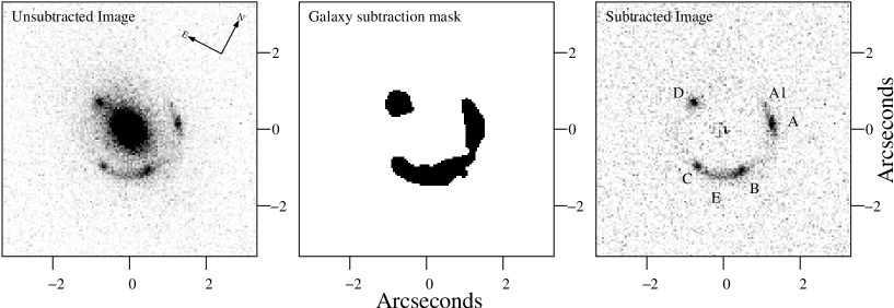
Figure 1: The figure shows a region $6.55\arcsec\times 6.55\arcsec$ ($131\times 131$ pixels) centred on the lens galaxy of ER 0047–2808; LHS: the interlaced final WFPC2 image, centre: the mask used in the galaxy fit, RHS: after subtraction of the galaxy image (as described in the text). The four bright spots in the image are labelled A–D. The arc of extended emission between B & C is labelled E. The small arc of extended emission north–east of A is labelled A1

2.2 Galaxy surface brightness profile

To subtract the image of the galaxy, necessary to isolate the image of the lensed source, we fitted parameterised 2–D models of the galaxy surface brightness profile convolved with the point spread function, using a modification of our own software (Warren et al. 2001) appropriate for drizzled data. The goodness–of–fit was calculated by summing $\chi^{2}$ over the four separate interlaced frames. To prevent the presence of the lensed background source from affecting the model fit to the galaxy, we masked out pixels in the vicinity of the Einstein ring. This was achieved in an iterative fashion, firstly subtracting the galaxy fit, then smoothing and thresholding the residuals to create a first mask, then refitting, and then refining the mask, etc. The final mask contains 842 pixels and is shown in Fig. 1 (centre).

Fitting the surface brightness profiles of early–type galaxies, which are cuspy at the centre, requires care, particularly where the data are undersampled. To generate a model image for each interlaced frame, the model galaxy profile was firstly integrated over sub–pixels of size $0.1\arcsec/3$. The PSF was computed using the tinytim software (Krist 1993, 1995), integrated over the same sub–pixel size. The model image was then convolved with the model PSF. The HST PSF is undersampled by WFPC2 at the wavelength of our observations and the sub–pixelation is necessary to correctly reproduce the actual image that would be seen by the detector. After rebinning this convolved image to the full $0.1\arcsec$ pixel size, the image was further convolved with the WFPC2 pixel scattering function, as the final step in forming a model image. The pixel scattering function accounts for the diffusion of electrons from the collecting pixel into nearby pixels. We used the $3\times 3$ kernel specified in the WFPC2 Instrument Handbook (Biretta et al. 2002). For this kernel, a fraction 0.365 of the collected electrons diffuse out of the central pixel, principally into the four nearest pixels. So the scattering function broadens the PSF significantly. Because of the cuspy galaxy light profile, the kernel is an essential element in the model fitting. However, the kernel was determined from pre–flight measurements, and it has not been remeasured in orbit. Therefore, somewhat surprisingly, it is a significant source of uncertainty (see below).

In the following we use $X,Y$ for the coordinates on the CCD, and $x,y$ for, respectively, the major and minor principal axes of any ellipse. The radius $R$ is defined by $R^{2}=x^{2}q+y^{2}/q$, where $q=b/a$ is the ellipse axis ratio. The galaxy model parameters are the $X,Y$ position of the centre, the axis ratio $q$, and the angle of orientation $\phi$, plus the parameters of the function defining the surface brightness profile. A de Vaucouleurs profile (de Vaucouleurs 1948) did not provide a satisfactory fit, so a Sérsic model (Sérsic 1968), where the surface brightness as a function of $R$ is $S(R)=S_{1/2}\exp\{-B(n)[(R/R_{1/2})^{1/n}-1]\}$, was tried. The parameter $n$ quantifies the shape of the profile: the values $n=0.5$, $n=1$, and $n=4$ correspond to the Gaussian, exponential, and de Vaucouleurs profiles. Profiles with larger $n$ are more sharply peaked. For cuspy galaxies, $n>3$, special care is needed in integrating the Sérsic function over sub–pixels near the centre. $B(n)$ is a constant for particular $n$, and we used the series asymptotic solution for $B(n)$ provided by Ciotti & Bertin (1999).

With the Sérsic function we obtained fits that were globally satisfactory, in terms of $\chi^{2}$. Nevertheless the fit over the central $0.5\times 0.5\arcsec$ was bad. We also found that the fitted value of $n$ depended sensitively on the size of the box, increasing as the box size diminished. This could be because either the Sérsic profile is not cuspy enough for this galaxy, or the pixel scattering kernel used is too broad. To investigate the latter we modified the kernel, reducing the scattered fraction from 0.365 to 0.2, but the central fit was still unsatisfactory. We therefore retained the standard kernel, and added a point source at the centre of the model surface brightness profile. The full model has 8 free parameters; $X,Y,q,\phi,S_{1/2},R_{1/2},n$, and $p$, the counts in the point source. Here it should be understood that $R_{1/2}$ is the half–light radius of the Sérsic component of the light profile, and not the radius containing half the total galaxy light. The final fit was made to a square–region, $131\times 131$ drizzled pixels, i.e. $6.55\arcsec\times 6.55\arcsec$ in extent, centred on the galaxy, the entire region reproduced in Fig. 1. The fit is satisfactory, both globally, and in the central region.

The image after subtraction of the galaxy profile is shown in Fig. 1 (RHS). We have designated the main components of the lensed image in a similar fashion to KT03, with the four main bright spots labelled A, B, C, & D clockwise from the NW component. We add the labels E for the arc of extended emission between images B and C, and A1 for the extended emission north of A. The increased Poisson noise visible toward the centre of the subtracted image is a consequence of the steep luminosity profile. Because of this, a demagnified central (fifth) image of the source would not be detectable with these data.

The reduced $\chi^{2}$ of the Sérsic + point source fit is $\chi^{2}_{\nu}=0.96\pm 0.02$, whereas the expected value is $1.000\pm 0.011$ for $\nu=16311$. These two values are consistent, and both the fit and the estimated uncertainties are therefore deemed satisfactory. (Note that in this case the accuracy to which $\chi^{2}_{\nu}$ can be measured ($2\%$, §2.1) is worse than the standard deviation of the $\chi^{2}_{\nu}$ distribution for the given number of degrees of freedom.)

The parameters of the fit are provided in Table 1. Magnitudes are on the VEGAMAG system for the F555W filter, and use the zero point 22.538, for chip 4 (Baggett et al. 2002). The orientation of chip 4 was taken from the image header. The PA of the Y axis of chip 4 was at $27.44^{\circ}$ for these observations. To calculate the PA, hereafter $\theta_{0}$, this angle was added to $\phi$, the measured orientation of the galaxy image on the chip.

For the best fit $n$, we have $B(n)=5.89$. For this model, the galaxy total magnitude (Sérsic + point source) is $V_{555}=20.61$. KT03 obtained the same value for the total magnitude, fitting a de Vaucouleurs profile, following a similar procedure to that described here, but which differs in detail. However, in common with other authors (e.g. Blanton et al. 2001), we caution that meaningful total magnitudes cannot be measured for early–type galaxies. This is made clear when we compare the best–fit Sérsic only model, to the Sérsic + point source fit. In terms of aperture magnitude the two profiles agree to within a few percent at all radii over the fitted region, except at the very centre. However, the best–fit Sérsic profile (which has $n=6.9$) has very extended low–level wings beyond the fitted region, and a total magnitude $40\%$ brighter. This shows that the models are only useful over the region of the fit. For similar reasons it is not meaningful to compare half–light radii of fits of different models.

The uncertainties quoted in the table are the random errors, computed by inverting the $\chi^{2}$ curvature matrix. The actual uncertainties in some of the parameters are larger, and are dominated by the uncertainty of the pixel scattering function. For example, for the sharper kernel considered above, where the scattered fraction is 0.2, the parameter $n$ increases to 3.7, and the brightness of the point source reduces to $V_{555}=24.3$. Although the values of the parameters of the fits for the different kernels are quite different, again the profiles themselves are very similar over the region of the fit, except at the very centre.

parameter	unit	value
$R_{1/2}$	$\arcsec$	$1.09\pm 0.03$
$S_{1/2}$	$V_{555}$ mag./sq.$\arcsec$	$24.11\pm 0.05$
$q=b/a$		$0.69\pm 0.01$
$\phi$	deg.	$35.0\pm 0.7\>\>$
$\theta_{0}$	deg. E of N	$62.4\pm 0.7\>\>$
n		$3.11\pm 0.09$
p	$V_{555}$ mag.	$23.80\pm 0.04$
$V_{555}(tot)$		20.61
$M_{B}(tot)-5\log h_{65}$		$-22.22$

Table 1: Photometric parameters for the lens galaxy, measured assuming the standard WFPC2 pixel scattering kernel.

We find satisfactory agreement between the Sérsic + point source profile and our previous fit of a de Vaucouleurs profile to a ground based image of the galaxy (Warren et al. 1996). The previous measured values of $q$ and PA are consistent with the new values. The old fit gave an integrated brightness $V=21.12$ within the measured effective radius $R_{e}=1.39\arcsec$. For the Sérsic + point source model fit to the HST image, within the same radius we find $V_{555}=21.17$, in excellent agreement.

To summarise, using an 8–parameter Sérsic + point source model, convolved with the HST PSF, we obtained a good fit to the galaxy surface brightness profile, at all radii over the $6.55\arcsec\times 6.55\arcsec$ box. The measured values of the parameters are somewhat sensitive to the adopted pixel scattering kernel. Nevertheless, over the fitted region, the deconvolved surface brightness profiles determined are not sensitive to this function. The galaxy model was subtracted, to leave the Einstein–ring image to be modelled.

2.3 Absolute magnitude

The relation between absolute magnitude in the $B$ band, $M_{B}$, and $V_{555}$ is:

$$M_{B}=V_{555}-5\log_{10}(d_{L}/10)-k_{555}+(B-V_{555})_{0}-g_{555},$$

where $d_{L}$ is the bolometric luminosity distance in pc, $k_{555}$ is the $k-$correction for the $V_{555}$ filter, $(B-V_{555})_{0}$ is the galaxy colour in the restframe, and $g_{555}$ is the Galactic extinction for this galaxy at the wavelength of the $V_{555}$ filter. The combined term $t=-k_{555}+(B-V_{555})_{0}$ depends on the spectrum of the galaxy (corrected for Galactic reddening). To determine $t$, KT03 computed synthetic spectra that match the measured colour of the galaxy $V_{555}-I_{814}=1.94\pm 0.12$, finding $t=-0.439$ (properly the colour should be corrected for Galactic reddening, but the correction is very small compared to the colour photometric error). Note that the colour of an old elliptical at this redshift would be $V_{555}-I_{814}\sim 2.4$.

We have performed similar calculations, using the BC03 population synthesis code (Bruzual & Charlot 2003), for galaxies of solar metallicity, and of specified formation redshift $z_{f}$, with an exponentially declining star formation rate, of timescale $\tau$. Combinations $z_{f}=2$, $\tau=1$Gyr, and $z_{f}=4$, $\tau=1.5$Gyr, reproduce the measured colour, and yield similar values of $t$ to that computed by KT03. Therefore we have adopted their value for $t$, as well as their value $g_{555}=0.052$. The final result is $M_{B}=V_{555}-42.834+5\log h_{65}$, used to compute the value of $M_{B}(tot)$ quoted in Table 1.

The BC03 model spectra provide an additional useful quantity, the restframe $B-$band luminosity evolution between $z=0.485$ and 0. The results for the two models are $\Delta m=0.9$mag.

3 Gravitational Lens Inversion

The HST image, Fig. 1, shows four bright peaks. The lensing analysis by KT03 was limited to fitting the positions of the four peaks in the ring, on the assumption that these are all images of the same source. This is similar to the procedure followed in analysing images of gravitationally–lensed quasars, and is usually satisfactory for accurate measurement of the total mass within the ring. Nevertheless, gravitational lenses like ER 0047–2808, for which the source is resolved, offer the prospect of measurement of the profile of the mass distribution in the lens, as well as the light profile of the source. Hitherto, the small number of radio Einstein rings have provided the only systems with deflectors of galaxy mass, possessing such an extended distribution of surface brightness. The detailed structure revealed by the WFPC2 imaging makes ER 0047–2808 the first system discovered at optical wavelengths for which a similar analysis is possible. As detailed below, we have discovered that the four peaks are in fact due to two distinct sources.

3.1 Inversion algorithm

Presented with an image such as Fig. 1, the problem is to determine simultaneously the source light profile and the lens mass profile. For a review of the different published solutions to this problem, the reader is referred to the Introduction section in Warren & Dye (2003). A non–parametric solution, where the source light profile is pixelised, is preferred to a parametric solution, because the light profiles of high–redshift galaxies are typically complex and there is no clear way to choose an appropriate parameterisation. On the other hand the surface mass distribution in the elliptical galaxy lens is expected to be much simpler, and may be parameterised in the first instance (i.e. until a poor fit indicates the model needs refining e.g. to incorporate additional mass or shear components). A proper solution must account for the smearing of the image by the PSF. Because of this deconvolution step, some form of regularisation will usually be required. The LensMEM algorithm described by WKN96 satisfies all these requirements, and is the method we have used here. We follow closely the methods set out in WKN96 with a few significant improvements. Here we provide only an outline of the method, and detail any differences.

The goal of the process is to find a source and lens model which provide an acceptable fit to the data. The quality of the fit to the data is quantified by the $\chi^{2}$ statistic. The merit function that is minimised is $C=\chi^{2}-\lambda S$, where $S$, the regularising term, is the entropy in the source plane. The term $\lambda$ is a weight which determines the relative importance of the $\chi^{2}$ and entropy terms to the solution. The adjustment of $\lambda$ is explained below.

Using $s_{i}$ for the counts in source pixel $i$, the usual expression for entropy is $S=-\sum_{i}s_{i}\ln{s_{i}}$. We have used the the modified term $S=-\sum_{i}s_{i}[\ln(s_{i}/A)-1]$ (Skilling & Bryan 1984). With this expression $A$ defines a default source pixel value. We found the solution to be insensitive to this parameter, for appropriately small values, below the noise level in the image.

The WKN96 algorithm proceeds in three nested cycles. The innermost cycle determines the solution for the source light distribution for a fixed set of lens mass parameters, and for fixed $\lambda$. The middle cycle adjusts $\lambda$. The outer cycle adjusts the lens mass parameters and calculates the mapping matrix. For a fixed mass model, a mapping matrix is generated by dividing each pixel in the image into two triangles which are projected back into the source plane. The mapping matrix records the fraction of each source pixel from which a given image pixel maps. Once computed, the mapping matrix has convenient properties which allow projection between source and image plane (in either direction, correctly conserving surface brightness) and the calculation of critical lines and caustics. The model image is formed by projecting the source through the mapping matrix, followed by convolution with the PSF. If $\lambda$ is large, the minimum$-C$ solution will have a smooth source, but the quality of the fit, as quantified by $\chi^{2}$, may be unsatisfactory. The $\chi^{2}$ of the fit may be improved by reducing $\lambda$. The curve of $\chi^{2}$ (at the minimum$-C$ solution) against $\lambda$ is monotonic. The goal is to have the smoothest solution for the source that gives a ‘satisfactory’ fit, defined by a target value of $\chi^{2}$. The middle cycle adjusts $\lambda$ searching for the target $\chi^{2}$ point on the curve for a fixed mass model.

WKN96 used a conjugate gradient technique with search direction $\nabla C=\nabla\chi^{2}-\lambda\nabla S$ where $\nabla\chi^{2}$ is the gradient of the $\chi^{2}$ projected back into the source plane. For fixed $\lambda$, each iteration in the inner cycle applies a scaled $\nabla C$ to the current source model such that $C$ is minimised. The inner cycle stops when no more improvement can be made. There are two problems with WKN96’s implementation. Firstly, the magnitude of $\nabla S$ can be very large for individual pixels which happen to be small positive numbers due to the gradient of the entropy $\partial S/\partial s_{i}=\ln A-\ln s_{i}$. Secondly, adding the middle cycle, to adjust $\lambda$, is inefficient. Skilling & Bryan (1984) identified these problems (and more) and created an elegant algorithm to find solutions which incorporate adjusting $\lambda$ as part of the inner cycle. In this way there are only two cycles. For a fixed mass model, the algorithm adjusts $\lambda$ and the source light profile at the same time, to achieve the maximum–entropy solution subject to the constraint that $\chi^{2}$ equals the target value. The mass model is then adjusted to give the maximum of these maximum entropy solutions. The method achieves the same result as before, but views the problem differently. The term $\lambda$ is now seen as a Lagrange multiplier in a constrained minimisation problem, rather than as a weight on the regularisation term. We have used the algorithm from Skilling & Bryan (1984) in our implementation, and have found it superior to the conjugate gradient technique used in WKN96.

3.2 Mass Models

Model	Definition	Free Parameters
1. PIEP	$\psi(R)=bR$	$b,q,\theta_{0}$
2. SIS+$\gamma$	$\psi(R,\theta)=bR+\frac{\gamma}{2}R^{2}\cos 2(\theta-\theta_{0})$	$b,\theta_{0},\gamma$ ($q=1$)
3. SIE	$\kappa(R)=(b/2)R^{-1}$	$b,q,\theta_{0}$
4. SPEMD	$\kappa(R)=(b/2)R^{-\beta}$	$b,q,\theta_{0},\beta$
5. Constant M/L	$\kappa(R)=\kappa_{1/2}S(R)$	$\kappa_{1/2}$
6a. NFW	$\rho(r)=\frac{\rho_{c}}{(r/r_{s})(1+r/r_{s})^{2}}$	$\rho_{c},q,\theta_{0},r_{s}=25{\rm\,kpc\,}$
6b. NFW	$\rho(r)=\frac{\rho_{c}}{(r/r_{s})(1+r/r_{s})^{2}}$	$\rho_{c},q,\theta_{0},r_{s}=5{\rm\,kpc\,}$

Table 2: Summary of lens models used in this paper. The models are defined by either their 2-dimensional lens potential, $\psi(R)$, their dimensionless surface mass density, $\kappa(R)$, or their volume density, $\rho(r)$. The radial coordinate is defined as $r=[x^{2}(1-\epsilon)+y^{2}(1+\epsilon)]^{1/2}$ or $R=(x^{2}q+y^{2}/q)^{1/2}$. $S(R)$ is the Sérsic function described in §2.2 We characterise the isothermal-like models by their Einstein radius $b$.

A primary goal of the study is to achieve some discrimination between the fairly extensive range of mass/potential models that have been found to reproduce image configurations in gravitationally lensed systems that possess fewer observational constraints (e.g. Kochanek 1995). We have tested six simple elliptical models. The definitions of the models are provided in Table 2. The models are defined in terms of the radial profile of either the potential, $\psi$, the dimensionless surface mass density, $\kappa$, or the volume density, $\rho$. We fixed the centre of each model to be the centre of the light distribution. The six models are: 1. the pseudo-isothermal elliptical potential (PIEP) (Blandford & Kochanek 1987), 2. the singular isothermal sphere in an external shear field (SIS+$\gamma$), 3. the singular isothermal ellipsoid (SIE) (Kassiola & Kovner 1993; Kormann et al. 1994), 4. the power-law ellipsoid (SPEMD) (Barkana 1998) (of which the SIE is a special case), 5. the constant mass–to–light ratio (M/L) model, defined by the Sérsic+point–source profile fit described in Section 2.2, and 6. the NFW model (Navarro et al. 1996, hereafter NFW96). For each model the deviation from circular symmetry is parameterised by the axis ratio $q=b/a$ or the external shear $\gamma$ (for the SIS+$\gamma$). The profiles are referred to the ellipse coordinate $R=(x^{2}q+y^{2}/q)^{1/2}$, where $x$ and $y$ are the major and minor principal axes with PA $\theta_{0}$. The mass scale $b$ is normalised in angular units to the usual definition for the Einstein radius of a SIS: $b=4\pi(\sigma^{2}/c^{2})(D_{ds}/D_{s})$. Note that for the SPEMD, $b$ is the Einstein radius only when $\beta=1$, otherwise it should be viewed as a dimensionless scale factor. The Constant M/L model mass scale has units of $\Sigma_{crit}$, while the NFW model has units of $\Sigma_{crit}/r_{s}^{2}$ where $\Sigma_{crit}=(c^{2}/4\pi G)(D_{s}/D_{d}D_{ds})=1690h_{65}^{-1}{\rm\,M_{\odot}}$ pc^-2 is the critical density of the lens.

For the NFW parameterisation we fitted two models, with different values of the scale radius $r_{s}$. The measured stellar central velocity dispersion for the lens is $229\pm 15$ km s^-1 (KT03). By comparison with the $n-$body simulations of Bullock et al. (2001), for the galaxy redshift $z=0.485$, the corresponding virial mass is $\sim 10^{13}{\rm\,M_{\odot}}$, and an appropriate value of the scale length is $r_{s}\sim 50$kpc. However the effect of the baryons would be to steepen the mass profile, and a smaller scale length would be appropriate. The scale lengths we chose were 25 kpc (model 6a) and 5 kpc (model 6b). The model with the smaller scale radius would be expected to have similar lensing characteristics to the SIE model, since the NFW density profile is approximately $\propto r^{-2}$ around the scale radius.

Deflection angles can be simply computed from the potentials for the PIEP and SIS+$\gamma$ models, while the calculation is analytic for the SIE model. We use the FASTELL code (Barkana 1998) to compute deflection angles for the SPEMD model. The deflection angle for the constant M/L model must be computed numerically, for which we followed the prescription of Keeton (2001). For the NFW model we used the approximation introduced by Golse & Kneib (2002) to compute deflection angles.

3.3 Source–plane pixelisation

We chose a square source plane, offset from the centre of the galaxy. The size and position of the source plane were finalised after preliminary modelling provided an indication of the approximate location and extent of the source. The source plane should be as small as reasonably possible. If the source plane is made too large, most of the pixels will map to sky in the image plane, and this reduces the power of the $\chi^{2}$ statistic to discriminate between different mass models. We used a $10\times 10$ grid of pixels. The source pixel size was chosen such that the size of the caustic (in pixels) for different mass models was approximately the same. The pixel size was chosen as a reasonable match to critical sampling of the image-plane resolution element transformed to the source plane. This criterion ensures that the full information content of the image is used in the source reconstruction, while minimising the degree of regularisation required [these issues are discussed more fully in Warren & Dye (2003) and Dye & Warren (2004)]. The source pixel size for all models was within the range $0.05\arcsec/1.5$ and $0.05\arcsec/3$.

Mapping the entire source plane to the image plane defines the minimum extent of the region over which $\chi^{2}$ should be measured. During the minimisation process, as the mass parameters vary, the size of this region varies (since the mapping depends on the mass parameters). This can mean that the surface of the merit function is not smooth, since for small changes in a mass parameter the number of image pixels varies, as a pixel is included or excluded. For this reason we defined a fixed region, or ‘mask’, in the image plane of 822 pixels over which $\chi^{2}$ is measured. The mask is chosen to be slightly larger than the image of the source plane in order to allow for size variations in the projected image of the source plane during minimisation.

3.4 Discriminating between models

Each model has 3 (or 4 for the SPEMD, 1 for the Const M/L) parameters for the mass model plus 100 for the source plane pixels. With the fixed 822 pixel mask, there are then 719 degrees of freedom in the model and the acceptable range of $\chi^{2}$ is $719\pm 38$.

Models which do not produce a satisfactory fit in terms of $\chi^{2}$ are ruled out. However a more stringent comparison is possible with the F–test. The principle of the F–test is as follows; for a model that is linear in the parameters, the significance of the improvement in $\chi^{2}$ achieved by the addition of $N$ extra parameters may be assessed by comparison of $\Delta\chi^{2}$ against the $\chi^{2}$ distribution for $N$ degrees of freedom. This must be applied here with a degree of caution, since we are not adding parameters to linear models, but comparing different non–linear models.

There is an additional complication associated with the application of regularisation in the inversion via the entropy constraint. Regularisation smooths the source. This acts to reduce the effective number of parameters in the fit, and increases the effective number of degrees of freedom, by an amount which increases with the degree of regularisation. Unfortunately, there is no way to quantify this increase of degrees of freedom. However, the entropy constraint is similar to a ‘zeroth-order’ regularisation constraint in that it is the sum of contributions from individual pixels and has no inter-pixel dependence. Likewise the gradient of the entropy $\partial S/\partial s_{i}$ depends only on an individual pixel’s value. Hence, the covariance between pixels is generated only through the overall contribution of $\lambda S$ to $C$. The use of a small source also helps to minimise the (unknown) increase by only using pixels which are required by the data. In addition, rather than follow the usual procedure of searching for the smoothest source consistent with the target $\chi^{2}$ (which one would do if particularly interested in the nature of the source when the mass model is known), we instead seek the best fit achievable for each mass model. We implement this simply by setting the target $\chi^{2}$ to be 680 for all models and note that no mass models were able to reach this lower limit on the range of acceptable $\chi^{2}$. Hence, the procedure is effectively a non-negative min$-\chi^{2}$ solution. This procedure again minimises the increase of degrees of freedom. (For these solutions discussed in §4, the entropy term in the merit function, $\lambda S$, is a factor at least 70 times smaller than the $\chi^{2}$ term.) Furthermore, our scaling of the size of the source region to the size of the caustic for each model, ensures that each model is treated in a comparable way. In this way any (small) increase in the number of degrees of freedom will be quite similar for each model, and therefore will have minimal effect when comparing models. Accordingly we ignore this uncertainty, but demand a high level of significance in ruling out models.

3.5 Errors on parameters

If regularisation is applied, the only correct way to measure the errors is through Monte Carlo methods, applying random realisations of noise to the data, and measuring the spread in the parameters. However the degree of regularisation applied here is minimal because the fit amounts to a non–negative min$-\chi^{2}$ solution, in which case the errors may be estimated by inverting the Hessian matrix for the $\chi^{2}$ surface at the minimum. We verified that the Hessian matrix and Monte Carlo methods provided very similar answers for one model, and then used the Hessian matrix for all other models.

4 Results

4.1 The lens galaxy

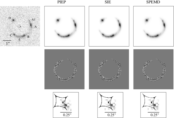
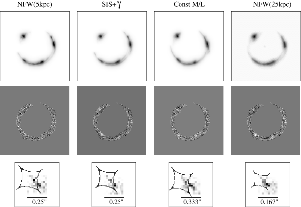
Figure 2: Data and best fitting images for each of the lens models are shown in the upper panels. The residual between the data and model is shown in the centre panels. The corresponding sources, together with the model caustics, are shown in the lower panels.

The results of the modelling procedure are provided in Table 3, and illustrated in Fig. 2. Table 3 lists in successive columns: 1. the name of the lens model, 2. the number of degrees of freedom and $1\sigma$ uncertainty, 3. the $\chi^{2}$ of the best fit, 4. the ratio of the image pixel size to the source pixel size, 5. the area of the caustic, and 6. the relevant best–fit parameters and their errors.

Notwithstanding the above caveats on the comparison of models, the interpretation of these results is relatively straightforward. Two models, the SIS+$\gamma$ and NFW(25 kpc ) models, are strongly rejected on the basis of $\chi^{2}$ alone. Four of the models, the PIEP, SIE, SPEMD, and NFW(5 kpc ) models, provide acceptable fits, with very similar values of $\chi^{2}$. This is not too surprising, since these four models all have very similar mass profiles over the radii of interest. The axis ratio $q_{PIEP}$ can be calculated for equivalent isodensity contours of the PIEP model (for small ellipticities) using equation 3.3.2 of Kassiola & Kovner (1993). This yields $q_{PIEP}=0.77$ in excellent agreement with the SIE/SPEMD. This confirms the expected result that the models are equivalent for large $q$. Finally the constant M/L model lies between the two extremes, producing a $\chi^{2}$ which is rejected with 98% confidence.

Applying the F-test to our models, extends these results. For example comparing the SIE model and the constant M/L model, we have $\Delta\chi^{2}=86$ for a change in number of degrees of freedom of only 2. The significance of this is so great that we may safely rule out the constant M/L model. However the most interesting case is comparison of the SPEMD and SIE models. Here the only change is between fixing the power law exponent to the value $\beta=1$, and allowing it to be a free parameter. The best fit value for the SPEMD model is $\beta=1.08\pm 0.03$ i.e. a small but significant change. The change $\Delta\chi^{2}=4.7$ for $\Delta N=1$ is significant at the $97\%$ level.

Thus, the overall mass distribution in the lens galaxy favours a mass power law which is slightly steeper than isothermal around the Einstein radius. This is important because $H_{0}$ measurements based on lensing time delays are sensitive to the mass power law ($\Sigma\propto R^{-\beta}$) at the radius of the images, with larger values of $\beta$ (i.e. more centrally concentrated mass) leading to larger actual time delays. (This would then be interpreted as smaller value of $H_{0}$ using an isothermal model). Most importantly, we found no strong degeneracy between mass power law $(\beta)$, mass scale $(\Sigma_{0})$ and axis ratio $(q)$ for the SPEMD model– a problem frequently encountered when modelling quasar lenses (e.g. Wambsganss & Paczynski 1994).

The mass enclosed within the critical line is $3.05h_{65}^{-1}\times 10^{11}{\rm\,M_{\odot}}$ for all successful mass models. Using the photometric properties of the lens galaxy from Table 1, we calculate the total projected $M/L_{B}$ inside the Einstein radius to be $4.7h_{65}\pm 0.3$ $M_{\odot}/L_{B\odot}$. This value is smaller than that calculated by KT03 ($5.4\pm 0.8$), however KT03 used a larger Einstein radius (1.34^′′) and the presence of dark matter would make the total $M/L_{B}$ increase with radius. We also note that the constant M/L model, if correct, would require the stellar $M_{*}/L_{B}$ to be $6.8h_{65}$.

Finally, we can infer some qualitative properties of the galaxy’s dark halo in the region of the Einstein radius. The position angle of the mass distribution is almost identical for all successful models and is within a few degrees of the measured position angle for the lens galaxy. The axis ratio of the overall mass profile (q=0.77) is rounder than the axis ratio of the visible galaxy (q=0.69). This indicates that the halo must be substantially rounder than the visible galaxy.

4.2 The source

The inferred morphology of the (unlensed) source, Fig. 2, is particularly interesting. For all the models which provided satisfactory fits the reconstructed source is double, with the smaller component lying inside a fold caustic, and the larger, equally bright, component lying on top of the same fold caustic. This vindicates the use of a non–parametric model for the source. It would be very difficult to determine this solution for the source with a parametric model.

Guided by these results, we created a simple two-component source model, lensing each component separately, and together, through the PIEP lens model, to create the images shown in Fig. 3. The lower left panel shows the image of the inner source component, modelled as a single bright pixel. The middle lower panel is the image of the outer source component, modelled as an elliptical Gaussian. The combination image is shown in the lower right panel. Comparing against Fig. 1, this model shows that features B, C and the brighter spot in A1 are unresolved images of a single source. Features E, A and most of A1 are the image of the extended object which crosses the caustic. Feature D is the combined, barely resolved, image of both components. In their modelling KT03 assumed that the images A, B, C, D are the four images of a single source component. However they were unable to obtain a good fit with their model. This further illustrates the importance of using a suitably detailed source model, also illustrated in Warren & Dye (2003)

In contrast with the models which provide good fits, the source reconstructions for the SIS+$\gamma$, NFW(25kpc), and constant M/L models consist of several fainter blobs or are smeared out and less well defined. There is no a priori reason to believe that the source morphology is simple. However, the complex source geometries evident for the mass models that produce poor fits likely arise from the code’s attempt to compensate for the poor fits by introducing complex structure in the source plane.

Using the reconstructed PIEP source model, the source flux was calculated to be $6.5\times 10^{-17}$ erg s^-1 cm^-2. The overall magnification of the source is 20, hence this is roughly twice the value expected from the Ly${\alpha}$ flux alone (Warren et al. 1996). The discrepancy is probably due to continuum around the emission line which cannot be measured with these observations. Hence, in the following we assume exactly 1/2 of the source flux is contained in the emission line. The source emission line luminosity $L_{Ly{\alpha}}$ is then $4.5\times 10^{42}$ erg s^-1 $h_{65}^{-2}$. Assuming the Ly${\alpha}$ line is not generated by AGN activity, we estimate the number of O/B stars

$$N_{stars}=\frac{L_{Ly{\alpha}}}{E_{Ly{\alpha}}Q_{0}\frac{\alpha^{eff}_{Ly{\alpha}}}{\alpha_{B}}}$$ (1)

required to produce the observed luminosity where $E_{Ly{\alpha}}$ is the energy of a Ly${\alpha}$ photon, $Q_{0}$ is the ionising photon luminosity of a single O/B star from Vacca et al. (1996), $\alpha^{eff}_{Ly{\alpha}}=\alpha_{H_{\beta}}\times(j_{Ly_{\alpha}}/j_{H_{\beta}})(E_{Ly_{\alpha}}/E_{H_{\beta}})$ and the ratio $\frac{\alpha^{eff}_{Ly{\alpha}}}{\alpha_{B}}$ is calculated to be $8.2$ from tables 2.1 and 4.1 in Osterbrock (1989) assuming a temperature of $10^{4}$K, although the ratio depends only weakly on temperature. $Q_{0}$ differs substantially depending on stellar type, ranging from $10^{49.53}$ for an O5 V star to $10^{47.9}$ for a B0.5 V star. Using these values, we estimate $N_{stars}$ to be between $10^{3}$ (all O5 V stars) and $4\times 10^{4}$ (all B0.5 V stars).

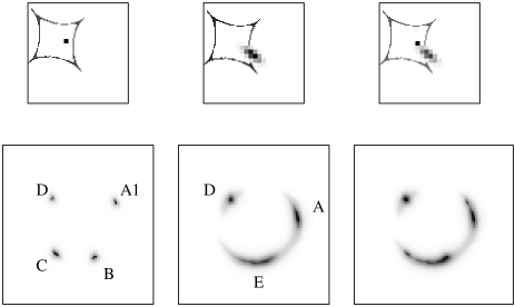
Figure 3: The two components used as the model source (top row) and the corresponding images (bottom row). The linear size of the source plane shown here is 8 times its true size relative to the image plane.

Lens	Model		Image/Source	Area of	Best fitting
Model	$\nu\pm\sqrt{2\nu}$	$\chi^{2}$	pixel size ratio	caustic (arcsec2)	parameters
1. PIEP	719$\pm$38	713.0	2	0.060	b=$1.170\mbox{\mbox{${}^{\prime\prime}$}}\pm 0.004$
					$q=0.917\pm 0.004$
					$\theta_{0}=66.2^{\circ}\pm 0.6$
2. SIS+$\gamma$	719$\pm$38	876.5	2	0.050	b=$1.166\mbox{\mbox{${}^{\prime\prime}$}}$
					$\gamma=0.077$
					$\theta_{0}=60.4^{\circ}$
3. SIE	719$\pm$38	712.0	2	0.060	$b=1.173\mbox{\mbox{${}^{\prime\prime}$}}\pm 0.003$
					$q=0.775\pm 0.005$
					$\theta_{0}=65.9^{\circ}\pm 0.5$
4. SPEMD	718$\pm$38	707.3	2	0.060	$b=1.151\mbox{\mbox{${}^{\prime\prime}$}}\pm 0.007$
					$q=0.76\pm 0.006$
					$\theta_{0}=65.9^{\circ}\pm 0.9$
					$\beta=1.08\pm 0.03$
5. Constant M/L	721$\pm$38	799.2	1.5	0.084	$\kappa_{1/2}=0.453$
6a. NFW(25 kpc )	719$\pm$38	863.1	3	0.020	$\rho_{c}=0.3225$
					$q=0.95$
					$\theta_{0}=64.4$
6b. NFW(5 kpc )	719$\pm$38	721.2	2	0.060	$\rho_{c}=1.133\pm 0.003$
					$q=0.918\pm 0.003$
					$\theta_{0}=66.4\pm 0.8$

Table 3: Results of modelling with six mass models. Models which provide an acceptable fit are shown with $1\sigma$ errors. Models which do not provide an acceptable fit are shown with the ‘best fit’ parameters only. The scale factor $b$ for the SPEMD is the same as the lens Einstein radius only when $\beta=1$.

5 Discussion

KT03 have undertaken an independent study of the ER 0047–2808 system and before discussing the implications of our results we consider the main results of the two studies. KT03 did not find acceptable fits with an SIE+$\gamma$ model and a single component source. Given that they used the lensing data only to measure the total mass interior to the images, KT03 did not pursue more complex models. The model of KT03 required significant external shear and a larger Einstein radius, and consequently their critical curve was larger and flatter and a larger mass was enclosed within it. However, the mass enclosed within a circular aperture of radius $1.17\mbox{\mbox{${}^{\prime\prime}$}}$ is $3.05h_{65}^{-1}\times 10^{11}{\rm\,M_{\odot}}$ for the KT03 model, which agrees well with our models. This result implies that the power-law slope of the mass density published in KT03 ($\gamma^{\prime}$) can be revised upwards by 0.1 at the radius we are considering, leading to the best estimate of the slope to be the isothermal value $\gamma^{\prime}=2.0$ (L. Koopmans, private communication). A simple 1–dimensional calculation of the expected velocity dispersion for a critical radius of 1.17″yields $\sigma=234{\rm\,km\,s^{-1}}$ also in good agreement with the measurement of the corrected central velocity dispersion of $229\pm 15$ kms^-1 from KT03.

Our investigation has identified four mass models [PIEP, SIE, SPEMD and NFW(5 kpc )] which can reproduce the data. While the NFW($5{\rm\,kpc\,}$) model was successful, the inability of a NFW profile with a more realistic scale length (25 kpc ) to reproduce the properties of the ER 0047–2808 system is almost certainly due to the neglect of the baryonic component in the deflector galaxy. The baryonic component is expected to contribute significantly to the total surface mass density within the Einstein radius and the success of the NFW($5{\rm\,kpc\,}$) model is due to the ability of the smaller, much higher density, core to mimic the effect of a significant baryonic contribution at the galaxy centre. It is quite conceivable that inclusion of the baryonic component, and allowance for it’s effects on the dark-matter profile (e.g. Treu & Koopmans 2002), could reconcile the data with the NFW profiles predicted by simulations.

Our modelling has shown that the data alone are able to tightly constrain the slope of the total mass profile of the galaxy. While the elliptical isothermal-like models are all consistent with the data, our models favour a mass profile which is slightly steeper than isothermal ($\Sigma\propto R^{-1.08\pm 0.03}$) around the Einstein radius. The difference in slope corresponds to a $\sim 8\%$ systematic reduction in the value of $H_{0}$ which would be inferred from a time-delay measurement if a pure isothermal model were used.

Three mass models [SIS$+\gamma$, Constant M/L and NFW(25 kpc )] are not capable of reproducing the data. To understand the potential discriminating power of the data we have plotted contours of equal magnification over the data for the successful models (Fig. 4), and unsuccessful models (Fig. 5). The diagrams show the magnification in each region of the image. The critical lines (not shown) lie between the closely spaced contours where the magnification is equal to a factor of 20.

   

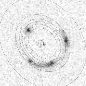
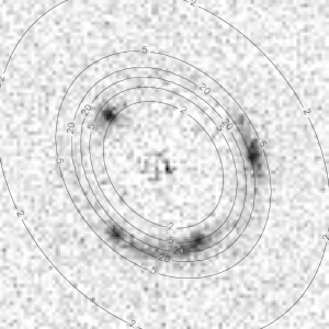
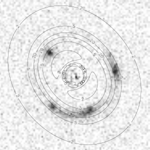
Figure 4: Contours of equal magnification for the successful lens models plotted over the data. From left to right: the PIEP, SPEMD and NFW(5 kpc ) models. Contours show the regions of the image where the magnification is 2, 5 and 20. The critical line for the lens model is between the two contours for magnification 20 in each case. The successful models have remarkably similar critical curves and magnifications around the locations of the images.

Fig. 4 shows the subtle differences between the successful models. The SIE model is indistinguishable from the PIEP model at this image resolution and is not shown. The SPEMD model has a slightly more elliptical critical line compared to the PIEP. In contrast, the NFW(5 kpc ) model has a slightly rounder tangential critical line and some interesting properties near the centre of the lens, with the presence of a radial critical line before the highly demagnified centre of the lens. In spite of this property, the NFW(5 kpc ) lens model does not produce any images near the centre of the lens (given our source position). It is also apparent from Fig. 4 that the magnification of each of the images is virtually the same for the successful models. Images A, B & C are the most highly magnified with a magnification factor $\sim 10$, while image D has a lower magnification of $\sim 4$. Both the similarity in the shape of the magnification contours and of the image magnifications themselves suggest that lens models which have elliptical isothermal–like mass distributions on the scale of the Einstein radius will be able to fit the data (in terms of pure $\chi^{2}$).

Fig. 5 shows that the magnification contours and critical line shape for the unsuccessful models differ significantly from the cases of the PIEP and SIE models. Close examination of the model images show they incorrectly reproduce the brightness and/or location of the bright regions in the data. The SIS$+\gamma$ model produces rounder contours and images B & C are closer to the critical line. This explains why the model does not reproduce the smaller component of the source well, with the consequence that images A1, B & C in the model image are fainter than the data and image C is also incorrectly located. The constant M/L model has magnification contours which are more elliptical than for the PIEP and SIE models. All of the images are further from the critical line and image D in particular is in a region of low ($\sim 2$) magnification, resulting in an image which is the wrong shape (image B is incorrectly located) and considerably fainter than in the data. The NFW(25 kpc ) model has very unusual magnification contours and all of the images are in a high ($\geq 15$) magnification region. This is a consequence of the small area of the caustic in the model, which causes the images to be smeared over several pixels; images B & D are too large while image D is stretched radially more than in the data. Image C is not reproduced as a bright region at all.

   

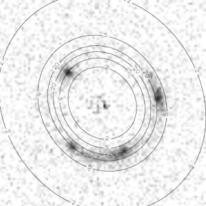
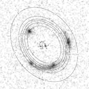
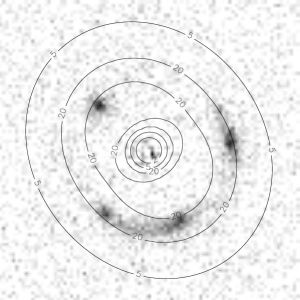
Figure 5: Contours of equal magnification for the unsuccessful lens models plotted over the data. From left to right: the SIS$+\gamma$, constant M/L and NFW(25 kpc ) models. Contours show the regions of the image where the magnification is 2, 5 and 20. The outer magnification 2 contour for the NFW(25kpc) is outside the image region. The critical line for the lens model is between the two contours for magnification of 20 in each case.

Thus, the data are sensitive to both the shape (elliptical vs quadrupole) of the mass distribution and the radial mass density profile. To compare the properties of each model, $\kappa$ and $\beta$ (the local logarithmic slope of the surface mass distribution) at each of the image locations (A,B,C,D) were calculated for each lens model.

Model	$\kappa_{A}$	$\kappa_{B}$	$\kappa_{C}$	$\kappa_{D}$	$\beta_{A}$	$\beta_{B}$	$\beta_{C}$	$\beta_{D}$
PIEP	0.43	0.57	0.44	0.66	1.01	1.00	1.00	1.00
SIE	0.43	0.57	0.44	0.67	1	1	1	1
SPEMD	0.41	0.56	0.42	0.67	1.08	1.08	1.08	1.08
NFW(5 kpc )	0.45	0.49	0.49	0.60	1.34	1.36	1.31	1.30
NFW25	0.68	0.73	0.72	0.81	0.74	0.72	0.72	0.67
Constant M/L	0.21	0.43	0.21	0.59	2.19	1.94	2.18	1.85
SIS + $\gamma$	0.45	0.50	0.49	0.58	1	1	1	1

Table 4: Comparison of $\kappa$ and the local logarithmic slope ($\Sigma\propto R^{-\beta}$) at each image position. The values for images A and D are somewhat uncertain because the images are extended.

The results are shown in Table 4. The table shows that: 1) the properties of the PIEP, SIE and SPEMD are all very similar as expected, and 2) the particular value of $\kappa$ at the image locations is irrelevant, also as expected. The NFW(5 kpc ) model has a local slope which is steeper than the PIEP/SIE and SPEMD models. Hence it has generated a poorer $\chi^{2}$ compared to these models (although still formally acceptable). This is consistent with the data having the ability to distinguish between models based partially upon the local slope of the mass distribution.

This power in the data to distinguish between models raises the question: if the local slope and ellipticity of the mass distribution are important, what exactly is ‘local’? In the context of ER 0047–2808, could we (for example) take the mass inside 0.5″ in the SIE model and replace it with an equivalent point mass with no change in the lensing properties? To quantify this ‘local’ property, the elliptical constant density slab mass models of Schramm (1994) are used. Consider the mass distribution in the lens as a stack of $N$ constant density elliptical slabs with some elliptical radius $r_{e}(i)$ [$r_{e}(i-1)<r_{e}(i)$ for a monotonically decreasing surface mass density]. Each slab has well defined lensing properties and the deflection angle at any point is simply the sum of contributions from all slabs. For a point inside a slab, the deflection is simply that of a homeoidal ellipse. For a point outside the slab, the deflection is equivalent to a point inside a different slab with foci which are at the same point as the original slab, a ‘confocal ellipse’. If a mass distribution is to be distinguishable based on ellipticity and/or radial mass distribution, then the contribution from a slab must not be equivalent to some other slab or point mass. Schramm (1994) gives us the answer for ER 0047–2808. We define the ‘effective ellipticity’ ($\epsilon_{e}$) at a point outside an elliptical slab as the ellipticity of an equivalent confocal elliptical slab. It is easy to show that $\epsilon_{e}\propto(r_{e}/r)^{2}$ for $r>r_{e}$. That is, the effective ellipticity decreases rapidly for points increasingly further away from the outside of the slab. For $r\gg r_{e}$, the slab looks like a point mass, as expected. Hence, for the models presented here where the error on ellipticity (axis ratio) is $\sim 10\%$, the mass inside $\sim 0.03$″ can be replaced with a point mass with no significant change in the lensing properties around the images. In a similar way, slabs with progressively larger radii (larger than the image radius) have progressively lower surface density ($\kappa\propto r^{-1}$ for an SIE), hence their contribution to the overall ellipticity is $\propto r^{-1}$. Again, with an error of $\sim 10\%$ on the measured ellipticity, slabs with a radius $\gtrsim 10\arcsec$ are indistinguishable from a single mass sheet. Using this simple argument, we have defined what ‘local’ means for ER 0047–2808. The implication is that this lens cannot provide information about the mass distribution in the very centre of the galaxy or in the halo very far from the galaxy but there is a substantial range in between which does contribute to the image configuration.

A final noteworthy property of ER 0047–2808 is the lack of necessity of any external shear for a successful lens model. In general, there is likely to be a shear contribution due to the environment. However, the lens is an isolated field elliptical with nearest neighbour $\sim 1^{\prime}$ away (Warren et al. 1999). The shear generated by this object will be small ($\gamma\sim 0.02$) so it is not surprising that no shear was needed to model this system. The large shear required in the model of KT03 was a consequence of having an oversimplified source. We emphasise the importance of using a suitable source model for resolved lenses before conclusions are made about the lens mass distribution.

The combination of this work with that of KT03 has strongly constrained the mass distribution in the lens galaxy, showing it to be very close to isothermal (at least in the region of the images). Well constrained lens models are required for $H_{0}$ measurements using lensing time delays, thus ER 0047–2808 is an excellent candidate for monitoring of supernova events in the source. The lack of external shear also reveals a good deal about the overall mass distribution in the lensing galaxy. Keeton et al. (1998) and Kochanek (2002) have studied the alignment between visible matter and total matter distributions in lens galaxies and found they have an RMS misalignment $<10^{\circ}$. Our result adds weight to their conclusions.

6 Conclusions

We have performed a detailed analysis of ER 0047–2808 using data from WFPC2 on board HST. The data show that the lensed image has four distinct bright regions and two regions of extended emission. We have modelled the image with six different lens models using sophisticated software based on the LensMEM algorithm. The software generates a best-fitting image and reconstructs the source brightness profile using a non-parametric source model.

We have tested the ability of the data to distinguish between a variety of lens models including isothermal, power-law, constant M/L and NFW mass distributions. We find that the ‘canonical’ SIE and PIEP lens models fit the data well and that a power-law model ($\Sigma\propto R^{-\beta}$) favours $\beta=1.08\pm 0.03$, slightly steeper than isothermal. In addition we find that we can fit the data with a mass profile based on the NFW profile, but only when the scale length is too small and central density too high for a dark matter halo expected in a large elliptical galaxy. Conversely, we find that a mass model based on constant M/L or a realistically-sized NFW halo cannot fit the data. We also find that the simple SIS$+\gamma$ lens model does not fit the data despite being an isothermal model. The data are good enough to distinguish between elliptical lens models and the SIS$+\gamma$ which is a first-order approximation of an elliptical model. The difference appears to be in the shape of the critical curve between the elliptical models and external shear model. We have discovered also that the source is actually a double. This has caused problems for models which assume the bright regions in the image come from a single source.

Our results are somewhat different to those of KT03 who found a larger Einstein Radius by $15\%$. However, their model assumed a single source and included a substantial shear component. The mass enclosed by KT03’s model within a $1.17\mbox{\mbox{${}^{\prime\prime}$}}$ aperture is consistent with our model. Our models show that the image locations and brightnesses can be explained neatly with the simple SIE/PIEP mass models and the double source. We calculate the total M/L_B, inside 1.17^′′, to be $4.7h_{65}\pm 0.3$ compared to $5.4\pm 0.8$, at a larger radius of 1.34^′′, in KT03.

We have qualitatively evaluated the behaviour of the lens models around the location of the lensed images by plotting contours of constant magnification. We found that the SIE and PIEP models are indistinguishable for these data and that any elliptical mass distribution with an isothermal-like density profile around the images is likely to be able to fit the data. We found that the lens models which could not fit the data produce images with incorrect magnification and/or location.

Finally, we note that the lens model requires no external shear to explain the data. The well constrained mass distribution, lack of external shear and isolation of the lens galaxy all suggest that ER 0047–2808 is an ideal candidate for further work such as monitoring for supernova events in the source, or making a detailed study of the properties of the galaxy’s dark halo.

References

- Baggett et al. (2002) Baggett S., McMaster M., et al. 2002, “HST WFPC2 Data Handbook Version 4.0”. ed. B. Mobasher, Baltimore: STScI
- Barkana (1998) Barkana R., 1998, ApJ, 502, 531+
- Biretta et al. (2002) Biretta J., Lubin L., et al. 2002, “HST WFPC2 Instrument Handbook Version 7.0”. Baltimore: STScI
- Blandford & Kochanek (1987) Blandford R. D., Kochanek C. S., 1987, ApJ, 321, 658
- Blanton et al. (2001) Blanton M. R., Dalcanton J., Eisenstein D., Loveday J., Strauss M. A., SubbaRao M., Weinberg D. H., Anderson J. E., Annis J., Bahcall N. A., Bernardi M., Doi M., Finkbeiner D., Friedman S., Frieman J. A., York D. G., 2001, AJ, 121, 2358
- Bruzual & Charlot (2003) Bruzual G., Charlot S., 2003, MNRAS, 344, 1000
- Bullock et al. (2001) Bullock J. S., Kolatt T. S., Sigad Y., Somerville R. S., Kravtsov A. V., Klypin A. A., Primack J. R., Dekel A., 2001, MNRAS, 321, 559
- Ciotti & Bertin (1999) Ciotti L., Bertin G., 1999, A&A, 352, 447
- de Vaucouleurs (1948) de Vaucouleurs G., 1948, Annales d’Astrophysique, 11, 247
- Dye & Warren (2004) Dye S., Warren S. J., 2004, ApJ in press. astro-ph/0411451
- Ellithorpe et al. (1996) Ellithorpe J. D., Kochanek C. S., Hewitt J. N., 1996, ApJ, 464, 556
- Fruchter & Hook (2002) Fruchter A. S., Hook R. N., 2002, PASP, 114, 144
- Golse & Kneib (2002) Golse G., Kneib J.-P., 2002, A&A, 390, 821
- Hewett et al. (2000) Hewett P. C., Warren S. J., Willis J. P., Bland-Hawthorn J., Lewis G. F., 2000, in ASP Conf. Ser. 195: Imaging the Universe in Three Dimensions High-Redshift Gravitationally Lensed Galaxies and Tunable Filter Imaging. pp 94–+
- Hewitt et al. (1988) Hewitt J. N., Turner E. L., Schneider D. P., Burke B. F., Langston G. I., 1988, Nat, 333, 537
- Kassiola & Kovner (1993) Kassiola A., Kovner I., 1993, ApJ, 417, 450+
- Keeton (2001) Keeton C. R., 2001, astro-ph/0102340
- Keeton et al. (1998) Keeton C. R., Kochanek C. S., Falco E. E., 1998, ApJ, 509, 561
- Kochanek (1995) Kochanek C. S., 1995, ApJ, 445, 559
- Kochanek (2002) Kochanek C. S., 2002, in The shapes of galaxies and their dark halos, Proceedings of the Yale Cosmology Workshop ”The Shapes of Galaxies and Their Dark Matter Halos”, New Haven, Connecticut, USA, 28-30 May 2001. Edited by Priyamvada Natarajan. Singapore: World Scientific, 2002, ISBN 9810248482, p.62 Mass follows light. pp 62–+
- Kochanek et al. (2000) Kochanek C. S., Falco E. E., Impey C. D., Lehár J., McLeod B. A., Rix H.-W., Keeton C. R., Muñoz J. A., Peng C. Y., 2000, ApJ, 535, 692
- Kochanek et al. (2001) Kochanek C. S., Keeton C. R., McLeod B. A., 2001, ApJ, 547, 50
- Kochanek & Narayan (1992a) Kochanek C. S., Narayan R., 1992a, ApJ, 401, 461
- Kochanek & Narayan (1992b) Kochanek C. S., Narayan R., 1992b, ApJ, 401, 461
- Koopmans & Treu (2003) Koopmans L. V. E., Treu T., 2003, ApJ, 583, 606
- Kormann et al. (1994) Kormann R., Schneider P., Bartelmann M., 1994, A&A, 284, 285
- Krist (1993) Krist J., 1993, in ASP Conf. Ser. 52: Astronomical Data Analysis Software and Systems II Tiny Tim : an HST PSF Simulator. pp 536–+
- Krist (1995) Krist J., 1995, in ASP Conf. Ser. 77: Astronomical Data Analysis Software and Systems IV Simulation of HST PSFs using Tiny Tim. pp 349–+
- Langston et al. (1989) Langston G. I., Schneider D. P., Conner S., Carilli C. L., Lehar J., Burke B. F., Turner E. L., Gunn J. E., Hewitt J. N., Schmidt M., 1989, AJ, 97, 1283
- Miralda-Escude & Lehar (1992) Miralda-Escude J., Lehar J., 1992, MNRAS, 259, 31P
- Navarro et al. (1996) Navarro J. F., Frenk C. S., White S. D. M., 1996, ApJ, 462, 563+
- Osterbrock (1989) Osterbrock D. E., 1989, Astrophysics of gaseous nebulae and active galactic nuclei. Mill Valley, CA, University Science Books, 1989, 422 p.
- Schramm (1994) Schramm T., 1994, A&A, 284, 44
- Sérsic (1968) Sérsic J. L., 1968, Atlas de galaxias australes. Cordoba, Argentina: Observatorio Astronomico, 1968
- Skilling & Bryan (1984) Skilling J., Bryan R. K., 1984, MNRAS, 211, 111+
- Sluse et al. (2003) Sluse D., Surdej J., Claeskens J.-F., Hutsemékers D., Jean C., Courbin F., Nakos T., Billeres M., Khmil S. V., 2003, A&A, 406, L43
- Treu & Koopmans (2002) Treu T., Koopmans L. V. E., 2002, ApJ, 575, 87
- Vacca et al. (1996) Vacca W. D., Garmany C. D., Shull J. M., 1996, ApJ, 460, 914
- Wallington et al. (1996) Wallington S., Kochanek C. S., Narayan R., 1996, ApJ, 465, 64+
- Wambsganss & Paczynski (1994) Wambsganss J., Paczynski B., 1994, AJ, 108, 1156
- Warren & Dye (2003) Warren S. J., Dye S., 2003, ApJ, 590, 673
- Warren et al. (1996) Warren S. J., Hewett P. C., Lewis G. F., Moller P., Iovino A., Shaver P. A., 1996, MNRAS, 278, 139
- Warren et al. (1999) Warren S. J., Lewis G. F., Hewett P. C., Møller P., Shaver P., Iovino A., 1999, A&A, 343, L35
- Warren et al. (2001) Warren S. J., Møller P., Fall S. M., Jakobsen P., 2001, MNRAS, 326, 759
- Wucknitz (2004) Wucknitz O., 2004, MNRAS, 349, 1
- Wucknitz et al. (2004) Wucknitz O., Biggs A. D., Browne I. W. A., 2004, MNRAS, 349, 14