The bottom magnetic field and magnetosphere evolution of neutron star in low mass X-ray binary

Abstract

The accretion induced neutron star magnetic field evolution is studied through considering the accretion flow to drag the field lines aside and dilute the polar field strength, and as a result the equatorial field strength increases, which is buried inside the crust on account of the accretion induced global compression of star crust. The main conclusions of model are as follows: (i) the polar field decays with increasing the accreted mass; (ii) The bottom magnetic field strength of about $10^{8}$ G can occur when neutron star magnetosphere radius approaches the star radius, and it depends on the accretion rate as $\dot{M}^{1/2}$; (iii) The neutron star magnetosphere radius decreases with accretion until it reaches the star radius, and its evolution is little influenced by the initial field and the accretion rate after accreting $\sim 0.01M_{\odot}$, which implies that the magnetosphere radii of neutron stars in LMXBs would be homogeneous if they accreted the comparable masses. As an extension, the physical effects of the possible strong magnetic zone in the X-ray neutron stars and recycled pulsars are discussed. Moreover, the strong magnetic fields in the binary pulsars PSR 1831-00 and PSR 1718-19 after accreting about half solar mass in the binary accretion phase, $8.7\times 10^{10}$ G and $1.28\times 10^{12}$ G, respectively, can be explained through considering the incomplete frozen flow in the polar zone. As a model’s expectation, the existence of the low magnetic field ($\sim 3\times 10^{7}$ G) neutron stars or millisecond pulsars is suggested.

1 Introduction

Recently, the newly discovered double pulsars J0737-3039A and J0737-3039B in the binary system (Burgay et al 2004; Lyne et al 2004; van den Heuvel 2004; Lorimer 2004) have shown that the millisecond pulsar (MSP) possesses the low field and short spin period ($B=7\times 10^{9}$ G, P=22.7 milliseconds) and the normal pulsar possesses high field and long spin period ($B=6\times 10^{12}$ G, P=2.77 seconds), which convinces our previous point of view that MSP is recycled in the binary system where the accreted matter weakened its magnetic field and accelerated its spin (see, e.g., van den Heuvel 2004). Moreover, with the launch of RXTE satellite, the accretion-powered X-ray pulsar SAX J 1808.4-3658 (P=2.49 milliseconds), as well as other five examples (see, e.g., Chakrabarty 2004; van der Klis 2004; Wijnands & van der Klis 1998), and 11 type-I X-ray burst frequency, confirmed as stellar spin frequency, sources have been discovered (see, e.g., Muno 2004; Chakrabarty 2004; van der Klis 2004, 2000), which exhibits the strong evidence that neutron star (NS) in low mass X-ray binary (LMXB) is the progenitor of MSP with spin frequency $\sim$ 400 Hz and magnetic field strength $\sim 10^{8-9}$ G because of the accretion (see, e.g., Wijnands & van der Klis 1998; Chakrabarty 2004).

The origin, structure and evolution of NS magnetic field is still an open problem (see, e.g., Bhattacharya & van den Heuvel 1991; Phinney & Kulkarni 1994; Bhattacharya & Srinivasen 1995; Colpi et al 2001; Melatos & Phinney 2001; Cumming 2004; Blandford et al 1983; Blondin & Freese 1986). In the early stage of discovery of NS, it is believed that NS magnetic field decays due to Ohmic dissipation in the crust. But later calculations of Ohmic dissipation suggest that isolated NS magnetic field may not decay significantly (Sang & Chanmugam 1987), if the field occupies the entire crust, and remains large for more than Hubble time. Although many instructive mechanisms on the isolated NS magnetic decay have been proposed, such as, the crustal plate tectonics model by Ruderman (1991) and Chen & Ruderman 1993, the Hall-drift dominated field evolution (see, e.g., Rheinhardt et al 2004; Jones 2004; Hollerbach & Ruediger 2002; Geppert & Rheinhardt 2002; Rheinhardt & Geppert 2002; Naito & Kojima 1994), the spin-evolution induced magnetic field decay (see, e.g., Konar & Bhattacharya 1997, 1999; Ding et al 1993; Jahan Miri & Bhattacharya 1994; Ruderman et al 1998), etc., there has not yet been a commonly accepted idea on such issue.

The accretion induced NS magnetic field decay has not been paid much attention until 1980’s when Taam and van den Heuvel (1986) presented the NS magnetic field evolution associated with the accretion in the binary system, based on which Shibazaki et al (1989) concluded the simple empirical formula of the field deduction versus the accreted mass. However, it is indicated that the significant decay of magnetic field is achieved only if the neutron star experiences the interacting binary (see, e.g., Verbunt & van den Heuvel 1995; van den Heuvel 1995 and references therein). Furthermore, van den Heuvel and Bitzaraki (1995), from the statistical analysis of 24 binary radio pulsars with nearly circular orbits and low mass companions, discovered a clear correlation between spin period and orbital period, as well as the magnetic field and orbital period. These relations strongly suggest that the increased amount of accreted mass leads to the decay of NS polar magnetic field, and the ‘bottom’ field strength $\sim 10^{8}$ G is also implied, which means that NS magnetic field evolution will stop at some minimum value, $\sim 10^{8}$ G (see also, e.g., Burderi et al 1996; Burderi & D’Amico 1997).

In order to understand the accretion induced field decay, some suggestions and models have been proposed. Based on the accretion buried or screened NS magnetic field guess by Bisnovati-Kogan and Komberg (1974), Zhang et al (1994, 2000) proposed the ferromagnetic crust screen model to interpret the simple inverse correlation between the field deduction and the accreted mass, as declaimed by Shibazaki et al (1989). Moreover, the accretion induced flow and thermal effects to account for the speed-up Ohmic dissipation of NS crust currents are also proposed and studied by several authors (see, e.g., Romani 1990; Geppert & Urpin 1994; Urpin & Geppert 1995). Later on, the diamagnetic screening of NS magnetic field by freshly accreted material is suggested (see e.g. Lovelace et al. 2005), which would be effective above a critical accretion rate $\dot{M}$ of a few percent of the Eddington rate (see, e.g., Cumming et al 2001). More recently, it is calculated that the polar cap widening or the equator-ward hydro-magnetic spreading by the accreted material flowing accounts for the NS magnetic field decay (see, e.g., Konar & Choudhury 2004, references therein; Payne 2005; Payne & Melatos 2004; Melatos & Phinney 2001). Furthermore, the magnetic burial mechanism has been studied in detail analytically and numerically by Payne & Melatos (2004) and Payne (2005) under the assumptions of no instabilities or Ohmic diffusion, where the structure of highly distorted magnetic field and hence the magnetic moment as a function of accreted mass is computed. They find that the deduction of the magnetic moment is inversely related to how much mass accreted and about $\sim 10^{-5}$$M_{\odot}$is required to reduce significantly the magnetic dipole moment.

In this paper, we follow the idea, firstly proposed by van den Heuvel and Bitzaraki (1995), and also by Burderi and D’Amico (1997), that the accretion matter is channeled by the strong magnetic field initially into the two polar patches, corresponding to NS magnetosphere radius of several hundreds of stellar radius, pushes the field lines aside and thus dilutes the polar field strength due to the flow of accreted materials from the polar to the equator. The bottom field should be reached when the accretion becomes all over star, which corresponds to that the NS magnetosphere radius matches the star radius, and in turn it infers the bottom magnetic field to be $\sim 10^{8}$ G.

The paper is organized as follows: in the next section the model is described and the magnetic field evolution equation is derived. Section 3 outlines the applications of the model, including how the NS magnetic field and magnetosphere evolve with the accreted mass, the initial magnetic field and accretion rate, etc.. The discussions are drawn in Section 4, where we summarize the conclusions of model and the observational consequences.

2 Description and calculation of the model

2.1 Dilution of the polar magnetic flux

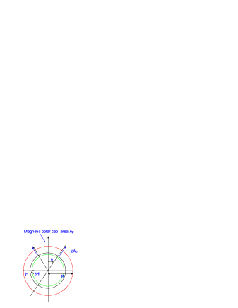
Figure 1: The cross section of the accreted neutron star. $\theta$ is the magnetic polar cap angle of neutron star with radius R. H is the thickness of the crust and $\delta H$ is the expanded immersed depth. $A_{p}$ and $\delta A_{p}$ are the areas of magnetic polar zone and its variation respectively.

For the spherical magnetic slab geometrical structure of accreted NS illustrated in Fig.1, we assume that the magnetic field lines are anchored, completely frozen or incompletely frozen, in the entire NS crust with constant average mass density. The introduction of the spherical topological magnetic polar cap geometry is on account of its important application in describing the kHz QPO mechanism (Zhang 2004), where the spherical magnetic polar cap geometry in Eq.(4) is used and the approximated plane magnetic slab (Cheng & Zhang 1998) is inadequate when the magnetosphere is close to the star surface. Moreover, in the work by Cheng & Zhang (1998) the rate of change of the magnetic polar cap area is roughly performed (see Eq.(5) of that paper), and it should be derived from the magnetic flux conservation as described below. Initially, the magnetic field is sufficient strong, and the accreted matter will be channeled into the polar patches by the field lines. The cumulated accreted matter will be compressed into the crust region through the polar patch or through the surface flow on account of the plasma instabilities (see, e.g., Litwin et al. 2001). However, as a preliminary exploration, we neglect these instability effects on the polar field deduction, and concentrate on the description of the field evolution by the assumed frozen-in crust MHD motions. We suppose the compressed accreted matter to arise the expansion of the magnetic polar zone into two directions, downward and equator-ward. Under the condition of incompressible fluid approximation and the constant crustal volume assumption, as well as the averaged homogenous NS mass density $\rho\sim 10^{14}g/cm^{3}$, where the Ohmic dissipation time scale of field is longer than the flow time scale for sub-Eddington accretion rates (see, e.g., Brown & Bildsten 1998; Geppert et al 1999), the magnetic line frozen motion is assumed and the incomplete frozen motion may appear if the unknown instabilities are taken into effects (see, e.g., Melrose 1986). Therefore, in a particular duration $\delta t$ of accretion with the mass accreting rate $\dot{M}$, the piled accreted mass $\delta M=\dot{M}\delta t$ will arise the expansion of the volume of the magnetic polar zone in the crust, by virtue of the mass flux conservation,

$$(\delta M/2-\rho A_{p}\delta H)\xi=\rho H\delta A_{p}\,,$$ (1)

where $A_{p}$ is the surface area of the magnetic polar zone defined in Eq.(4). The introduced parameter $\xi$ ($0\leq\xi\leq 1$) is an efficiency parameter to express the incomplete magnetic line frozen flow by the plasma instability. In two extremely cases, $\xi=1$ represents that the completely frozen field lines totally drift with the moving mass elements, and $\xi=0$ represents that the completely leaking of plasma makes the field lines not drift with the moving mass elements. The physical meaning of Eq.(1) is clear, $\xi=1$ for instance, that the r.h.s of Eq.(1) is the mass flux toward the equatorial direction and the l.h.s of Eq.(1) is the mass accreted in one polar cap ($\delta M/2$) minus the mass sinked into the NS core. H is the thickness of the crust and $\delta H$/H is the fraction of the thickness dissolving into the core, defined by

$$\frac{\delta H}{H}=\frac{\delta M}{M_{cr}}=\frac{\dot{M}\delta t}{M_{cr}}\,,$$ (2)

where $M_{cr}=4\pi R^{2}\rho H$ is the crust mass. For the standard neutron star structure model, the NS crust mass is only a small portion of the entire NS mass, which is also dependent of the equation of state (EOS) of matter inside NS (see, e.g., Lattimer & Prakash 2004; Baym & Pethick 1975), so $M_{cr}/M\simeq 3H/R\sim 10\%$ is approximately implied. The expansion of the polar zone will dilute the magnetic flux density if the magnetic flux conservation is preserved, that is,

$$\delta(BA_{p})=0\,\,\,\,,\,\,\,\delta A_{p}=-A_{p}\frac{\delta B}{B}\,,$$ (3)

and the area $A_{p}$ of the accretion polar patch can be accurately expressed by the angle $\theta$, which is subtended at the stellar surface between the last closed field line of the NS magnetosphere and the polar axis,

$$A_{p}=\int_{0}^{\theta}2\pi R^{2}\sin\theta^{\prime}d\theta^{\prime}=2\pi R^{2}(1-\cos\theta)\;.$$ (4)

The polar field line can be described by the polar angle $\theta_{r}$ and the position r that satisfies $(\sin^{2}\theta_{r})/r$=constant (see, e.g. Shapiro & Teukolsky 1983, p453), therefore, at the stellar surface, in terms of the NS magnetosphere radius ${R_{{\rm M}}}$,

$$sin^{2}\theta=\frac{R}{R_{M}}\,.$$ (5)

If $\theta$ is small as a case of large magnetosphere radius, we have the approximated relation $A_{p}=\pi R^{2}\sin^{2}\theta=\pi R^{3}/{R_{{\rm M}}}$, as conventionally used (see, e.g. Shapiro & Teukolsky 1983, p453).

${R_{{\rm M}}}$ is related to the Alfven radius ${R_{{\rm A}}}$ by

$$R_{M}=\phi R_{A}\,,$$ (6)

$$R_{A}=3.2\times 10^{8}({\rm cm})\dot{M}^{-2/7}_{17}\mu^{4/7}_{30}m^{-1/7}\,\,\,,$$ (7)

where $\phi$ is a parameter of about 0.5 (see, e.g., Ghosh & Lamb 1979; Shapiro & Teukolsky 1983), but is model dependent (see, e.g., Li & Wang 1999). $m=M/M_{\odot}$ is the NS mass M in units of solar mass, and $\dot{M}_{17}$ and $\mu_{30}$ are the accretion rate in units of $10^{17}$ g/s and the magnetic moment in units of $10^{30}{~{}}{\rm Gcm^{3}}$, respectively.

2.2 The buried magnetic flux in the equatorial zone

With the proceeding of the accretion, the magnetic flux in the polar zone will be diluted and the magnetic flux in the equatorial zone would be increased because of the global conservation of the magnetic flux. However, the new constructed magnetosphere radius is still determined by the new constructed polar magnetic field because the increased equatorial magnetic flux is compressed into the star crust by the global radial accretion flow. Therefore the equatorial strong magnetic field lines are curved and buried inside crust and might be not seen during the accretion phase with the sufficient accretion rate, but it may be seen in the post-accretion phase on account of the Ohmic diffusion. We will try to confirm the above claim through comparing the magnetic flux drifted from the polar zone to the equatorial zone and the magnetic flux compressed into the crust in the equatorial zone.

We substitute Eq.(2) into Eq.(1), and then obtain

$$(2\pi R^{2}-A_{p}){\xi\delta H\over H\delta t}={\delta A_{p}\over\delta t}\,.$$ (8)

After considering Eq.(4) and making the convenient arrangement, we can obtain the ratio between the field line drift velocities in the latitude direction and in the radial direction,

$${v_{\theta}\over v_{{\rm r}}}={\xi R\cos\theta\over H\sin\theta}\;,$$ (9)

with the radial velocity $v_{{\rm r}}=\delta H/\delta t=\dot{M}/4\pi R^{2}\rho$ and the latitude velocity $v_{\theta}=R\delta\theta/\delta t$.

The polar magnetic flux variation rate expelled from the polar zone with the approximated radius $R\sin\theta$ in the latitude direction is

$$\dot{\Phi}_{in}\simeq 2\pi RB\sin\theta v_{\theta}\;,$$ (10)

with $\dot{\Phi}_{in}={d\Phi_{in}\over dt}$, and the equatorial magnetic flux rate compressed into the crust in the radial direction is

$$\dot{\Phi}_{out}\simeq 2\pi RBv_{{\rm ro}}\;,$$ (11)

with $\dot{\Phi}_{out}={d\Phi_{out}\over dt}$ and $v_{{\rm ro}}=\dot{M}/4\pi R^{2}\rho_{o}$, where $\rho_{o}$ is a characteristic mass density at where the matter pressure controls the magnetic pressure. If the non-relativistic neutron in the crust is taken into account, the matter pressure is expressed to be $P_{M}=k\rho^{5/3}$ with k=$5.38\times 10^{9}$ in c.g.s. units (Shapiro & Teukolsky 1983). And the magnetic pressure $P_{B}$ is calculated by the possible maximum permitted magnetic field strength $B_{eqmax}\sim 10^{15}$ Gauss during the accretion compression, exceeding over which the magnetic energy will be released by the soft gamma ray burst triggered by the super-strong magnetic induced crust cracking (see, e.g., Thompson & Duncan 1995), therefore we have,

$$B_{eqmax}^{2}/8\pi=k\rho_{o}^{5/3}\;,$$ (12)

or

$$\rho_{o}\simeq 10^{11}(g/cm^{3})(B_{eqmax}/10^{15})^{6/5}\;.$$ (13)

The ratio between the flux variations in the polar zone and in the equatorial zone can be given if the condition of Eq.(9) is considered,

$${\dot{\Phi}_{in}\over\dot{\Phi}_{out}} = {v_{\theta}{}\sin\theta\over v_{{\rm ro}}}={\xi R\rho_{o}\cos\theta\over H\rho}$$

$$\sim 0.01\xi\cos\theta(B_{eqmax}/10^{15})^{6/5}<1\;,$$

and we find that this ratio is less than unity for the possible parameters, which means that the magnetic flux expelled into the equatorial zone through the latitude direction is much less than that compressed into the crust through the radial direction. Therefore, we can conclude that the magnetic field strength at the magnetosphere-disk boundary will be dominated by the field lines from the polar cap zone, or the magnetosphere radius ${R_{{\rm M}}}$ during accretion will be determined by the polar field. The effective magnetic moment of star decreases because of the motions of field lines, dragged firstly to the equator zone from the polar zone through the latitude motion and then compressed into the crust through the radial motion. Physically, the open field line in the polar zone will be influenced by the latitude flow and little influenced by the radial flow, however the closed field line in the equatorial zone will be dominated by the radial flow. If there exists only the radial flow and no latitude flow, as a case of the magnetosphere reaching the star surface, the polar field will be little changed because the net motion of field lines in the latitude direction disappear. Therefore, with the proceeding of the accretion, the polar field decays and the newly constructed magnetosphere radius is still determined by the decayed polar field strength, or in mathematical terminology the field in the Eqs.(4) and (7) will be same as the polar field described in Eq.(3).

Furthermore, we stress that the above arguments for the field line motion are roughly valid for the purpose of the phenomenological model, however the detail descriptions of the accretion flow, together with the magnetic induction equations, are needed in presenting the NS magnetic structure, which will be the subsequent work elsewhere.

2.3 The polar magnetic field evolution

Furthermore, substituting Eqs.(2), (3)and (4) into Eq.(1), we obtain the magnetic field evolutionary equation as follows,

$$\frac{A_{p}\delta B}{(2\pi R^{2}-A_{p})B}=\frac{-\xi\dot{M}\delta t}{M_{cr}}\,,$$ (15)

or,

$$\frac{(\sqrt{R_{M}}-\sqrt{R_{M}-R})\delta B}{\sqrt{R_{M}-R}B}=\frac{-\xi\dot{M}\delta t}{M_{cr}}\,.$$ (16)

Solving Eq.(15) or Eq.(16) with the initial condition B(t=0)=$B_{o}$, the analytic magnetic field evolution solution is obtained,

$$B=\frac{B_{{\rm f}}}{\{1-[C/\exp(y)-1]^{2}\}^{7/4}}\,,$$ (17)

with $y=\frac{2\xi\Delta M}{7M_{cr}}$, $\Delta{\rm M}=\dot{M}t$, $C=1+\sqrt{1-x_{0}^{2}}\sim 2$ and ${x_{o}}^{2}=(\frac{B_{{\rm f}}}{B_{o}})^{4/7}=R/{\rm R_{M0}}$, where ${\rm R_{M0}}$ is the initial magnetosphere radius and $B_{f}$ is the bottom magnetic field defined by the NS magnetosphere radius matching the star radius, i.e., ${R_{{\rm M}}}(B_{{\rm f}})=R$, therefore,

$$B_{{\rm f}}=1.32\times 10^{8}\,(G)\,(\frac{\dot{M}}{\dot{M}_{Ed}})^{1/2}m^{1/4}R^{-5/4}_{6}\phi^{-7/4}\,,$$ (18)

where $\dot{M}_{Ed}$ is the Eddington accretion rate and $R_{6}$ is the NS radius in units of $10^{6}$ cm. For the reason of simplicity, the usual NS parameter values are set in the later calculations and discussions, such as, m=1.4, $R_{6}=1.5$, $\phi=0.5$ and ${{\rm M_{cr}}}=0.2M_{\odot}$.

3 The applications of the model

3.1 Inverse correlation between the magnetic field and the accreted mass

In the complete magnetic frozen case $\xi=1$ (for the incomplete frozen case, we just take the replacement ${{\rm M_{cr}}}/\xi\rightarrow{{\rm M_{cr}}}$), the magnetic field evolution with the accretion in Eq.(17) can be approximately simplified in the following form by the Taylor serial expansion with the condition $y\ll 1$ or $\Delta{\rm M}\ll 3.5{{\rm M_{cr}}}$,

$$B=\frac{B_{o}}{(1+\frac{4\Delta{\rm M}}{7m_{B}})^{7/4}}\,,$$ (19)

where $m_{B}=0.5{x_{o}}^{2}{{\rm M_{cr}}}=0.5(R/{\rm R_{M0}}){{\rm M_{cr}}}$. For the usual value of bottom field $B_{{\rm f}}\sim 10^{8}$ G and initial field $B_{o}\sim 10^{12}$ G, we obtain $m_{B}\sim 10^{-3}M_{\odot}$. For the high mass X-ray binary (HMXB) or the low mass X-ray binary (LMXB) in the early stage, a little mass is accreted, $\Delta M\sim 10^{-5}M_{\odot}\ll m_{B}$, then Eq.(19) gives,

$$B=\frac{B_{0}}{1+\frac{\Delta{\rm M}}{m_{B}}}\,,$$ (20)

which is just the same form as the empirical formula of the accretion induced field decay proposed by Shibazaki et al. (1989) when fitting the observational data given by Taam and van den Heuvel (1986). Shibazaki et al (1989) find that the best fitted mass constant is $m_{B}$ = $10^{-5}$ – $10^{-3}$ $M_{\odot}$when comparing the theoretical curve of the magnetic field versus the spin period to the observational data. Moreover, the similar mass value of significantly reducing the magnetic dipole moment is also obtained by Payne & Melatos (2004) and Payne (2005) in their self-consistent analytic and numerical calculations of the accretion buried NS polar magnetic field.

If $m_{B}\ll\Delta{\rm M}\ll 3.5{{\rm M_{cr}}}$, then we have the following approximation from Eq.(17),

$$B\simeq 0.8B_{{\rm f}}({\Delta{\rm M}\over{{\rm M_{cr}}}})^{-1.75}\,.$$ (21)

Therefore, Eq.(21) implies that the influence of the initial magnetic field on the magnetic evolution disappears at this stage, and the NS magnetic field is scaled by the bottom field $B_{{\rm f}}$. Furthermore, with increasing of the accreted mass $\Delta{\rm M}\rightarrow{{\rm M_{cr}}}$, the NS magnetic evolution will enter into the ”bottom state”, and $B\rightarrow B_{{\rm f}}$ is obtained. As a detail illustration, the evolution of NS magnetic field versus the accreted mass with various parameter conditions is plotted in Fig.2, where we find that the influence by the initial field on the field evolution exists when $\Delta{\rm M}\ll 0.01M_{\odot}$ and disappears when $\Delta{\rm M}>0.01M_{\odot}$. Finally, the magnetic field evolution will enter into the ”bottom state” when $\Delta{\rm M}\rightarrow{{\rm M_{cr}}}\sim 0.2M_{\odot}$.

3.2 The bottom magnetic field and its correlation to the X-ray luminosity

The conception of bottom field, the possibly arrived minimum field of accreted NS, is evidently proposed by van den Heuvel and Bitzaraki (1995) from the analysis of the magnetic fields of the millisecond pulsars in the binary systems versus the estimated accreted masses, which is explained that the accreted matter pushes and dilutes the polar field lines if the accretion in the channel way and there is no net flow drag effect on the field lines if the spherical accretion in the random way all over star begins. From the point of view of the accretion geometry, the bottom field is reached when the accretion becomes isotropic all over star or the channeled accretion disappears completely (see also, e.g., Burderi et al 1996; Burderi & D’Amico 1997).

Mathematically, as a minimum field, the bottom magnetic field can also be determined by the condition of vanishing the field variation respect to the accreted mass in Eq.(17), i.e.,

$${\delta B\over\delta(\Delta{\rm M})}=0\,,$$ (22)

which gives the magnetic field minimum value to be the bottom field $B_{{\rm f}}$ when the following condition is satisfied,

$$C/\exp(y)-1=0\,,$$ (23)

which can give a critical accreted mass, namely, $\Delta{\rm M}=3.5{}Log(C){{\rm M_{cr}}}\simeq 0.5(M_{\odot})({{\rm M_{cr}}}/0.2)$, after which the bottom field will be preserved whether or not how much extra mass accreted. From the statistics of 24 binary pulsars by van den Heuvel and Bitzaraki (1995), this critical mass is approximately a fraction of $\sim 0.7M_{\odot}$.

In Fig.2, the influence of the accretion rate (luminosity) on the magnetic field is clear that the Eddington luminosity $L_{38}$ ($L_{36}=0.01L_{38}$) corresponds to the bottom field $3\times 10^{8}$ G ($3\times 10^{7}$ G).

The relation between the X-ray luminosity and the magnetic field was first implied from the X-ray spectra of LMXBs by Hasinger and van der Klis (1989), and they found that the Z (Atoll) sources with the Eddington luminosity ($\sim 1\%$ Eddington luminosity) possess the strong (weak) magnetic fields. However, we stress here that the mass accretion rate cannot be exactly inferred from the observations, therefore we conclude that the individual Atoll source possesses a weaker field than that of Z source only when both sources accretes the similar masses and the mass accretion rate of Atoll source is lower than that of Z source.

Moreover, the theoretical analysis also implies the proportional correlation between the magnetic field and the X-ray luminosity (see, e.g., Psaltis & Lamb 1998; Compana 2000). However, the magnetic field and luminosity relation of NS/LMXB $B\propto L_{x}^{1/2}$ was also proposed by White and Zhang (1997) when analyzing the kHz QPO data of the ten LMXB samples under the assumption that the fast spinning neutron stars are close to the spin equilibrium state. In reality, for the specific magnetosphere radius ${R_{{\rm M}}}$ of LMXB, if scaled as $R_{M}\propto(B^{2}/\dot{M})^{2/7}\sim R$, the bottom field should be proportionally related to the accretion rate as $B_{{\rm f}}\propto\dot{M}^{1/2}\propto L_{x}^{1/2}$.

3.3 The effects of parameter $\xi$

If $\xi\ll 1$, the flow dragging effects on the field lines will be low efficiency and the field decay will be slow. In other words, the small $\xi$ causes decreasing the effective accreted mass contributed to the field decay from Eq.(17). The $\xi$ parameter influence can be applicable to the binary pulsars PSR 1831-00 and PSR 1718-19, believed to possess strong magnetic field $8.7\times 10^{10}$ G and $1.28\times 10^{12}$, respectively, after accreted about half solar mass in the binary accretion phase (van den Heuvel & Bitzaraki 1995). Thus we may imagine that the progenitors of both pulsars experience the incomplete frozen plasma flow in their magnetic polar caps, on account of the unknown instabilities, the mechanism of which is still unclear. For these two systems, as drawn in Fig.2, if we set $\xi\sim 0.03$ and $\xi\sim 0.002$, their polar magnetic field can decay to the present values from the assumed initial value $\sim 5\times 10^{12}$ G after accreting half solar mass. While, the introduction of $\xi$ parameter helps us to interpret the sustained strong magnetic field NS after accreting $\sim 0.5M_{\odot}$ in systems PSR 1831-00 and PSR 1718-19 (van den Heuvel & Bitzaraki 1995), and we find a parameter other than the accreted mass to influence on the magnetic field decay, which was expected by Wijers (1997). Moreover, as another example, it was also pointed out by Verbunt et al (1990) that NS in 4U 1626-67 has accreted $\sim 0.1M_{\odot}$ without losing its magnetic field $\sim 10^{12}$ G.

3.4 The NS magnetosphere evolution

The NS magnetosphere radius can be defined by the magnetic field through the condition ${R_{{\rm M}}}/R=(B/B_{f})^{4/7}$,

$${R_{M}\over R}=\frac{1}{1-[C/\exp(y)-1]^{2}}=\frac{\exp(2y)}{2C[\exp(y)-C/2]}\,.$$ (24)

If $y\ll 1$ or $\Delta{\rm M}\ll 3.5{{\rm M_{cr}}}$, then we have the approximated correlation between the magnetosphere radius and the accreted mass,

$${R_{{\rm M}}}=\frac{{\rm R_{M0}}}{1+\frac{4\Delta{\rm M}}{7m_{B}}}\,\,\,or\,\,\,{{R_{{\rm M}}}\over R}=\frac{1}{{R\over{\rm R_{M0}}}+\frac{8\Delta{\rm M}}{7{{\rm M_{cr}}}}}\,.$$ (25)

Furthermore, if $m_{B}\ll\Delta{\rm M}\ll 3.5{{\rm M_{cr}}}$, then we obtain

$${R_{{\rm M}}}/R=0.88({\Delta{\rm M}\over{{\rm M_{cr}}}})^{-1}\,,$$ (26)

which implies that the magnetosphere radius evolution at this stage has nothing to do with any initial conditions and even the X-ray luminosity and only depends on the accreted mass. If the accreted masses are similar for the NSs in LMXBs, their magnetosphere radii would be homogeneous for both high luminosity Z sources and low luminosity Atoll sources. At the last stage of LMXB, if $\Delta{\rm M}\sim{{\rm M_{cr}}}$, then we have ${R_{{\rm M}}}\sim R$. The above analytical conclusions are illustrated in Fig.3, where the magnetosphere evolution versus the accretion mass is plotted, and the accretion rate influence and the initial field influence are taken into account. We find that the magnetosphere radius is proportionally related to field strength and inversely related to the accretion rate at the initial evolution stage, however it has little correlation to the accretion rate (or luminosity) and the initial field when the the accretion mass exceeds over about $0.01M_{\odot}$. In other words, in the late evolution stage, LMXB for instance, the NS magnetosphere radius is scaled by the NS radius, and only depends on the accreted mass.

3.5 The strong magnetic field estimation in the equator zone

With the accretion going, the magnetic field lines are dragged by the accretion flow from the polar cap toward the equator zone, at where they are buried inside the crust by the global compression of the accreted matter or decayed by the possible reconnection of the field lines in the crust. At the last evolution stage of LMXB, the global magnetic flux conservation will help us to estimate the buried equator magnetic field by assuming the initial magnetic flux to equal the final magnetic flux,

$$2\pi R^{2}B_{o}\simeq 2\pi R^{2}B_{{\rm f}}+2\pi RHB_{eq}\,.$$ (27)

For the usual condition $B_{f}\ll B_{o}$, the magnetic field in the equator zone buried inside the crust can be estimated to be $B_{eq}\simeq(R/H)B_{o}$, which is much stronger than the initial field value. Well, it is remarked that this estimation of the equatorial magnetic field is based on the assumption of homogeneously distributed field lines inside the crust. On the detailed magnetic configuration geometry with the accretion, we refer to the analytical and numerical calculations by Payne & Melatos (2004) and Payne (2005), where they compare the magnetic field line structures before/after accretion. As for the real NS mass density profile in the crust, the lower the mass density, the faster the accretion flow velocity. So the more field lines may be cumulated in the low mass density layer, where the field strength would be high but lower than $B_{eqmax}\sim 10^{15}$ Gauss, because the fields as large as this would be unstable in the outer crust and might be able to break the crust at low enough densities (see, e.g. Thompson & Duncan 1995). The observational evidence to support the existence of the strong field may occur in the Type-I X-ray burst sources, which are due to unstable thermonuclear burning of accreted hydrogen and helium on the NS surface to arise the modulation of X-rays at the star rotation, and it is believed that the burst is firstly ignited in the hot spot and then spreads all over star (see, e.g., Strohmayer & Bildsten 2003; Cumming 2004). Therefore, we associate the hot spot with the existence of strong magnetic area. Moreover, the accretion-powered X-ray pulsar SAX J1808.4-3658 (Wijnands & van der Klis 1998; Wijnands et al 2003) hints the magnetically channelled accretion, which may also not exclude the existence of strong magnetic field or the effects of multiple magnetic moment (see, e.g., Psaltis & Chakrabarty 1999). As a plausible application, recently, Cutler (2002) points out that an internal strong magnetic field, while keeping the external dipole magnetic field low, may arise NS mass quadruple to produce that the gravitational radiation braking dominates electromagnetic braking. As a result, NSs in various X-ray binaries and recycled millisecond pulsars could then be detectable by advanced gravitational wave interferometers. In addition, if the details between the accretion and polar field are taken into account, as pointed out by Melatos & Payne (2005), during accretion the NS magnetic field is compressed into a narrow belt at the magnetic equator by material spreading equator-ward from the polar cap. In turn, the compressed field confines the accreted material in a polar mountain, which is misaligned with the rotation axis in general, to produce the gravitational waves. At last, we stress that the magnetic field is not totally decayed but redistributed on account of the accretion flow, and the polar field decreases and the equator field increases but buried inside the crust. The postaccretion diffusion of the suppressed field back to the NS surface may happen in the recycled pulsars as described by Young & Chanmugam (1995). Recent observations, both in the X-ray range of PSR 1821-14 (see, e.g., Becker et al. 2003), and in the radio range (see, e.g., Gil et al. 2002), seem to support the idea of the existence of strong small-scale magnetic field structures at the NS surface, and the further exploration of which has been paid attention recently by a number of authors (see, e.g., Geppert et al 2003; Urpin & Gil 2004).

4 Discussions and conclusions

In summary, the main conclusions of model are listed in the following: (1) The NS polar magnetic field decays in the binary accretion phase, and its evolution experiences the following processes. Roughly speaking, $B\propto\Delta{\rm M}^{-1}$ is the initial field dependent if $\Delta{\rm M}\sim 10^{-4}M_{\odot}$, and then $B\propto\Delta{\rm M}^{-1.75}B_{{\rm f}}$ is independent of the initial field after $\Delta{\rm M}\sim 10^{-2}M_{\odot}$, until the final stage the field B remaining stable at the bottom value of about $B\sim 10^{8}$ G after $\Delta{\rm M}\sim 0.2M_{\odot}$. (2) The bottom field is the accretion rate (or luminosity) dependent as $B\propto\dot{M}^{1/2}$, which concludes that some Z (Atoll) sources with the Eddington luminosity (1% Eddinngton luminosity) may possess the magnetic fields of about $\sim 3\times 10^{8}$ ($\sim 3\times 10^{7}$) G. Therefore, the existence of the low magnetic field ($\sim 3\times 10^{7}$ G) neutron stars or millisecond pulsars is suggested, which needs the confirmation from the future observations. (3) The appearance of the bottom field is nothing to do with the initial field strength, as shown in Fig.2 and Fig.3. (4) On the NS magnetosphere evolution, ${R_{{\rm M}}}\propto\Delta{\rm M}^{-1}$ is the initial field dependent if $\Delta{\rm M}\sim 10^{-4}M_{\odot}$ , and then ${R_{{\rm M}}}\propto\Delta{\rm M}^{-1}$ is independent of the initial field and the luminosity after $\Delta{\rm M}\sim 10^{-2}M_{\odot}$, until the final stage when the magnetosphere radius reaches the star radius. (5) The equator magnetic field increases with the accretion and is stronger than the initial field strength, which is buried inside the crust. Moreover, as known, the occurrence of thermonuclear X-ray bursts in LMXBs requires the NSs to have the fields $B<10^{10}$ G (see Joss & Li 1980), so we may expect the NS in LMXB to accrete $\Delta{\rm M}>0.01M_{\odot}$ and to enter into the homogeneous state, while the field B forgets the initial field $B_{o}$ and only remembers the bottom field $B_{{\rm f}}$. Also, the magnetic field strength distribution of the isolated non-recycled NSs is from $\sim 10^{10}$ G to $\sim 10^{14}$ G (see, e.g., Vranesevic et al 2004; the highest magnetic field can be extended to $10^{15}$ G if the magnetars are included, see Thompson & Duncan 1995), but most MSPs locate in a narrow domain of B field distribution, from $10^{8}$ G to $10^{9}$ G, which seems to support the fact that the NS final magnetic field is not scaled by the initial field $B_{o}$ but scaled by the bottom field $B_{{\rm f}}$. On the characteristic accreted mass $m_{B}\sim 10^{-5}$ – $10^{-3}$ $M_{\odot}$for the significant deduction of the magnetic field, our result is very close to that obtained by Payne & Melatos (2004) and Payne (2005), however the physical meaning of latter is at where the hydrostatic pressure at the base of accretion column overcomes the magnetic tension and the matter spreads over the stellar surface to drag the polar field lines toward the equator. In our model, $m_{B}$ represents the fraction of the crust mass scaled by the ratio of the stellar radius to the initial magnetosphere radius, then the relation of both characteristic masses is still unclear. Finally, although our model has given the observational consistent results, it is a very simple and crude theoretical framework to account for the accretion induced polar field decay. We think that the basic physical idea is clear and has been proposed by a couple of people (see, e.g., van den Heuvel and Bitzaraki 1995; Burderi et al 1996; Burderi & D’Amico 1997) that the transformation from the systematic channeled accretion to the spherical accretion yields the power to decrease the NS polar field strength. However, many physical details have been neglected in the model, such as, the detail of accretion flow and its reaction with the field lines, the plasma instability in the NS melted surface, the details of how the magnetic field is buried in the equatorial zone, the Ohmic dissipation, as well as the Hall-drift effects, etc., therefore the considerations of these will construct our future research explorations.

Figure 2: The magnetic field versus accreted mass diagram with various parameter conditions, the Eddington rate $L_{38}$ and $L_{36}=0.01L_{38}$, and the initial field strengths from $B_{o}=10^{12}$ G to $B_{o}=10^{15}$ G, which are indicated in the figure.

Figure 3: The magnetosphere radius versus accreted mass diagram with various parameter conditions, the Eddington rate $L_{38}$ and $L_{36}=0.01L_{36}$, and the initial field strengths from $B_{0}=10^{12}$ G to $B_{0}=10^{15}$ G, which are indicated in the figure.

References

- (1) Baym, G., & Pethick, C. 1975. Ann. Rev. Nucl. Phys. 25, 27
- (2) Becker, W., Swartz, D. A., & Pavlov, G. G., et al. 2003, ApJ, 594, 798
- (3) Bhattacharya, D., & van den Heuvel, E.P.J. 1991, Phys. Rep., 203, 1
- (4) Bhattacharya, D., & Srinivasan, G. 1995, in X-ray Binaries, eds. W.H.G. Lewin, J. van Paradijs and E.P.J. van den Heuvel,(Cambridg University Press)
- (5) Bisnovati-Kogan, G., & Komberg, B. 1974, Soviet Astronomy, 18, 217
- (6) Blandford, R.D., Applegate, J.H., & Hernquist, L. 1983, MNRAS, 204, 1025
- (7) Blondin, J.M., & Freese, K. 1986, Nature, 323, 786
- (8) Brown, E.F., & Bildsten, L. 1998, ApJ , 496, 915
- (9) Burderi, L., & D’Amico, N. 1997, ApJ , 490, 343
- (10) Burderi, L., King, A.R., & Wynn, G.A. 1996, MNRAS , 283, L63
- (11) Burgay, M., D’Amico, N., Possenti, A., Manchester, R.N., Lyne, A.G., Joshi, B.C., McLaughlin, M.A., Kramer, M., Sarkissian, J.M., Camilo, F., Kalogera, V., Kim, C., & Lorimer, D. 2003, Nature , 426, 531
- (12) Campana, S. 2000, ApJ , 534, L79
- (13) Chen, K. & Ruderman, M. 1993, ApJ , 408, 179
- (14) Cheng, K.S., & Zhang, C.M. 1998, A& A, 337, 441
- (15) Chakrabarty, D. 2004, ”Millisecond Pulsars in X-Ray Binaries”, to appear in Binary Radio Pulsars, ASP Conf. Ser., eds. F.A. Rasio & I.H. Stairs (astro-ph/0408004)
- (16) Colpi, M., Possenti, A., Popov, S., & Pizzolatto, F. 2001, LNP, 578, 440
- (17) Cumming, A. 2004, ”Magnetic field evolution during neutron star recycling”, to appear in Binary Radio Pulsars, ASP Conf. Ser., eds. F.A. Rasio & I.H. Stairs (astro-ph/0404518)
- (18) Cumming A., Zweibel E. G., & Bildsten L. 2001, ApJ , 557, 958
- (19) Cutler, C. 2002, Phys. Rev. D66, 084025 (gr-qc/0206051)
- (20) Ding, K.Y., Cheng, K.S., & Chau, H.F. 1993, ApJ , 408, 167
- (21) Geppert, U., & Urpin, V. 1994, MNRAS, 271, 490
- (22) Geppert, U., Page, D., & Zannias, T. 1999, A&A, 345, 847
- (23) Geppert, U., Rheinhardt, M. 2002, A&A, 392, 1015
- (24) Geppert, U., Rheinhardt, M., & Gil, J. 2003, A&A, 412, L33
- (25) Ghosh, P., & Lamb, F.K. 1979, ApJ, 232, 259; 234, 296
- (26) Gil, J. A., Melikidze, G. I., & Mitra, D. 2002, A&A, 388, 235
- (27) Hasinger, G., & van der Klis, M. 1989, A&A, 225, 79
- (28) Hollerbach, R., & Ruediger, G., 2002, MNRAS , 337, 216
- (29) Jahan Miri M., & Bhattacharya, D. 1994, MNRAS , 269, 455
- (30) Joss, P. C., & Li, F. K. 1980, ApJ, 238, 287
- (31) Konar, S., & Bhattacharya, D. 1997, MNRAS , 284, 311
- (32) Konar, S., & Bhattacharya, D. 1999, MNRAS , 303, 588; 308, 795
- (33) Konar, S., & Choudhury, A. 2004, MNRAS , 348, 661
- (34) Lattimer, J. M., & Prakash, M. 2004, Science, 304, 536
- (35) Li, X. D., & Wang, Z.R. 1999, ApJ , 513, 845
- (36) Litwin, C., Brown, E.F., & Rosner, R. 2001, ApJ , 553, 788
- (37) Lorimer, D. 2004, Nature, 428, 900
- (38) Lovelace, R.V., Romanova, M.M., & Bisnovatyi-Kogan, G.S. 2005, ApJ, 625, 957 (astro-ph/0508168)
- (39) Lyne, A.G., Burgay, M., Kramer, M., Possenti, A., Manchester, R.N., Camilo, F., McLaughlin, M.A., Lorimer, D., D’Amico, N., Joshi, B.C., Reynolds, J., & Freire, P.C.C. 2004, Science, 303, 1089 (astro-ph/0401086)
- (40) Melatos, A., & Phinney, E. S. 2001, PASA, 18, 421
- (41) Melatos, A., & Payne, D. 2005, ApJ, 623, 1044 (astro-ph/0503287)
- (42) Melrose, D.B. 1986, Instability in Space and Laboratory Plasmas (Cambridge University Press, London)
- (43) Muno, M. P. 2004, in Proc. of ”X-ray Timing 2003: Rossi and Beyond”, eds. P. Kaaret, F. K. Lamb, & J.H. Swank, (Melville, NY: American Institute of Physics), (astro-ph/0403394)
- (44) Naito, T., & Kojima, Y. 1994, MNRAS , 266, 597
- (45) Payne, D., & Melatos, A. 2004, MNRAS , 351, 569
- (46) Payne, D., 2005, Ph.D. Thesis, The University of Melbourne
- (47) Phinney, E.S., & Kulkarni, S.R. 1994, ARA&A, 32, 591
- (48) Psaltis, D., & Lamb, F.K. 1998, in Proceedings of the International Conference on Neutron Stars and Pulsars, edited by N. Shibazaki, et al., Universal Academy Press (Frontiers science series; no. 24), p.179
- (49) Psaltis, D., & Chakrabarty, D. 1999, ApJ , 521, 332
- (50) Rheinhardt, M., & Geppert, U. 2002, Phys. Rev. Lett., 88, 1103
- (51) Rheinhardt, M., Konenkov, D., & Geppert, U. 2004, A&A, 420, 631
- (52) Romani, G.W. 1990, Nature, 347, 741
- (53) Ruderman, M. 1991, ApJ, 366, 261; 382, 576; 382, 587
- (54) Ruderman, M., Zhu, T., & Chen, K. 1998, ApJ , 492, 267
- (55) Sang, Y., & Chanmugam, G. 1987, ApJ, 323, L61
- (56) Shapiro, S.L., & Teukolsky, S.A. 1983, Black Holes, White Dwarfs and Neutron Stars. Wiley, New York
- (57) Shibazaki, N., Murakami, T., Shaham, J., & Nomoto, K. 1989, Nature, 342, 656
- (58) Strohmayer, T., & Bildsten, L. 2003, To appear in ’Compact Stellar X-ray sources’, eds. W.H.G. Lewin & M. van der Klis, Cambridge University Press (astro-ph/0301544)
- (59) Taam, R.E., & van den Heuvel, E.P.J. 1986, ApJ, 305, 235
- (60) Thompson, C., & Duncan, R.C. 1995, MNRAS, 275, 255
- (61) Urpin, V., & Geppert, U. 1995, MNRAS, 275, 1117
- (62) Urpin, V., & Gil, J. 2004, A&A, 415, 305
- (63) Verbunt, F. & van den Heuvel E.P.J. 1995, X-ray Binaries, ed. Lewin, W.H.G., van Paradijs, J., & van den Heuvel, E.P.J., Cambridge University Press, pp. 457-494
- (64) van den Heuvel, E.P.J., & Bitzaraki, O. 1995, A&A, 297, L41
- (65) van den Heuvel, E.P.J. 1995, JA&A, 16, 255
- (66) van den Heuvel, E.P.J. 2004, Science, 303, 1143
- (67) van der Klis, M. 2000, ARA&A, 38, 717 (astro-ph/0001167)
- (68) Verbunt, F., Wijers, R.A.M.J., & Burm, H.M.G. 1990, A&A, 234, 195
- (69) Vranesevic, N., Manchester, R.N., Lorimer, D.R., Hobbs, G.B., Lyne, A.G., Kramer, M. Camilo, F., Stairs, I.H., Kaspi, V.M., D’Amico, N., Possenti, A., Crawford, F., Faulkner, A.J., & McLaughlin, M.A. 2004, ApJ , 617, L139
- (70) Wijnands, R., & van der Klis, M. 1998, Nature, 394, 344
- (71) Wijnands, R. et al. 2003, Nature, 424, 44
- (72) Wijers, R. A. M. J. 1997, MNRAS , 287, 607
- (73) White, N.E., & Zhang, W. 1997, APJ, 490, L87
- (74) Young, E.J., & Chanmugam, G. 1995, ApJ, 442, L53
- (75) Zhang, C.M., Wu, X.J., & Yang, G.C. 1994, A&A, 283, 889
- (76) Zhang, C.M. 2000, Intl. J. Mod. Phys., D9, 1
- (77) Zhang, C.M. 2004, A&A, 423, 401 (astro-ph/0402028)