Mapping Large-Scale Gaseous Outflows in Ultraluminous Galaxies with Keck II ESI Spectra: Variations in Outflow Velocity with Galactic Mass

Abstract

Measurements of interstellar Na I $\lambda\lambda 5890,96$ absorption lines in 18 ultraluminous infrared galaxies (ULIGs) have been combined with published Na I data, in order to reassess the dependence of galactic outflow speeds on starburst luminosity and galactic mass. The Doppler shifts reveal outflows of relatively cool gas in 15 of 18 ULIGs with an average outflow speed at the line center of $330\pm 100$ km s^-1 . The relation between outflow speed and star formation rate (SFR), defined by the distribution’s upper envelope over four orders of magnitude in SFR, demonstrates that winds from more luminous starbursts accelerate interstellar gas to higher speeds as roughly $v\propto SFR^{0.35}$. This result is surprising since, in the traditional model for starburst-driven winds, these relatively cool gas clouds are accelerated by the ram pressure of a hot, supernova-heated wind that exhibits weak (if any) X-ray temperature variation with increasing galactic mass. The lack of evidence for much hotter winds is partly a sensitivity issue; but the Na I velocities in ultraluminous starbursts actually are consistent with acceleration by the tepid wind indicating a hotter component is unlikely to dominate the momentum flux. The Na I velocities in the dwarf starburst winds do not reach the terminal velocity of a hot wind at the measured temperature of $kT\sim 0.73$ keV – a result which could be interpreted simply as evidence that the hot superbubbles are too confined in dwarf starbursts to generate a free-flowing wind. A dynamically-motivated scenario, however, is that the dwarf starburst winds simply lack enough momentum to accelerate the clouds to the velocity of the hot wind. Among the subsample of starbursts with well-constrained dynamical masses, the terminal outflow velocities are found to always approach the galactic escape velocity. Motivated by a similar scaling relation for stellar winds, the galactic Eddington luminosity for dusty starbursts is shown to be within the range measured for ULIGs. If radiation pressure on dust grains, coupled to the cool wind, is indeed important for galactic wind dynamics, then feedback will be stronger in massive galaxies than previously thought helping shape the high-mass end of the galaxy luminosity function. Regardless of the nature of the acceleration mechanism in ULIGs, the mass flux of cool gas estimated from these data demonstrates that starburst-driven winds transport significant gas during the assembly stage of field elliptical galaxies – a factor which helps explain the rapid decline in SFR in these systems inferred from elemental abundance ratios.

1 Introduction

Galactic-scale gaseous outflows are ubiquitous in starburst galaxies at all cosmic epochs (Heckman, Armus, & Miley 1990; Pettini et al. 2001; Shapley et al. 2003). Powered by supernova explosions, perhaps with additional help from AGN in very luminous galaxies, these galactic winds transport heavy elements, interstellar dust, and energy into galaxy halos and the intergalactic medium. The significance for galaxy evolution depends on details of the coupling between the available energy, both radiative and mechanical, and the interstellar gas. Observations, which describe this interplay empirically, illuminate the dominant physical processes and provide quantitative constraints for galaxy evolution models.

This paper directly addresses feedback at the high mass end of the galaxy luminosity function via measurements of outflow speeds in ultraluminous starbursts. These new observations of Na I and K I (ionization potential of 5.1 eV and 4.3 eV respectively) interstellar absorption reveal relatively cold gas clouds advected into the outflow at the shear interface between the hot wind and the quiescent gas disk. Material evaporated from these clouds could be the source of the mass-loading required to explain the large X-ray surface brightnesses of galactic winds (e.g. Suchkov et al. 1994; Suchkov et al. 1996; Strickland et al. 2002; Martin, Kobulnicky, & Heckman 2002). Unlike emission lines, absorption lines leave no ambiguity between infall and outflow and are sensitive to extended, low density gas. The results reported here complete a larger effort to describe the low-ionization absorption kinematics over four orders of magnitude in star formation rate (Heckman et al. 2000, luminous infrared galaxies (LIGs); Schwartz & Martin 2004, dwarf starbursts). The observations have little overlap with the Rupke et al. (2002) sample of ULIGs due to different selection criteria (see §2).

Feedback is expected to have a large impact on dwarf galaxies owing to their shallow gravitational potential. It can explain the absence of young galaxies with very low mass, $V_{rot}\lower 2.0pt\hbox{$\buildrel{\scriptstyle<}\over{\scriptstyle\sim}$}\ 10-20$ km s^-1 , after reionization (Barkana & Loeb 1999), the slope of the galaxy luminosity function (Dekel & Silk 1986; Dekel & Woo 2003; Benson et al. 2003), and the mass-metallicity relation among galaxies (Larson 1974). Ablation of the gas in dwarf galaxies by winds from nearby galaxies may help flatten the faint-end of the luminosity function (Scannapieco, Thacker, & Davis 2001).

Observations strongly support the idea that a larger fraction of the metals are removed from dwarf galaxies than massive galaxies. Metallicity measurements from X-ray spectra indicate the hot wind carries the heavy elements produced by the starburst population (Martin et al. 2002). Temperature estimates for the hot gas, i.e. $kT_{x}$, vary little with galactic mass indicating a critical galaxy mass, $V_{c}\sim 130$ km s^-1 , below which most of the hot wind escapes (Martin 1999). Retention of a larger fraction of the metals in more massive galaxies would produce an increasing effective yield with galaxy mass up to this scale where the stellar yield is recovered (Larson 1974; Dekel & Silk 1986; Vader 1987). Although the X-ray data have some significant shortcomings – including a small number of observed objects and a temperature biased towards the densest regions of the hot plasma, the mass-metallicity relation has been measured locally for a complete sample of galaxies. The metallicities increase steeply with mass over the range from $10^{8.5}-10^{10.5}$${\rm~{}M_{\odot}}$$h_{70}^{-2}$ but flatten at $10^{10.5}$${\rm~{}M_{\odot}}$$h_{70}^{-2}$ (Tremonti et al. 2004). The mass scale of the flattening appears to be consistent with the inferred mass scale of metal retention (Garnett 2002). Despite the efficiency of metal ejection, it is not clear whether the total mass loss rates which are of the order of the SFR are sufficient to explain the measured faint-end slope of the galaxy luminosity function, which is flatter than that of the halo mass function (Somerville & Primack 1999).

This paper finds an increase in the velocities of cold clouds with galactic mass suggesting feedback may play a more prominent role in massive galaxies than previously thought, an idea which could be important for several outstanding problems. First, wind velocities are quite important in determining how much of the IGM is polluted (Aguirre 2001). Fast winds from quasars may well deposit more energy into the IGM than starburst winds (Scannepieco & Oh 2004), but they seem unlikely to dominate the metal transport. Second, the galaxy luminosity function cuts off more steeply than the theoretical halo mass function at bright luminosities, and a feedback mechanism physically distinct from that in dwarf galaxies appears to be required to explain both ends of the luminosity function. The mass scale separating these forms of feedback shows up not only in the mass-metallicity relation and X-ray temperatures but also characterizes the galaxy mass scale $\sim 3\times 10^{10}$${\rm~{}M_{\odot}}$ where (1) surface-brightness stops rising with luminosity and mass and (2) less massive galaxies have stellar populations weighted towards younger ages (Blanton et al. 2003; Kauffmann et al. 2003a,b). Any feedback processes invoked to explain these relations must do so without disrupting the Tully-Fisher and Faber-Jackson relations between velocity, i.e. the depth of the gravitational potential, and stellar mass, $V\propto M_{*}^{1/4}$ (e.g. Bernardi et al. 2003), which show no obvious change at this scale (Zwaan et al. 1995; Sprayberry et al. 1995; Dale et al. 1999).

Sample selection and the observational strategy are described in §2. The kinematics and column densities of the nuclear ULIG spectra are presented in §3. Section 4 develops scaling relations between outflow properties and galaxy parameters, including the dynamical state of the merger. The results are shown to challenge the standard model of supernova-driven winds in §5, and the role of radiative acceleration is discussed. §6 summarizes the main results. The second paper in this series (Paper II) describes the surprisingly large spatial extent of Na I absorption, compares kinematics of Na I and H$\alpha$ lines, and discusses the outflowing mass flux in detail.

2 Observations

The spectra presented here extend Na I studies of dwarf starbursts (Schwartz & Martin 2004) and luminous infrared galaxies (Heckman et al. 2000) to ultraluminous galaxies (ULIGs). Targets were chosen from the IRAS (60 micron) 2 Jy sample (Strauss et al. 1992) to have bolometric luminosities greater than $5\times 10^{11}$${~{}\rm L_{\odot}}$, a 60$\mu$m  bump $F_{\nu}^{2}(60\mbox{$\mu${\rm m}})>F_{\nu}(12\mbox{$\mu${\rm m}})\times F_{\nu}(25\mbox{$\mu${\rm m}})$, and declination $\delta>-35\mbox{${}^{\circ}$}~{}$. Spectral observations of 41 of the 64 galaxies satisfying these criteria were obtained. The selection was random unlike the Rupke et al. (2002) sample which pre-selected galaxies with outflows from the 1 Jy survey. The rather large redshift range, $z=0.042$ to $z=0.16$, reflects the paucity of ultraluminous galaxies locally.

Echellete spectra were obtained 2000 September 19-20 and 2001 March 26-29 using ESI on Keck II. The nucleus, identified in R and K band images (Murphy et al. 1996), was placed on the slit. The position angle was usually chosen to include the second nucleus. If the object could not be observed when the parallactic angle swept through the position angle defined by the two nuclei, then an angle closer to parallactic was chosen. The median seeing was 0$\farcs$8 FWHM (full width at half-maximum intensity), which resolves the galactic disks. The 1${}^{\prime\prime}~{}$slit provided a resolution of $\sim 70$ km s^-1 .

The data were reduced using the echelle package in IRAF. Fixed pattern noise was removed from the CCD frames using bias frames and internal quartz illumination frames. Fitted arc lamp exposures (Cu+Ar+Xe) provided a dispersion solution accurate to $\sim 0.15\mbox{~{}\AA}$. The nuclear spectra were traced and extracted, and a sky spectrum extracted from the same slit was interactively scaled and subtracted. The continuum was fitted and normalized to unity in each order. Velocities quoted in the paper are converted to the rest frame and given relative to the Local Standard of Rest.

The primary uncertainty in the outflow velocity of the cool gas is the systemic velocity of the galaxy. This paper focuses on the CO-sample which contains 15 ULIGs with CO velocities from Solomon et al. (1997) and 3 ULIGs with CO velocities from Dr. Aaron Evans (pvt. comm.). The stellar velocities derived from the Mg I lines are fully consistent with the CO velocities although the uncertainties were typically larger. The CO emission was chosen mainly for its insensitivity to extinction and the following dynamical consideration. In galaxy – galaxy mergers, the interstellar gas sinks toward the dynamical center of the merged galaxies as the orbital angular momentum is shed at large radii. The central gas surface density grows to more than 10 times the maximum in the Milky Way, and the ISM is almost entirely molecular (Sanders et al. 1988a). The measured CO velocity therefore provides a better description of the systemic velocity than either HI 21-cm emission, which comes from a larger region, or emission lines from HII regions. For the CO-selected sample described in this paper, the typical accuracy of the CO velocities is $\sim 20$ km s^-1 (Sanders et al. 1988b). In the CO-sample, the minimum luminosity is $6.5\times 10^{11}$${~{}\rm L_{\odot}}$, and the implied star formation rates are several hundred $~{}{\rm M_{\odot}}$ yr^-1 as shown in Table 1. Four of the galaxies are members of the well-studied Bright Galaxy Sample (Sanders et al. 1988b; Sanders et al. 2003).

3 Results

Figure 1 shows the Na I absorption lines in the nuclear spectra. Three features are immediately obvious. First, the doublet lines which are separated by 300 km s^-1  are blended together in all the spectra, so the line widths are much larger than those observed in dwarf starbursts and LIRGs. Second, the total Na I equivalent-widths, see Table 2 are large – ranging from 1 to 10 Å. And, third, the lines are not black at the line center. In this section, we determine the contribution of interstellar absorption to these line profiles, describe the kinematics of the absorbing clouds, and estimate the Na I column density.

3.1 Distinguishing Interstellar and Stellar Na I

Interstellar absorption lines in galactic spectra are formed against a continuum which contains photospheric features. Since the alkali metals are mostly neutral in the atmospheres of late-type stars, such stars present prominent Na I absorption lines. The strength of excited photospheric features, which have no interstellar counterpart, such as the Mg I  $\lambda$5167.32,  $\lambda$5172.68,  $\lambda$5183.60 triplet constrain the contribution of stellar Na I absorption however. In ESI spectra of AFGK dwarf and giant stars, taken in the same manner as the galaxy data, the strength of the NaD doublet relative to the Mg I triplet is well-described by the empirical relation $EW_{NaD}=1/3EW_{MgI}$.

In galaxy spectra, the Mg I lines are blended with other photospheric lines, particularly an Fe I line, because they are broadened by 200-300 km s^-1  FWHM. Figure 2 compares the total Na I equivalent width to the measured equivalent width of the entire Mg I+Fe I complex, rest-frame bandpass from $\lambda 5162\rm{~{}to~{}}\lambda 5189$, in the nuclear ULIG spectra. Excited photospheric features are strongest in IRAS00153+5454, IRAS00188-0856, IRAS17208-0014, IRAS20087-0308, and IRAS23365+3604; but these galaxies also present Na I absorption much stronger than that predicted by the stellar locus. Although the Na I strength for IRAS00262+4251 exceeds the predicted stellar equivalent width by only one standard deviation of the measurement errors, the significant Doppler shift of the lines suggest an interstellar component is present. In Figure2, the upper limit for IRAS19458+0944 is not very restrictive, but the upper limit for the other null detection, IRAS16487+5447, allows only a stellar component.

Table 2 lists the total NaD equivalent width (in the rest-frame $\lambda 5874\rm{~{}to~{}}\lambda 5899$ bandpass) and the fraction inferred to be stellar from the scaling between stellar Na I and Mg I. The stellar contribution to the NaD equivalent width is typically $\sim 10\%$ and will be ignored in the remainder of this paper.

3.2 Interstellar Gas Kinematics

Since the stellar Na I absorption is negligible, the line profiles describe the kinematics of interstellar gas clouds and, if a resolution element is optically thin, the Na I column density at a particular velocity. Doppler shifted absorption components are a robust signature of outflow (for a blueshift) since the absorbing gas must lie on the near side of the galaxy. One obtains no direct information about the location of the absorbing gas along the sightline, however. As discussed in §2, the systemic velocities for the CO-subsample are well determined. The systematic analysis of the Na I absorption presented here draws the robust conclusion that nearly all ULIGs drive fast outflows. For any particular ULIG, the interpretation may be complicated by absorption from tidal debris (e.g. Norman et al. 1996; Hibbard, Vacca, & Yun 2000). Tidal debris, in contrast to starburst-driven outflows, subtend a small solid angle (L. Hernquist, pvt comm), so they are unlikely to be the dominant source of the blue-shifted absorption lines.

3.2.1 Doppler Velocities

The spectral region around Na I $\lambda\lambda 5890,96$ is plotted in Figure 1. Comparison of the systemic velocity, marked by a doublet, to the line profiles reveals that much of the absorbing gas is Doppler shifted to wavelengths shorter than the that of the rest-frame doublet. To describe this dynamic component, a second doublet was fitted while the velocity of the systemic component was held fixed. Although the best fits, which are optically thick, are summarized in Table 3, another set of models with the ratio of the line strengths held equal to the ratio of the oscillator strengths (two-to-one) is provided in Table 4. Comparison of the velocities in these two tables illustrates the maximum systematic uncertainties in the measurements.

Although the fully resolved line profiles might be more complex than these simple Gaussian fits assume, the fitted velocities of the dynamic absorption component, $v_{B}$ in Tables 3 and 4, provide a fair estimate of the mass-weighted outflow velocity. The average fitted outflow velocity is $330\pm 100$ km s^-1 . The uncertainty in $v_{B}$ is only a few  km s^-1  when the profiles show multiple local minima. For example, superposition of the shorter wavelength line from the systemic component and the longer wavelength member of the dynamic component creates three local minima in IRAS08030+5243 and IRAS17208-0014. Two minima and a strong blueshifted line wing require two blueshifted components in IRAS10565+2448 and IRAS18368+3549, and three components were fitted with one component held at the systemic velocity. Fitting smooth, blended line profiles, on the other hand, does not yield a unique solution, and these systems have uncertainties up to $\pm 70$ km s^-1 in $v_{B}$ in Table 3. Selection of a low doublet ratio for the systemic component systematically lowers the fitted velocity of the dynamic component. Comparison of $v_{B}$ in the optically thin limit, Table 4, and the optically thick limit, Table 3, shows the magnitude of the shift is generally negligible. Two exceptions are IRAS00262+4251, where the shift is 100 km s^-1 , and IRAS10494+4424, where the discrepancy is $110\mbox{~{}km~{}s${}^{-1}$}$. In both cases, the model in Table 4, which has the saturated systemic component, is favored. Systematic uncertainties in $v_{B}$ caused by the choice of the doublet ratio are therefore insignificant compared to the magnitude of the outflow velocities.

The maximum outflow velocities were measured where the Na I line profile intersects the continuum. These velocities presumably reflect the terminal cloud velocity significant distances from the starburst. These measurements are not influenced by the details of the line fitting, so they are tabulated with the basic measurements in Table 2. The mean terminal velocity is -750 km s^-1 , which is a few times larger than the galactic rotation speeds. This coincidence is particularly interesting since the escape velocity from the galactic halo is also a few times the rotation speed. The physical meaning of this correlation is explored further in §5.

The He I 5876 emission – present in all spectra except IRAS00188-0856, IRAS03158+4227, IRAS18368+3549, and IRAS20087-0308 – could cause the true terminal velocity to be systematically underestimated. At velocities greater than 729 km s^-1 , absorption from the 5889 Na line is observed at the same wavelength as systemic He I 5876 emission. Three factors indicate this coincidence does not bias the measured terminal velocity. First, the apparent strength of the He I 5876 emission line relative to the upper limits on the He I 4471 line (another triplet with the same lower state as He I 5876) and He I 6678 (the n=3 to n=2 singlet transition) indicates little, if any, of the He I 5876 emission is cancelled by very high velocity Na D absorption. Second, the Na I absorption extends further along the slit than the He I emission in many cases, and Paper II shows similar terminal velocities are measured all along the slit. Finally, the K I $\lambda\lambda 7665,99$ doublet, although a weaker line than Na I, would be expected to trace the same neutral gas. The doublet spacing is 1327 km s^-1  so these lines are not blended. Figure 3 shows that the K I absorption profile closely follow the shape of the Na I profile in IRAS10565+2448 and IRAS20087-0308. Although the K I absorption profile for IRAS15245+1019 reveals an absorption line blueward of the Na I terminal velocity, this candidate high velocity component is not detected in the K I $\lambda 7699$ line (not pictured) and therefore is not the K I $\lambda 7696$ line. The K I lines were not detected in the nuclear spectrum for IRAS17208-0014, and residuals from subtraction of strong OH sky lines prevent an accurate measurement of the K I terminal velocity in IRAS18368+3549. Hence, when the K I doublet was detected, it presented the same terminal velocity as Na I.

In summary, among the 18 galaxies in the CO-subsample, 15 present neutral gas outflows. The galaxies IRAS16487+5447 and IRAS19458+0944 show no (or weak) interstellar Na I absorption. Only the IRAS08030+5243 line profile shows a redshifted component. This outflow fraction of at least 80% in ULIGs, which is higher than the outflow fraction in luminous infrared galaxies and (Heckman et al. 2000) dwarf starbursts (Schwartz & Martin 2004). The most luminous LIGs also presented a higher outflow fraction than lower luminosity LIGs, but the significance of the trend was unclear because the two subsamples were selected differently. The new ULIG data establish a trend of increasing outflow fraction with luminosity. Indeed, all ULIGs may have outflows, and this hypothesis is explored further in §4.3.

3.2.2 Line Widths

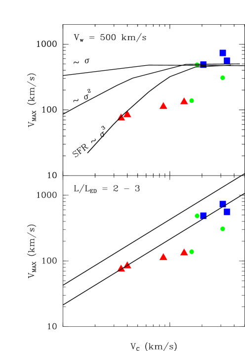
Figure 11: Models for the terminal outflow velocity with respect to the galactic rotation speed. (top) The SFR increases as the cube, square, and first power of the halo velocity dispersion; and momentum from the associated supernovae accelerates cool clouds to the velocity of the hot wind. The models were normalized to the ULIG data such that $SFR=500\mbox{$~{}{\rm M_{\odot}}$~{}yr${}^{-1}$}\ (\sigma/210{\rm~{}km/s})^{3}$, $SFR=500\mbox{$~{}{\rm M_{\odot}}$~{}yr${}^{-1}$}(\sigma/225{\rm~{}km/s})^{2}$, and $SFR=500\mbox{$~{}{\rm M_{\odot}}$~{}yr${}^{-1}$}\ (\sigma/225{\rm~{}km/s})$. (bottom) The luminosity is two or three times the Eddington luminosity where $L_{ED}\equiv 4G^{-1}\sigma^{4}cf_{c}$, and the clouds, assumed to be optically thick at a radius ten times the launch radius, are radiatively accelerated. The radiative acceleration model describes the data as well, and perhaps even better, than than the traditional supernova-driven wind model.

In Table 3, the average line width of the dynamic component is $<\Delta v_{B}>=320\pm 120$ km s^-1 FWHM, much larger than the thermal velocity dispersion of warm neutral gas in galaxies. For comparison, an average sightline through the Milky Way disk detects 6 clouds per kpc in Na I  – each with velocity dispersion $\sim 8$ km s^-1 (Spitzer 1968). Those LIGs with interstellar-dominated Na I absorption also present very broad lines (Heckman et al. 2000). While turbulent motion, particularly at the interfaces between the hot wind and the disk (e.g. Figure 11 in Heckman et al. 2000), is expected to broaden the lines, numerical simulations of bipolar outflows appear to have difficulty producing the large observed velocity range (D. Strickland, pvt comm).

To produce a width of 300-400 km s^-1 , a sightline may need to intersect multiple turbulent sheets or shells, each with distinct bulk motion. Higher resolution spectra (6 km s^-1 in Figure 1 of Schwartz & Martin 2004) support this claim. Along a sightline into the center of M82, the broad Na I doublet, 236 km s^-1  FWHM, is resolved into 5 distinct velocity components, each of width 25 - 79 km s^-1 . And, although the Na I profile remains smooth in NGC 1614, the more optically thin K I lines do break up into multiple components. An important test of dynamical models is to determine, presumably using numerical simulations, whether a more realistic spatial distribution of star formation can generate multiple outflow shells and a broad enough velocity distribution.

The fitted systemic Na I component probes a mixture of stellar absorption and interstellar absorption at the systemic velocity. The formal uncertainties for the widths of the systemic component are significantly larger than those for the dynamic component because the systemic component is generally weak. The average width of the systemic component $\Delta v_{sys}$ is $400\pm 140$ km s^-1 FWHM corresponds to a line-of-sight velocity dispersion, $\sigma=170\pm 60$ km s^-1 . These widths are substantially larger than those measured for stellar-dominated LIGs (Heckman et al. 2000) but lie at the low end of the range measured in ULIG spectra from stellar lines $\sigma_{*}=140-290$ km s^-1  (Genzel et al. 2001). The Na I sample presented in this paper has three galaxies in common with the Genzel et al. sample. In IRAS17208-0014, the stellar velocity dispersion, $\sigma_{*}=229\pm 15$  km s^-1  and $v_{*}=110$ km s^-1 , is subtantially larger than that of the systemic Na I component, $\sigma_{sys}=FWHM/2.35=108$ km s^-1 . However, in IRAS23365+3604 the systemic Na Icomponent, $\sigma_{sys}(\mbox{Na~{}I})\approx 259$ km s^-1  is much larger than the stellar velocity dispersion, $\sigma_{*}=145\pm 15$  km s^-1  and $v_{*}=15$ km s^-1 . The widths are similar in IRAS20087-0308 – $\sigma_{*}=219\pm 14$  km s^-1 , $v_{*}=50$ km s^-1 , and $v_{sys}(\mbox{Na~{}I})=203\mbox{~{}km~{}s${}^{-1}$}$; but this may be largely coincidental considering that the uncertainty in $\Delta v_{sys}$ exceeds 100 km s^-1 . It is not surprising that the fitted Na I systemic components do not appear to be accurate measures of the stellar velocity dispersion – their strength suggests a blend of stellar and interstellar absorption at the systemic velocity.

3.3 Na I Columns

Measurements of the Na I column density in the dynamic component provide a basis for estimating the mass flux of outflowing material per unit area. These measurements differ from absorption measurements using quasars in that the continuum is extended (slit width subtends $\sim 1-2$ kpc of galaxy) and extremely dusty sightlines are excluded from the average. In principle, measurements of the K I lines are more sensitive to column density than the Na I lines, which are shown to suffer from saturation; but subtraction of bright sky lines near K I generally leaves large uncertainties about the K I line strength.

3.3.1 Fitted Models

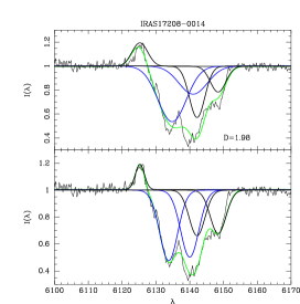
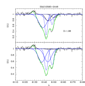
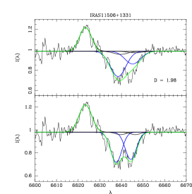
Figure 4: Examples of fitted Na I absorption lines in the optically thin (top panel) and thick (bottom panel) limits. The blue line shows the fitted dynamic component, and the doublet at the systemic velocity is drawn in black. The green line shows the sum of the model components. The optically thick models describe the local minima better than the optically thin models.

The inferred Na I column is only directly proportional to the measured Na I equivalent width if the absorbing material is optically thin. Assuming optically thin clouds, the derived Na I columns range from $\sim 10^{12}$ cm^-2  to a few times $10^{13}$ cm^-2 , see Table 4. Since the optical depth of the stronger doublet member, $\mbox{Na~{}I}\ \lambda 5890$, reaches unity at a column of $N(\mbox{Na~{}I})\approx 3.6\times 10^{13}\mbox{\rm~{}cm${}^{-2}$}\ (v/100{\rm~{}kms~{}}^{-1})^{2}$, the Na I lines are not guaranteed to be optically thin. The columns in Table 4 are good lower limits. The fitted doublet ratios, $D\equiv EW(\lambda 5890)/EW(\lambda 5896)$, in Table 3 illustrate how much larger the true Na I column might be. The fit statistic was improved for every galaxy when the doublet ratio was allowed to decrease from the optically thin limit, $D=1.98$. Figure 4 shows that the thick models do a better job of fitting the structure in the line profiles. Optically thin fits cannot be ruled out for the smooth, featureless profiles in IRAS00262+4251 and IRAS20087-0308, but there is no obvious reason to expect these systems to be optically thin when the better constrained fits all indicate optically thick outflows toward the nucleus.

3.3.2 Cloud Covering Factor

Optically thick clouds that cover the continuum source would leave absorption lines completely black at the line centers. None of the lines in Figure 1 are black at line center. The conclusion that the Na I lines are saturated in many, if not all, of these galaxies directly implies that the absorbing clouds do not completely cover the continuum source.

In the limit of large optical depth, the cloud covering factor $C_{f}$ is simply $\approx 1-I_{5890}$, where $I_{5890}$ is the residual intensity in the  $\lambda$5890 line. The covering factors listed in Table 2, which use the $I_{5890}$ value fitted in Figure 1, indicate that 25% of the visible continuum source is covered by the clouds on average. The covering factors show a relatively large range, however, from 10% in IRAS16090-0139 and IRAS00262+4251 up to nearly 70% in IRAS15245+1019.

When optically thick gas only partially covers the continuum source, the measured equivalent width will be insensitive to the Na I column density and will be primarily determined by the product of the covering factor and the line-of-sight velocity dispersion. Figure 5 shows that the FWHM of the dynamic component is not correlated with the total Na I equivalent width. It does not correlate with the EW of the dynamic component either. The bottom panel of Figure 5 shows that the lowest equivalent width systems all present low covering factors, and that large covering factors are only found in galaxies presenting very high Na I equivalent width. A large covering factor of cool, outflowing gas may partially reflect the viewing angle, but the analysis of §4.4 indicates temporal variations are also important.

3.3.3 Conclusions about Column Densities

Seven of the ULIGs show extremely strong NaD equivalent width ($EW_{o}>7\mbox{~{}\AA}$); they are IRAS00188-0856, IRAS08030+5243, IRAS10565+2448, IRAS15245+1019, IRAS17208-0014, IRAS18368+3549, and IRAS20087-0308. The optically thin models generally give larger Na I columns in the galaxies with larger Na I equivalent widths. The association is not exactly one-to-one however. For example is IRAS15245+1019 is 5th in total EW but 3rd in total column because the particularly large Doppler shifts leave very little absorbed flux near the systemic velocity. Hence, the fraction of the total equivalent width provided by the systemic component is particularly low in this galaxy. The relative equivalent widths of the dynamic and systemic components can be ambiguous when the profile is smooth. Among the 7 largest equivalent width systems, this happens in IRAS20087-0308 and IRAS00188-0856 where fits with more absorption at $v_{sys}$ are clearly allowed.

Some of the profiles absolutely require very large fitted columns. Focusing on the systems with the largest equivalent width again, one finds that the systemic component has to be very weak in IRAS10565-2448, IRAS18368+3549, and IRAS15245+1019. Similarly, the systemic component is strong but maxed out in the fits to IRAS17208-0014 and IRAS08030+5243. In summary, freeing the doublet ratio raises the Na I column to $N(\mbox{Na~{}I})\sim 10^{14}$ cm^-2  to $10^{15}$ cm^-2  in galaxies for which the optically thin model indicated large columns. The correction, however, has little impact on the columns in weaker systems,$N(\mbox{Na~{}I})\times 10^{12}$ cm^-2  since it is not linear and therefore increases the range of measured Na I column densities.

4 Discussion

The absorption measurements presented here trace gas clouds with a significant neutral component. As discussed above, the absorbing material is thought to be disk gas entrained in a hot supernovae heated outflow. The X-ray observations are biased by conditions in the highest density regions of hot component and do not necessarily reveal the hottest (lowest density) regions of the hot outflow (Strickland & Stevens 2000), but they do show that most of the shock heated mass can escape from dwarf galaxies with velocities less than 130  km s^-1 (Martin 1999; Martin 2004). More of the shock heated gas remains bound in larger galaxies, and this differential feedback contributes to the flattening of the slope of the faint-end of the luminosity function. No direct measurements of the kinematics are currently possible in the hot phase. Since the clouds absorbing in Na I are presumably embedded in this medium, it is possible to learn about the wind fluid itself via the motions of the clouds.

4.1 Outflow Mass

The inferred H column associated with a sightline depends on the chemical abundance, dust depletion, and ionization state of the gas. Assuming solar abundances in the ULIGs, the H column is

$$N_{H}=4.90\times 10^{20}~{}{\rm cm}^{-2}\left(\frac{N_{NaI}}{10^{14}{\rm~{}cm}^{-2}}\right)\left(\frac{d_{Na}}{10}\right)\times$$

$$\left(\frac{N(Na)}{N(NaI)}\right).$$ (1)

Heckman et al. (2000) argue, based on parameters of Galactic clouds, that the depletion of Na onto dust grains, $d_{Na}=(N(Na)_{gas}+N(Na)_{dust})/N(Na)_{gas}$, is likely a factor $\sim 10$, and the ionization correction, e.g. $N(Na)/N(NaI)$, could be as much as a factor of 3 to 10.

The nuclear sightlines sample a small region of each galactic halo, so extrapolating these column densities to masses is very sensitive to the chosen area.

Observations of the absorption-line profiles at multiple positions across the galactic disks of ULIGs, presented in Paper II, indicate that some outflows cover more than 10 kpc of the host galaxy. Taking a fiducial radius of $\sim 5$ kpc for purposes of illustration here, the mass of clouds, $M\sim N_{H}A\mu m_{p}$ or

$$M_{c}\sim 1.08\times 10^{8}\mbox{${\rm~{}M_{\odot}}$}\left(\frac{N_{Na}}{10^{14}{\rm~{}cm}^{-2}}\right)\left(\frac{d_{Na}}{10}\right)\times$$

$$\left(\frac{N(Na)}{N(NaI)}\right)\left(\frac{R}{5~{}{\rm kpc}}\right)^{2}.$$ (2)

are applied. The kinetic energy carried by the cold clouds, $1/2Mv^{2}$, is

$$E\sim 1.71\times 10^{56}~{}{\rm ergs}\left(\frac{N_{NaI}}{10^{14}\mbox{\rm~{}cm${}^{-2}$}}\right)\left(\frac{d_{Na}}{10}\right)\times$$

$$\left(\frac{N(Na)}{N(NaI)}\right)\left(\frac{R}{5~{}{\rm kpc}}\right)^{2}$$

$$\left(\frac{v}{400{\rm~{}km~{}s}^{-1}}\right)^{2}.$$ (3)

The enormity of these quantities is perhaps most appreciated when the mass loss rate, $\dot{M_{c}}=\Omega r^{2}\rho v=\Omega r\mu m_{H}N_{H}v$ or

$$\dot{M_{c}}=141\mbox{$~{}{\rm M_{\odot}}$~{}yr${}^{-1}$}\left(\frac{N_{H}}{4.9\times 10^{20}{\rm~{}cm}^{-2}}\right)\left(\frac{R}{5~{}{\rm kpc}}\right)\times$$

$$\left(\frac{v}{400~{}{\rm km~{}s}^{-1}}\right)\left(\frac{\Omega}{4\pi}\right),$$ (4)

is compared to the SFR. For example, applying these expressions to IRAS10565+2448 indicates a mass flux in cool gas of $\sim 300\mbox{$~{}{\rm M_{\odot}}$~{}yr${}^{-1}$}$, which is similar to the SFR of 190$~{}{\rm M_{\odot}}$ yr^-1. Paper II presents spatially resolved line profiles and more detailed estimates of the mass loss rates, but this example illustrates the potential importance of the cold outflows. If they can be sustained for even 10 Myr, several billion solar masses of interstellar gas is transported out of the disk thereby starving the starburst for fuel.

4.2 Variation of Outflow Velocity with Galactic Mass

One of the principal motivations for this study and that of Schwartz & Martin (2003) was to investigate how outflow velocities scale with galactic mass. Surprisingly, Heckman et al. (2000) found no correlation between outflow velocity and galactic rotation speed, or starburst luminosity. Simple extrapolation of this result would imply dwarf galaxies completely dominate intergalactic enrichment. High-resolution Na I spectra of seven dwarf starburst galaxies, however, revealed outflows in three sytems; but the velocities, $-25$ km s^-1 to -35 km s^-1 , were much lower than those in the LIGs (Schwartz & Martin 2004). Provided their luminosities are dominated by the starburst rather than a quasar, the ULIGs have star formation rates from 190 - 750 $~{}{\rm M_{\odot}}$ yr^-1, which (by definition) is higher than that for LIGs which drop down to about 10$~{}{\rm M_{\odot}}$ yr^-1. Outflow velocities, all measured in Na I absorption, can now be compared over four orders of magnitude in SFR.

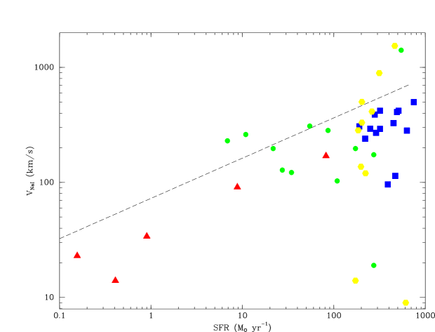
Figure 6: Outflow velocities at line center vs galactic star formation rate. The new data, 1 Jy ULIGs (Rupke et al. 2002), LIGs (Heckman et al. 2000), and dwarf starbursts (Schwartz & Martin 2004) are denoted by squares, hexagons, circles, and triangles, respectively. These starburst systems represent the highest surface brightness objects in their luminosity class and are thought to define the maximum outflow velocities reached. The dashed line represents the fitted upper envelope when a simple model for projection effects is applied (see text in §4.2 for detailsR).

In Figure 6, these velocities exhibit scatter at a given SFR, but the upper envelope of the velocity distribution clearly rises with SFR. The galaxies plotted in Figure 6 are all selected for their starburst activity. They represent the highest areal star formation rate at a given luminosity and, presumably, the strongest outflows. Velocity measurements in normal galaxies would fill in the low velocity regions of Figure 6. The observed velocity spread may reflect mainly projection effects, as argued in §4.3. In this case, a linear least squares fit to these data, $\log(V)=(0.35\pm 0.06)\log(SFR)+1.56\pm 0.13$ where the outflow velocity $V$ is in  km s^-1  and the SFR has units $~{}{\rm M_{\odot}}$ yr^-1, should describe the slope of the upper envelope in Figure 6.

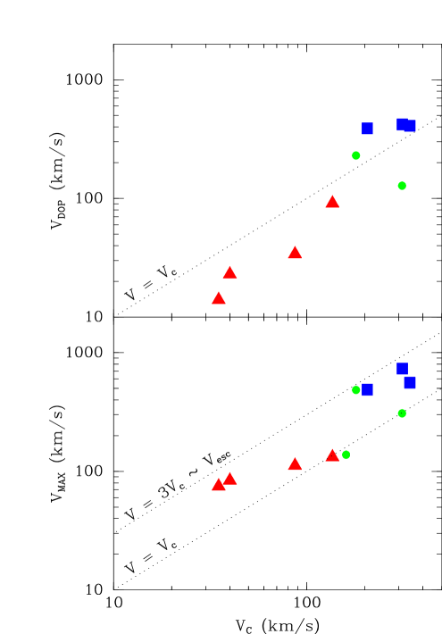
Figure 8: (top) Outflow velocity at Na I line center versus galactic rotation speed. (bottom) Terminal Na I velocity versus galactic rotation speed.

The dynamical masses of the galaxies are not as well constrained as the star formation rates but provide a more fundamental quantity for comparing the outflow velocities. The three dwarf galaxies have rotation speeds of 35 km s^-1 (NGC 1569; Stil & Israel 2002 ), 40 km s^-1 (NGC 4214; Walter et al. 2001), and 87 km s^-1 (NGC 4449; Hunter, vanWoerden, & Gallagher 1999) and are clearly less massive than the LIGs and ULIGs. Ultraluminous activity, on the other hand, requires a large amount of gas, $M_{gas}\sim 10^{10}$${\rm~{}M_{\odot}}$, and a major merger (Borne et al. 2000). The expectation of massive progenitor galaxies is confirmed by measured rotation curves and stellar velocity dispersions for three ULIGs in this sample (Genzel et al. 2001). In the LIG luminosity range, however, the SFR is a poor surrogate for dynamical mass. The LIG subsample for which Heckman et al. had rotation curves has a mean rotation speed of $199\pm 45$ km s^-1 , which is less than that of the Galaxy indicating some LIGs are not massive enough to become ULIGs. Some fraction of LIG progenitors, however, are likely major mergers that were ultraluminous near perigalactic passage but faded during the long journey through apogalacticon. This idea is supported by (1) the significant overlap in CO masses between LIGs and ULIGs (Gao & Solomon 1999), (2) the revived starburst activity suggested by the bimodel distribution of ULIG merger ages (Murphy et al. 2001), and (3) the wider mean separation of LIGs relative to ULIGs. Unfortunately, most of the LIGs with measured rotation speeds are highly inclined disks for which no outflow was detected by Heckman et al. (2000). Consequently, rotation curves are only available for two of the LIGs shown in Figure 6. Considering the paucity of data and poorly determined inclination corrections for the outflow velocities, these results should be taken as preliminary. Nonetheless, the combined data do indicate a steep rise in outflow velocity with rotation speed, illustrated in Figure 8. This result is potentially of fundamental significance, so it will be important to obtain more rotation curves. For the galaxies without rotation curves, rough circular velocities estimated from line-widths yield few velocities above than the preliminary relation, so Figure 8 may actually provide a reasonable description of the upper envelope.

Absorption lines are ideal probes of the kinematics of extended low density gas, so it is not surprising that outflows were one of the first features identified in spectra of high-redshift galaxies, whose optical spectra include the plethora of strong absorption lines in the rest-frame ultraviolet bandpass. The choice of systemic velocity is critical when comparing outflow speeds. In particular, Ly$\alpha$ emission is often seen redshifted relative to stellar features due to resonance scattering off the receding side of the flow and therefore makes a poor zeropoint. Among Lyman-Break-selected galaxies at $z\sim 3$, the galaxy MS1512-cB58 has the highest quality spectra due its large lensing amplification. The measured SFR, 40$~{}{\rm M_{\odot}}$ yr^-1, and outflow velocity, 255 km s^-1 (Pettini et al. 2002) place it right on the average relation for nearby LIGs. The high-redshift objects with bolometric luminosities in the ULIG range are selected in the sub-mm (Ivison et al. 2000). Rest-frame ultraviolet spectra show median offsets between the H$\alpha$ velocity and low-ionization ultraviolet resonance absorption lines of $\sim 650$ km s^-1 at luminosities of a few hundred $~{}{\rm M_{\odot}}$ yr^-1(S. Chapman, pvt comm), which place them in the same part of Figure 6 as the local ULIGs. Outflows from high-redshift galaxies therefore appear to obey the same scaling relations as winds from local starbursts.

Neutral outflows are not only faster in more massive galaxies, but their terminal velocity also appears to increase almost linearly with the galactic rotation speed. The bottom panel of Figure 8 shows the terminal velocities are always 2 to 3 times the rotation speed. This normalization is particularly interesting since the escape velocity is $\sqrt{2}$ (minimum) to 3.5 (isothermal halo extending to 100 kpc) times larger than the circular velocity. The estimated escape velocities are roughly 100 km s^-1 , 400 km s^-1 , and 900 km s^-1 in dwarf starbursts, LIGs, and ULIGs respectively. The proximity of the upper envelope in Figure 6 to these values provides important information about the dynamics of the outflows and is discussed further in §5.

4.3 Velocity Variations from Sightline Orientation

X-ray and optical imaging of nearby starburst galaxies indicate the outflow axis is aligned perpendicular to the disk plane. Identical bipolar outflows viewed at random angles will yield a large range of measured Na I velocities, so it is interesting to examine whether the fastest outflows might be found in systems with galactic disks oriented nearly face-on to our sightline. This hypothesis is supported by the paucity of outflows in the edge-on sample of LIGs (Heckman et al. 2000). Inclination is only well defined for a few of the ULIGs due to both the lack of high-resolution imaging and the on-going merger. NICMOS images of IRAS17208-0014 and IRAS10565+2448 show these disks are oriented close to face on (Scoville et al. 2000), and the outflow velocities in both are among the largest measured at comparable SFR. If large outflow velocities are purely an inclination effect, then ULIGs like IRAS23365+3604 and IRAS18368+3549 must also be observed nearly face-on, which is not inconsistent with their appearance in ground-based images. Large axial ratios indicate two ULIGs are likely viewed edge-on. Of these IRAS03521+0028 has very weak Na I, and IRAS11506+1331 has little net outflowing material in Na I. Inclination therefore appears to have something to do with observed velocity spread at a given SFR.

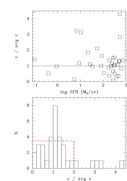
Figure 7: (top) Distribution of outflow velocities normalized by the mean at a given star formation rate. (bottom) Histogram of top panel for all values of the SFR. The expected number of galaxies with outflow velocity between $v_{n}$ and $v_{m}$ is $N(v_{n},v_{m})=N(v_{max},0)\frac{v_{n}-v_{m}}{2.0<v>}$ illustrated in the bottom panel by a dashed line. The four objects with $v>>v_{max}$ present a significant departure from the model.

To examine inclination effects quantitatively, consider a simple model where the flow is perpendicular to the disk plane. The average polar viewing angle is $i=57\mbox{${}^{\circ}$}~{}$, and the average projected velocity is $0.5v_{max}$. It follows that, at any particular SFR, the true outflow velocity is twice as large as the average projected outflow velocity measured. Multiplying the fitted $v_{B}~{}vs~{}SFR$ relation by 2.0 yields the dashed line sketched in Figure 6. This estimate of the de-projected outflow velocity describes the upper envelope adequately for all but a few, particularly luminous, objects. The distribution of observed velocities about the mean is shown in Figure 7, where the data were divided by the mean velocity at the appropriate SFR and then binned according to their deviation from the mean. The naive, planar flow model predicts a constant number of galaxies with increasing $v/v_{avg}$ up to $v_{max}=2.0v_{avg}$. The data show more galaxies with outflow speeds near the average than predicted, but this may be consistent with a more realistic representation of the wind geometry where the velocity field has a radial component. Projection effects, however, fail to explain the high velocity tail in the distribution, and this shortcoming is further discussed in §5.

4.4 Merger Sequence

In addition to inclination, the other property that clearly varies among the ULIGs is the dynamical age of the merger, which is constrained by morphology (Murphy et al. 2001). Visual and near infrared imaging of ULIGs drawn from the 2 Jy sample show galaxy pairs, tidal tails, and double nuclei (Murphy et al. 1996). Inspection of these images allows some ULIGs to be identified as first passage, late passage, and fully merged. The ESI spectra resolve a number of nuclei, previously classified as single nuclei, into double nuclei. The outflow velocities do not correlate with dynamical age, but the strength of the wind does show some interesting trends that may provide some insight about the role of the winds in the ULIG-QSO transition.

Highly eccentric orbits are required to create an intense, short-lived disturbance which centrally concentrates the interstellar gas, so the galaxies pass rapidly on their first encounter. Short tidal features are one signature of first passage because it takes time for tidal features to grow. Disk-like morphology also indicates not enough time has elapsed for the stellar orbits to reflect the transferred orbital energy. Of the 18 ULIGs discussed in this paper, five are plausibly on their first passage. Short tidal features are seen in IRAS10565+2448, IRAS11506+1331, IRAS19458+0944, and IRAS17208-0014, and the debris in IRAS00153+5454 is confined to the region around the distorted disks. These are all double nuclei systems. Of the five strongest Na I lines (i.e. equivalent width $>7$ Å), two are found among these 5 galaxies. The other three strong lined systems are caught during the second pass. In Figure 9, these two are pictured along with their line profiles to represent the first-pass mergers.

The duty cycle of the ultraluminous phase must be $\lower 2.0pt\hbox{$\buildrel{\scriptstyle<}\over{\scriptstyle\sim}$}\ 20\%$ because the estimated dynamical timescales for the mergers, $5\times 10^{8}$ yr to $15\times 10^{8}$ yr (Murphy et al. 1996), exceed the gas consumption timescales, $\sim 10^{8}$ yr. Most of the time between passages is spent near apogalacticon where the galaxies are unlikely to be ultraluminous. None of the systems with strong winds are found in a widely separated phase. The lack of tails and largely symmetric structure in IRAS00188-0856, IRAS16487+5447, and IRAS19297-0406 point toward a stage just before the second encounter. The relatively large separations 20.2 kpc, 5.3 kpc, and 4.4 kpc are consistent with this picture. Their Na I absorption, Figure 9, is quite weak, comparable to Na I line strengths in LIGs. These observations indicate the wind strength decreases when the galaxies are far apart between encounters. Three systems in the ULIG subsample can be identified with the second (or nth) passage by their double nuclei, large tidal structures, and/or more spheroid-like than disk-like structure. The identification as 2nd-passage systems is most secure for IRAS15245+1019, IRAS20087-0308, and IRAS18368+3549, which have particularly long tidal tails. All three of these ULIGS present very large Na I equivalent widths.

The nuclei were not resolved in 7 systems, and the interstellar Na I lines are generally weaker in these single nuclei systems. The most recently merged systems still present large, diffuse tidal structures as seen in IRAS00262+4251, IRAS03521+0028, IRAS16090-0139, and IRAS23365+3604. The line strengths are moderately strong falling between those of systems on the nth-passage and the most advanced mergers in this sample. The other two systems, IRAS03158+4227 and IRAS08030+5243, present quite symmetric and much fainter tidal debris; and the interstellar Na I absorption is weak. These results suggesting the wind is dying down in the older systems.

The combined small size of this ULIG sample and the large variations in the accuracy of the dynamical ages estimates makes a robust statistical analysis unfeasible. However, this preliminary exploration strongly suggests that the strongest winds are found in systems near perigalactic passage. Furthermore, the winds appear to weaken when (1) the galaxies are far apart and (2) the merger is complete. The starburst probably dies down due to growing scarcity of gas. Further investigation may determine whether the gas is simply consumed, removed by the starburst, or removed by a nascent AGN-driven outflow.

5 Acceleration of the Cool Wind

Consistency between the X-ray and Na I measurements is an important test of the standard dynamical model for starburst winds, which assumes a thermally-driven hot wind accelerates cooler, entrained gas (Chevalier & Clegg 1985; Heckman, Armus, & Miley 1990). Numerical simulations based on this idea reveal that large vortices develop at the shear layer between the hot, bipolar wind and the gaseous galactic disk (e.g. see Figure 11 in Heckman et al. 2000). The Na I absorption is thought to be a good tracer of the cool gas entrained along these interfaces. The motion of the clouds is therefore expected to reflect the properties of the hot wind fluid. The X-ray surface brightness is biased towards the densest part of the wind, however; and observations may not detect the hottest component of an outflow. Nonetheless, two factors motivate a simple model where the wind temperature does not vary much with starburst luminosity or mass. First, the X-Ray temperature of the mass-carrying component of the hot wind does not show a significant dependence on galactic mass (Martin 1999; Heckman et al. 2000). Second, theoretically, the hot wind temperature is simply the amount of thermalized supernova energy per unit mass of entrained material. The energy and entrained mass may both scale linearly with starburst luminosity producing similar temperatures in all starburst winds. Another model, especially applicable to the ULIGs, is that radiation pressure on dust grains in the clouds accelerates the cool wind. Similar ideas regarding this radiative feedback have been advanced for limiting the mass of OB associations (Scoville et al. 2001). This idea is particularly interesting since the associated Eddington-like luminosity for galaxies would limit the maximum brightness of a galaxy in a given gravitational potential (Scoville 2003; Murray, Quataert, & Thompson 2004). In what follows I give some initial interpretation of the data presented in this paper. A more extensive discussion is being developed in a series of papers with Eliot Quataert, Todd Thompson, & Norm Murray.

5.1 Supernova-Driven Winds

The rise in Na I outflow velocity with galactic mass, Figures 6 and 8, appears to be in direct conflict with the relatively uniform X-ray temperatures measured over a similar mass range (Martin 1999; Heckman et al. 2000; Martin 2004). Gas at $T_{x}\sim 8.9\times 10^{6}$ K (0.76 keV) in a hot bubble allowed to stream through a ruptured supershell accelerates to a terminal velocity of $\sqrt{3}c_{s}\approx 500(kT_{x}/0.76{\rm~{}keV})^{1/2}$ km s^-1 in the intergalactic medium. This velocity is remarkably similar to the speed of the Na I clouds in the ultraluminous starbursts. The mystery is thus reduced to understanding why the cool gas is not accelerated to the wind velocity in less luminous starbursts.

One can imagine several reasons why the clouds might not reach the wind velocity. It would be interesting, for example, to examine whether the gaseous halos of dwarf galaxies can prevent the formation of a free-flowing wind (cf. Silich & Tenorio-Tagle 2001; Mac Low & Ferrara 1999). The X-ray temperatures indicate that winds in massive galaxies and dwarf galaxies start out with similar specific thermal energy, but the observations do not have enough spectral resolution to directly measure the kinematics of the hot fluid. Alternatively, the clouds might be photoionized or disrupted via hydrodynamic instabilities before they reach the velocity of the hot wind, but this solution is not appealing, however, since it requires a complicated scaling of cloud lifetime with starburst luminosity. A simpler hypothesis is that the hot wind in lower luminosity starbursts does not carry enough momentum to accelerate clouds to the hot wind velocity. If correct, then the cloud velocities should tend toward a constant luminosity in more luminous starbursts.

The upper envelope of the velocity – SFR relation in Figure 6 may flatten beyond a SFR of $\lower 2.0pt\hbox{$\buildrel{\scriptstyle>}\over{\scriptstyle\sim}$}\ 10$$~{}{\rm M_{\odot}}$ yr^-1. The data points in this region are sparse, but most would agree that a break in the slope is not ruled out. Since X-ray observations suggest the mass flux in the hot wind is similar to the SFR, or equivalently, that the mass loading is about a factor of ten larger than the mass ejected by supernovae and stellar winds (Martin 1999; Martin et al. 2002), the rate of momentum injection into the hot wind is relatively well constrained. A given column of cool gas will be accelerated to a maximum velocity determined by the equation of motion. Provided the cloud lifetime exceeds the outflow timescale, the ram pressure of the hot flow accelerates a cloud of mass $M_{c}$ and area $A_{c}$ as

$$M_{c}\frac{dv_{c}}{dt}=\dot{m}_{w}(v_{w}-v_{c})\frac{A_{c}}{\Omega r^{2}}-\frac{GM(r)M_{c}}{r^{2}},$$ (5)

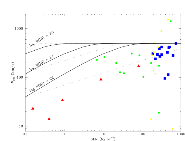
Figure 10: Terminal velocity of interstellar gas clouds accelerated by a hot wind. For consistency with X-ray measurements, the hot wind velocity is taken as 500 km s^-1 , independent of galaxy mass; and the mass flux in the wind is assumed equal to the SFR. Solid lines illustrate a model where the clouds are launched at a radius of 200 pc. Dotted lines show the effect of increasing the size of the launch region with the square root of the SFR as suggested by Heckman et al. (2000). The results illustrate the critical SFR below which the hot wind momentum is insufficient to accelerate the clouds to the velocity of the hot wind.

where $v_{w}$ is the velocity of the hot wind streaming out through solid angle $\Omega$. The momentum injection rate is $\dot{p}_{w}=\dot{m}_{w}v_{w}=\Omega\rho_{w}r^{2}v_{w}^{2}$, which is about $5\times 10^{33}(SFR/1\mbox{$~{}{\rm M_{\odot}}$~{}yr${}^{-1}$})$ dyne in a starburst (Leitherer et al. 1999). The absorbing clouds must enter the hot wind at relatively low velocities because the absorption line profiles extend smoothly to the systemic velocity. Replacing the time derivative in Equation 5 with $vdv/dr$, ignoring the gravitational deceleration, and integrating outward from the sound speed of the cool clouds, i.e. $\sim 6$ km/s, yields terminal cloud velocities that increase with SFR as illustrated in Figure 10. Up until the point where the clouds are moving with the hot wind, these solutions are well approximated by taking $v_{w}-v_{c}\approx v_{w}$ in Equation 5 giving terminal velocity

$$v_{term}=\left(\frac{3\dot{p}_{w}}{2\Omega\rho_{c}R_{0}^{2}}\right)^{1/2}=\left(\frac{3\rho_{w}(R_{0})}{2\rho_{c}}\right)^{1/2}v_{w}$$ (6)

for clouds of density $\rho_{c}$ launched from radius $R_{0}$ (e.g. Murray et al. 2004, Appendix A). Substituting $N_{c}=\rho_{c}\mu^{-1}m_{p}^{-1}R_{c}$, the fiducial wind speed of 500 km s^-1 , $\dot{m}_{w}=\lambda\dot{M}_{*}$, and an arbitrary launch radius of 200 pc, the maximum cloud velocity can be written

$$\frac{v_{term}}{v_{w}}=\left(\frac{\lambda\dot{M}_{*}}{0.24~{}{\rm M_{\odot}~{}yr}^{-1}}\right)^{0.5}\times$$

$$\left(\frac{10^{20}{\rm cm~{}}^{-2}}{N_{H}}\frac{200~{}{\rm pc}}{R_{0}}\frac{500{\rm~{}km~{}s}^{-1}}{v_{w}}\frac{\pi}{\Omega}\right)^{0.5},$$ (7)

where $\lambda\sim 1$ and $\mu$ was taken to be 1.4. This approximation indicates the critical SFR required to accelerate a cool gas column of $N_{H}\sim 10^{20},10^{21},{\rm~{}and~{}},10^{22}$ cm^-2 to 500 km s^-1  is 0.24$~{}{\rm M_{\odot}}$ yr^-1, 2.4$~{}{\rm M_{\odot}}$ yr^-1, and 24$~{}{\rm M_{\odot}}$ yr^-1, respectively. Taking proper account of the relative cloud – wind velocity in Figure 10 shows somewhat higher SFR’s, $\dot{M}_{*}\sim 0.7,7,70$$~{}{\rm M_{\odot}}$ yr^-1, are required to actually flow with the wind. Inspection of Figure 10 indicates that any combination of launch radius and column density satisfying $(\mu N/10^{22}{\rm~{}cm}^{-2})(R_{0}/200{\rm~{}pc})\sim 1$ is a good description of the upper envelope of the outflow velocities for all but a few extremely luminous ULIGs. The implied rate of momentum injection, $\dot{p_{w}}=2/3\Omega\mu m_{p}N_{H}R_{0}v_{\infty}^{2}$ or

$$\dot{p_{w}}=8.0\times 10^{34}{\rm~{}dyne~{}}(\Omega/\pi)N_{22}R_{0,200}v^{2}_{\infty,500},$$ (8)

which, for any solid angle $\Omega$, is easily supplied by a SFR of 70$~{}{\rm M_{\odot}}$ yr^-1 since $\dot{p}_{*}=3.5\times 10^{35}$ dyne. Supernova-driven winds can, it turns out, describe the observed increase in Na I velocities from ${\rm SFR}~{}0.1$ to roughly 100$~{}{\rm M_{\odot}}$ yr^-1 and still be consistent with X-ray temperatures that are independent of galaxy mass.

It should be emphasized that the terminal cloud velocity is sensitive to the launch radius because most of the cloud acceleration happens at small radii where the ram pressure is largest. If the size of the starburst region, and consequently the launch region for the wind, grows as the SFR increases, then the terminal velocities rise more slowly than $SFR^{0.5}$. Figure 10 illustrates the constant surface brightness case previously suggested by Heckman et al. (2000), which implies $v_{term}\propto{\rm~{}SFR}^{1/4}$. This scaling for the size of the launch region fails to reproduce the steep slope of the outflow velocity envelope from dwarf starburst to LIG luminosities.

It is not obvious that the hot wind would naturally tune the terminal cloud velocities to match the rotation speed of the parent galaxy as suggested by Figure 8. This correlation implicitly requires $\dot{p}_{w}$ to be connected to the halo mass, presumably via the SFR. Some simple recipes are explored here. Using an isothermal halo with velocity dispersion $\sigma$ to model the halo mass distribution, $M(r)=2G^{-1}\sigma^{2}r$, Equation 5 becomes

$$\frac{dv_{c}}{dr}=\frac{-2\sigma^{2}}{v_{c}r}+\frac{3\dot{p}_{w}}{4N_{H}\mu m_{h}\Omega}\left(1-\frac{v_{c}}{v_{w}}\right)\frac{1}{v_{c}r^{2}},$$ (9)

which is easily solved for $v(r)$ when $v_{c}<<v_{w}$. In order for the clouds to move out a significant distance, the solution suggests the characteristic flow velocity $v_{char}=\sqrt{3\dot{m_{w}}v_{w}/(2\Omega N_{H}R_{0}m_{p}\mu)}$ must exceed $2\sigma$ (e.g. Murray, Quataert, & Thompson 2004). For purposes of illustration, suppose the star formation rate scales as $SFR\propto f_{g}M_{tot}/t_{dyn}\propto\sigma^{3}$, where $f_{g}M_{tot}$ is the gas mass of the galaxy. This scaling is plausible since the mass of a galaxy increases as $\sigma^{3}$ and the dynamical timescale of a disk, $R_{d}/V$, is independent of mass (Mo, Mao, White 1998). Normalizing to the stellar velocity dispersions in IRAS23365+3604, IRAS20087-0308, and IRAS17208-0014 (Genzel et al. 2001) gives $SFR\approx 500\mbox{$~{}{\rm M_{\odot}}$~{}yr${}^{-1}$}(\sigma/210\mbox{~{}km~{}s${}^{-1}$})^{3}$. Using this relation and integrating Equation 9 from low initial velocity at $R_{0}=200$ pc, clouds accelerate to the velocities shown in the top panel of Figure 11 before gravity slows them down. Choosing $(N_{H}/10^{22}$ cm${}^{-2})(R_{0}/200{\rm~{}pc})\approx 1$ again provides the best normalization to the data. With this $SFR\propto\sigma^{3}$ recipe, the cloud velocities rise steeply with the rotation speed because star formation is greatly suppressed in the low mass galaxies. Scaling the SFR as $\sigma^{2}$ or $\sigma$ produces a much more gradual rise in outflow speed with rotation speed, and these models are not consistent with the data.

This exercise demonstrates that ram pressure from a supernova-heated wind accelerates cool gas to a maximum velocity determined by the temperature of the momentum-carrying component of the hot wind. Outflow velocities measured for the 2 Jy sample of ULIGs are consistent with a maximum wind speed near $v~{}500$ km s^-1 , but more measurements will be required to confirm or refute this suggestion. Indeed, in Figure 10, four galaxies from the Rupke et al. and Heckman et al. samples present outflows significantly faster than this fiducial maximum. Several of the 2 Jy ULIGs also show absorption, albeit far from line center, at velocities in excess of 500 km s^-1 . Failure of the outflow measurements to define an asymptotic velocity might reveal (1) the presence of a hotter wind component or (2) an acceleration mechanism other than supernova. The awkwardness of the supernova-driven wind model for explaining the terminal velocity – rotation speed correlation motivates some consideration of alternative acceleration mechanisms.

5.2 Radiatively-Driven Winds

Stellar wind velocities exhibit a scaling similar to that found here for galactic winds. The terminal wind velocities from central stars of planetary nebulae are typically 4.4 times the escape velocity at the stellar surface (Lamers & Cassinelli 1999). Is this remarkable coincidence an indication that the underlying wind physics is similar? The correlation seems natural in stellar winds. The wind is accelerated by radiation pressure on dust grains, and the maximum surface luminosity is limited by the requirement of hydrostatic equilibrium. In galaxies, the SFR determines the momentum of the hot wind, but the relation between galaxy mass and SFR is complicated by variable quantities such as the gas fraction and the star formation efficiency. Radiatively-driven winds on a galactic scale have an appealing property, namely that the galactic luminosity cannot increase much beyond an effective Eddington-like luminosity.

The radiative force exerted on the cool gas from dust absorption usually dominates over that from photoelectric absorption by gas. For the radiatively-driven wind concept to be viable for galaxies, the dust grains need to survive in the outflow and pull the gas along. Dust grains in the interstellar medium are charged and typically couple electrostatically to the gas (Draine 2003). Sputtering following the passage of a shock destroys grains, but calculations suggest significant amounts of dust survive in radio galaxies (De Young 1998; Villar-Martin et al. 2001). Several types of observations strongly suggest that starburst winds are indeed dusty. First, the Na I line is a resonance line, so the absorbed photons are re-emitted in random directions. The absence of Na I emission in the ULIG spectra presented in this paper suggests the re-emitted photons are absorbed by dust (and converted to heat) before they can escape the galaxy. Second, the thermal emission from cold dust in starburst galaxies has a significantly larger scale-height than the stars indicating dust is lofted above the region where it forms (Engelbract et al. 2004, NGC 55; Popescu et al. 2004, NGC 891). Third, extended red emission, a broad emission band seen in many dusty astrophysical objects, has been detected in the halo of the superwind galaxy M82 (Perrin, Darbon, Sivan 1995; Gordon, Witt, & Friedmann 1998). Furthermore, recent GALEX imaging of M82 show ultraviolet halo emission significantly brighter than expected from the nebular continuum, which likely indicates the light is scattered by small grains (Chris Martin, pvt comm). The dynamical implications of dust in these winds needs to be considered.

Little ultraviolet radiation emerges from ULIGs implying these galaxies are optically thick to much of the intrinsic starburst luminosity. The radiative force on the gas clouds is $F_{rad}=M_{c}c^{-1}\int\kappa_{\nu}F_{\nu}d\nu$, where the absorption opacity of the dust and gas mixture, $\kappa$, drops from 600 cm${}^{2}~{}{\rm g}^{-1}$ near 1000 Å to 100 cm${}^{2}~{}{\rm g}^{-1}$ in the U band (Li & Draine 2001). In the optically thick limit, the radiation force reaches $L/c$ and balances the gravitational force on the cool interstellar gas when the luminosity reaches $L_{crit,ED}=4G^{-1}cf_{g}\sigma^{4}$. For a fiducial halo velocity dispersion of 150 km s^-1 , the critical luminosity required to radiatively accelerate most of the cool interstellar gas is then

$$L_{crit,ED}=2.4\times 10^{12}{~{}\rm L_{\odot}}\left(\frac{\sigma}{150{\rm~{}km/s~{}}}\right)^{4}\left(\frac{f_{g}}{0.1}\right).$$ (10)

The fraction of the galactic mass in the cool wind, $f_{g}$, will be less than 0.1, so the ULIG luminosities appear high enough to radiatively accelerate significant amounts of cool gas and dust. Assuming a starburst duration of 100 Myr (Leitherer 1999) and a Salpeter ($\alpha=2.35$) initial mass function from 0.1 to 100${\rm~{}M_{\odot}}$, the corresponding star formation rate where radiation pressure becomes important for wind acceleration is

$$\dot{SFR}_{crit}\sim 400\mbox{$~{}{\rm M_{\odot}}$~{}yr${}^{-1}$}\ \left(\frac{\sigma}{150{\rm~{}km~{}s}^{-1}}\right)^{4}\frac{f_{g}}{0.1}.$$ (11)

Any additional (besides supernova) acceleration mechanism should predict the highest outflow speeds and/or explain why most outflows are tuned to the rotation (or escape) speed. The latter is clear. Once the starburst luminosity exceeds $L_{crit,ED}$, the cloud is accelerated from rest at $R_{0}$ to $v(r)=2\sigma\sqrt{(L/L_{crit,ED}-1)ln(r/R_{0})}$ (e.g. Murray, Quartaert, and Thompson 2004). The weak radial dependence indicates the terminal cloud velocity depends mainly on the ratio $L/L_{crit,ED}$. Figure 11 (bottom panel) demonstrates that $L/L_{crit,ED}\sim 2$ provides an excellent description of the correlation between outflow velocities and rotation speed.

The outflow speeds exceeding 500 km s^-1  could have several explanations. If radiation pressure is the dominant acceleration mechanism, then starbursts are not the source of luminosity because extrapolation of the velocities in Figure 11 to 1500 km s^-1  implies rotation speeds larger than galaxies. AGN would have to supply the radiative acceleration. Ram-pressure could also accelerate cool gas to these high velocities if the clouds are launched from small radii associated with AGN rather than starburst radii. Inspection of the starburst spectra with outflows faster than 500 km s^-1 indicates IRAS-FSC05024-1941 (1538 km s^-1 , Rupke et al. 2002) has cool infrared colors but is optically identified as a Seyfert 2; IRAS11119+3257 (1410  km s^-1 , Heckman et al. 2000) has warm infrared color. It therefore seems quite likely that both these objects have active nuclei, and one can speculate that AGN are responsible for the abnormally high velocities. A much larger database will clearly be required to determine the relative roles of AGN and starbursts in driving winds. Among the the 2 Jy CO-subsample, however, only IRAS11506+1331 shows Seyfert 2 activity, and it does not present an unusually fast wind.

6 Conclusions

Doppler shifts measured from interstellar absorption lines in starburst spectra reveal cool gasesous outflows. The fraction of starbursts presenting outflows increases with starburst luminosity reflecting either the brief duty cycle of the ultraluminous phase or the large solid angle subtended by these winds. The cool outflow does not entirely cover the optical nucleus indicating clouds or shells are a better description than a continuous fluid. The covering fraction approaches unity in the galaxies with the strongest winds (i.e. largest equivalent width), and these merging systems are usually found to be near perigalactic passage. More widely separated systems and single-nuclei systems generally have lower covering factors and line strengths. These results lead to the conclusions that (1) much of the mass loading occurs very near perigalactic passage and (2) the mass loading is gradually shut down as the nuclei finish merging. The mass entrainment rate of cold clouds is quite large, possibly comparable to the SFR, and is discussed in more detail in Paper II.

Galaxies with higher SFRs accelerate the absorbing clouds to higher velocities. Projection effects introduce a large range in measured velocities at a given SFR, but the maximum outflow velocity rises roughly as $SFR^{1/3}$. This trend challenges the hypothesis that the clouds are accelerated by the hot winds, whose emission-measure weighted temperatures appear to vary little with circular velocity. The simplest explanation is that the clouds in the ultraluminous starbursts reach terminal velocities comparable to the velocity of the hot winds, and that the low Na I wind velocities in dwarf starbursts reflect a shortage of momentum in dwarf starburst winds.

However, in order for momentum-driven winds to explain the intriguing similarity between the terminal cloud velocity and the galactic escape velocity, the rate of momentum injection must be tightly correlated with the depth of the gravitational potential. Radiatively-driven winds naturally provide this connection via a galactic equivalent to the stellar Eddington luminosity, while rather ad hoc recipes between the SFR and dark halo mass must be cooked up for supernova-driven winds. A highly simplified description of how dusty clouds would be accelerated by the starburst continuum luminosity demonstrates that ULIG luminosities are sufficient to accelerate significant columns of cool gas to the observed Na I velocities.

These results draw attention to the importance of feedback in very massive galaxies. Preliminary estimates of the mass loss rates suggest a significant fraction of the ISM participates in the cool outflows. This result is surprising in the context of energy-driven winds because a large fraction of the supernova energy is expected to be radiated away in the dense molecular ISM of an ULIG. Much as supernova feedback is most effective in dwarf galaxies where hot gas can escape from the halo, radiative feedback is naturally strongest in the densest, most luminous galaxies. Hence, radiative feedback may help explain the differences between the shape of the halo mass function and the galaxy luminosity function at the high-mass end. The dynamical properties of the stars in ULIGs do appear to be consistent with those of field ellipticals (Genzel et al. 2001), so it is also appealing to associate the winds seen in ULIGs with the event that shuts the star formation down quickly enough to create high ratios of alpha elements to iron in elliptical galaxies.

Filling in Figure 10 and Figure 11 with more observations will help clarify some of these isssues. Also, since radiatively-driven winds do not require a hot phase, X-ray observations of these ULIGs may distinguish acceleration mechanisms. Spitzer and GALEX observations will be instrumental for constraining the amount of extraplanar dust in starbursts and its composition. A few of the most luminous objects present velocities too high to explain with starburst winds, so it will be possible to explore the nature of outflows in warm ULIGs during the SB/AGN transition. More detailed dynamical modeling of the survivability and fate of the cool clouds as well as a more realistic treatment of radiation pressure will allow a more detailed comparison to the data (e.g. line widths, spatial gradients, etc.) and thereby a more stringent test of the ideas presented here.

Table 1: Sample of Galaxies

Object	z	$L_{FIR}$	$L_{IR}$	SFR
	(CO)	(${~{}\rm L_{\odot}}$)	(${~{}\rm L_{\odot}}$)	($~{}{\rm M_{\odot}}$ yr-1)
IRAS00153+5454	0.1120	11.94	12.27	320
IRAS00188-0856	0.1285	12.18	12.41	450
IRAS00262+4251	0.09724	11.90	12.16	250
IRAS03158+4227	0.1344	12.39	12.64	750
IRAS03521+0028	0.1519	12.33	12.57	640
IRAS08030+5243	0.08350	11.82	12.05	190
IRAS10494+4424	0.09231	11.99	12.23	290
IRAS10565+2448	0.04311	11.81	12.05	190
IRAS11506+1331	0.1273	12.11	12.35	390
IRAS15245+1019	0.0757	11.81	12.10	220
IRAS16090-0139	0.1336	12.34	12.57	630
IRAS16487+5447	0.1036	11.98	12.29	330
IRAS17208-0014	0.04282	12.23	12.45	490
IRAS18368+3549	0.1162	12.03	12.27	320
IRAS19297-0406	0.08573	12.21	12.44	470
IRAS19458+0944	0.1000	12.15	12.39	420
IRAS20087-0308	0.1057	12.23	12.47	510
IRAS23365+3604	0.06448	11.96	12.20	280

Table Notes: (1) Object name. (2) Redshifts from Solomon et al. (1997) except IRAS 00153+5454, IRAS 15245+1019, and IRAS 16487+5447 which are from Dr. Aaron Evans (pvt. comm.). Velocities have errors of $\pm cz\approx 20$ km s^-1 . (3) The far-infrared luminosity computed from $L_{FIR}=3.86\times 10^{5}\mbox{${~{}\rm L_{\odot}}$}d_{L}^{2}(2.58F_{\nu}(60um)+f_{\nu}(100um))$, where the flux density is in Janskys and the luminosity distance (h=0.7, $\Omega_{0}=0.3$ and $\Omega_{\Lambda}=0.7$) is in Mpc. (4) The estimated 8 - 1000 um luminosity $L_{\rm IR}$ (h=0.7, $\Omega_{0}=0.3$ and $\Omega_{\Lambda}=0.7$). The IRAS 12um fluxes for the galaxies in this sample are upper limits, so the median flux ratios of bright ULIGs with IRAS detections in all four bands were used to estimate $L_{\rm IR}$ as described in Murphy et al. (1996). (5) The star formation rate estimated from $SFR=L_{\rm IR}/5.8\times 10^{9}$ ${~{}\rm L_{\odot}}$(Kennicutt 1989), where the luminosity is the estimated bolometric luminosity $L_{\rm IR}$. This relation uses the continuous star formation model of Leitherer et al. (1999) and a Salpeter initial mass function from 0.1 to 100 ${\rm~{}M_{\odot}}$.

Table 2: Properties of Na I Absorption

Object	$W({\rm NaD})$	$f_{*}$	$v_{max}$	$C_{f}$	$\Delta l$
	(Å)	(Å)	( km s-1 )		(${\rm h}_{70}^{-1}$ kpc)
IRAS00153+5454	$4.1\pm 0.5$	0.15	-715	0.14	3.8 (7$\farcs$3)
IRAS00188-0856	$7.5\pm 0.6$	0.09	-751	0.19	4.6 (1$\farcs$9)
IRAS00262+4251	$1.0\pm 0.3$	0.33	-580	0.11	6.9 (3$\farcs$8)
IRAS03158+4227	$5.1\pm 0.4$	0.052	-1047	0.25	6.2 (2$\farcs$6)
IRAS03521+0028	$5.1\pm 0.4$	0.1	-350	0.63	5.0 (1$\farcs$9)
IRAS08030+5243	$7.4\pm 1.0$	0.063	-311	0.26	$\buildrel{\scriptstyle>}\over{\scriptstyle\sim}$ 8.2 (5$\farcs$2)
IRAS10494+4424	$5.6\pm 0.1$	0.024	-560	0.15	$\buildrel{\scriptstyle>}\over{\scriptstyle\sim}$ 12.0 (7$\farcs$0)
IRAS10565+2448	$10.4\pm 0.1$	0.03	-620	0.42	$\buildrel{\scriptstyle>}\over{\scriptstyle\sim}$ 11.4 (13$\farcs$4)
IRAS11506+1331	$3.88\pm 0.2$	0.10	-435	0.28	4.53 (1$\farcs$9)
IRAS15245+1019	$8.5\pm 0.1$	0.05	-559	0.67	4.2 (12$\farcs$4)
IRAS16090-0139	$3.32\pm 0.06$	0.083	-543	0.11	7.6 (3$\farcs$2)
IRAS16487+5447	$<0.5$	$>0.46$	$\cdots$	$\cdots$	2.71 (5$\farcs$7)
IRAS17208-0014	$9.4\pm 0.1$	0.06	-691	0.52	$\buildrel{\scriptstyle>}\over{\scriptstyle\sim}$ 7.3 (8$\farcs$6)
IRAS18368+3549	$9.0\pm 0.3$	0.04	-768	0.25	10.3 (4$\farcs$8)
IRAS19297-0406	$3.7\pm 0.2$	0.12	-697	0.22	4.8 (2$\farcs$9)
IRAS19458+0944	$4.0$	$\cdots$	$\cdots$	$\cdots$
IRAS20087-0308	$9.0\pm 1.5$	0.074	-1082	0.26	12.2 (6$\farcs$3)
IRAS23365+3604	$4.5\pm 0.4$	0.12	-651	0.16	5.9 (4$\farcs$7)

Table Notes –

(1) Object name.

(2) Total measured NaD absorption equivalent width (observed frame).

(3) Fraction of total NaD equivalent width from a stellar component predicted from measured Mgb equivalent width and the relation $W(\mbox{Na~{}I})=1/3W(Mg~{}I)$ described in the text.

(4) Terminal velocity measured from the intersection of the bluest part of the absorption line with the continuum.

(5) Fraction of continuum source covered by absorbing clouds where $C_{f}\equiv 1-I(\lambda 5890)$.

Table 3: Fitted Na I Absorption (Optically Thick)

Object	$W_{Dop}$	$v_{B}$	$\Delta v_{B}$	$\Delta v_{sys}$	$D_{B}$	$N_{NaI}$
	(Å)	( km s-1 )	( km s-1 )	( km s-1 )		($10^{12}$ cm-2)
IRAS00153+5454	3.7	$-292\pm 15$	$452\pm 40$	$554\pm 219$	$\lower 2.0pt\hbox{$\buildrel{\scriptstyle<}\over{\scriptstyle\sim}$}\ 1.06\pm 0.06$	$436_{-392}^{+\inf}$
IRAS00188-0856	4.42	$-328\pm 30$	$520\pm 20$	$260\pm 11$	$1.07\pm 0.09$	$310^{+\inf}_{-210}$
IRAS00262+4251	0.94	$-293\pm 20$	$296\pm 20$	$500\pm 150$	$1.7\pm 0.4$	$1.53_{-0.25}^{+0.94}$
IRAS03158+4227	4.43	$-499\pm 25$	$405\pm 35$	$312\pm 90$	$1.21\pm 0.15$	$25_{-8}^{+12}$
IRAS03521+0028	5.0	$-77\pm 12$	$175\pm 31$	$636\pm 360$	$1.42\pm 0.46$	$1.67_{-5.4}^{270}$
IRAS08030+5243	4.02	$+267\pm 2$	$158\pm 4$	$350\pm 30$	$1.16\pm 0.05$	$29.8_{-0.85}^{+4.4}$
IRAS10494+4424	2.85	$-270\pm 23$	$315\pm 35$	$237\pm 7$	$1.07\pm 0.18$	$174^{+\inf}_{-160}$
IRAS10565+2448a	7.80	$-307\pm 16$	$307\pm 16$	$278\pm 107$	$\lower 2.0pt\hbox{$\buildrel{\scriptstyle<}\over{\scriptstyle\sim}$}\ 1.10$	$\lower 2.0pt\hbox{$\buildrel{\scriptstyle>}\over{\scriptstyle\sim}$}\ 160$
IRAS10565+2448b	5.1	$-87\pm 2$	$188\pm 10$	”	$1.33\pm 0.18$	$19.6_{-4.3}^{20.6}$
IRAS11506+1331	3.3	$-96\pm 6$	$242\pm 10$	$222\pm 150$	$1.10\pm 0.07$	$59.8_{-37.4}^{+\inf}$
IRAS15245+1019	8.9	$-240\pm 4$	$301\pm 6$	$347\pm 108$	$1.24\pm 0.03$	$43.1_{-3.6}^{+5.2}$
IRAS16090-0139	1.31	$-282\pm 23$	$296\pm 25$	$354\pm 22$	$1.96\pm 0.28$	$2.1_{-0.2}^{+4.9}$
IRAS16487+5447	$\cdots$	$\cdots$	$\cdots$	$\cdots$	$\cdots$	$\cdots$
IRAS17208-0014	6.91	$-409\pm 3$	$292\pm 4$	$254\pm 6$	$1.06\pm 0.02$	$883_{-612}^{+\inf}$
IRAS18368+3549a	4.64	$-420\pm 35$	$371\pm 49$	$364\pm 134$	$1.06\pm 0.28$	$567_{-547}^{+\inf}$
IRAS18368+3549b	4.89	$-143\pm 4$	$213\pm 12$	”	$1.24\pm 0.24$	$22.6_{-8.1}^{+\inf}$
IRAS19297-0406	3.84	$-114\pm 16$	$377\pm 26$	$313\pm 60$	$1.46\pm 0.18$	$11_{-1.9}^{+5.4}$
IRAS19458+0944	$\cdots$	$\cdots$	$\cdots$	$\cdots$	$\cdots$	$\cdots$
IRAS20087-0308	4.3	$-420\pm 50$	$628\pm 57$	$478\pm 113$	$1.87\pm 0.36$	$9.25_{-0.44}^{+2.95}$
IRAS23365+3604	1.80	$-389\pm 72$	$308\pm 85$	$610\pm 195$	$1.26\pm 0.79$	$8.27_{-6.04}^{+\inf}$

Table Notes –

(1) Object name. Spectral model is the sum of a Na I doublet at the systemic velocity and a doublet, the dynamic component, for which the velocity is fitted. The doublet ratio, $D\equiv W(\lambda 5890)/W(\lambda 5896)$, of the systemic component was held at $D=1.06$ – equivalent to an $\lambda 5890$ optical depth of 142. The doublet ratio of the dynamic component was fitted.

(2) Equivalent width of fitted Doppler-shifted component.

(3) Fitted velocity of Doppler shifted interstellar component.

(4) FWHM of fitted Doppler shifted interstellar component.

(5) FWHM of the component at the systemic velocity. Parentheses indicate an assumed, rather than fitted, value.

(6) Fitted doublet ratio, $D\equiv W(5895)/W(5889)$ of Doppler shifted interstellar component.

(7) Constraints on column density from curve of growth analysis and doublet ratio from column 3.

Table 4: Fitted Na I Absorption (Optically Thin)

Object	$W_{Dop}$	$v_{B}$	$\Delta v_{B}$	$\Delta v_{sys}$	$N_{NaI}$
	(Å)	( km s-1 )	( km s-1 )	( km s-1 )	($10^{12}$ cm-2)
IRAS00153+5454	3.2	$-289\pm 42$	$499\pm 48$	$293\pm 42$	$9.94\pm 0.67$
IRAS00188-0856	4.3	$-340\pm 28$	$567\pm 36$	$332\pm 15$	$13.1\pm 0.6$
IRAS00262+4251	0.5	$-406\pm 20$	$232\pm 21$	$493\pm 46$	$1.5\pm 0.6$
IRAS03158+4227	5.3	$-469\pm 11$	$466\pm 29$	$340\pm 83$	$15.67\pm 0.33$
IRAS03521+0028	3.8	$-94\pm 15$	$152\pm 46$	$530\pm 200$	$13.1\pm 4.3$
IRAS08030+5243	4.2	$+268\pm 5$	$166\pm 16$	$536\pm 397$	$13.1\pm 1.1$
IRAS10494+4424	1.2	$-380\pm 57$	$356\pm 80$	$318\pm 15$	$3.84\pm 0.65$
IRAS10565+2448a	7.7	$-252\pm 22$	$469\pm 24$	$283\pm 29$	$25.14\pm 0.11$
IRAS10565+2448b	3.9	$-88\pm 3$	$156\pm 5$	”	$12.94\pm 0.04$
IRAS11506+1331	3.4	$-58\pm 2$	$338\pm 27$	$305\pm 90$	$10.37\pm 0.02$
IRAS15245+1019	7.4	$-243\pm 6$	$296\pm 8$	$307\pm 20$	$23.31\pm 0.04$
IRAS16090-0139	0.7	$-325\pm 40$	$281\pm 37$	$479\pm 29$	$2.16\pm 0.36$
IRAS16487+5447	$\cdots$	$\cdots$	$\cdots$	$\cdots$	$\cdots$
IRAS17208-0014	7.4	$-359\pm 15$	$462\pm 38$	$253\pm 13$	$21.18\pm 0.08$
IRAS18368+3549a	5.4	$-341\pm 56$	$469\pm 66$	$354\pm 37$	$16.59\pm 0.17$
IRAS18368+3549b	3.0	$-140\pm 7$	$168\pm 19$	”	$9.46\pm 0.10$
IRAS19297-0406	3.6	$-413\pm 13$	$370\pm 22$	$286\pm 36$	$11.3\pm 0.6$
IRAS19458+0944	$\cdots$	$\cdots$	$\cdots$	$\cdots$	$\cdots$
IRAS20087-0308	4.6	$-421\pm 50$	$631\pm 75$	$525\pm 703$	$14.3\pm 0.8$
IRAS23365+3604	1.3	$-384\pm 96$	$302\pm 22$	$660\pm 179$	$4.3\pm 1.5$

Table Notes –

(1) Object name. Spectral model is the sum of a Na I doublet at the systemic velocity and a doublet, the dynamic component, for which the velocity is fitted. The doublet ratio was fixed at the optically thin limit.

(2) Equivalent width of fitted Doppler-shifted component.

(3) Fitted velocity of Doppler shifted interstellar component.

(4) FWHM of fitted Doppler shifted interstellar component.

(5) FWHM of the component at the systemic velocity. Parentheses indicate an assumed, rather than fitted, value.

(6) Column density of Na I.

Figure 1: (b) The ESI spectra around the Na I $\lambda 5890,96$ doublet. The emission line is He I $\lambda 5876$. No Na I absorption was detected in IRAS16487+5447 and IRAS19458+0944. The dotted line shows a doublet at the systemic velocity, which was determined from observations of the molecular gas. The doublet ratio of the systemic component is fixed at $EW(5890)/EW(5896)=1.06$ here. The Doppler shift and doublet ratio of the dynamic component, shown by the thin solid line, were fitted. The heavy solid line shows the sum of the dynamic component, systemic component, and the He I emission line. All but one galaxy presents a highly blueshifted dynamic component.

Figure 2: Measured Na D absorption equivalent width versus measured Mg I absorption equivalent width in ULIGs. The solid line is a fit to stellar spectra (see §3.1 of text), and the dotted line illustrates typical values in elliptical galaxies (Bica et al. 1991).

Figure 3: The K I 7664.9 profile for the five galaxies with the strongest interstellar absorption. The weaker member of the doublet is at $+1327$ km s^-1  (not shown). The Na I doublet, arbitrarily scaled, is overlaid. The profiles deviate, as they must, redward of the systemic velocity where the Na I 5890 appears. The spikes in the K I spectra are residuals from the subtraction of bright night sky lines and should be ignored. The K I 7664.9 absorption profile is generally similar in shape to the Na I 5889 profile but has poor signal-to-noise ratio.

Figure 5: (Left ) The Na I equivalent width shows no correlation with the velocity width of the line. (Right) Cloud covering factor versus Na I equivalent width in the dynamic component. The sightlines with the highest covering factors present the strongest absorption lines.

Figure 9: Wind strength at progressive stages of the merger. The absorption lines are strongest when the merging galaxies are near perigalacticon. They become weaker around apogalacticon and again following the merger of the nuclei.

References

- (1)
- (2) Aguirre, A. et al. 2001, ApJ, 561, 521
- (3)
- (4) Andrews, S. Meyer, D. M. & Lauroesch, J. T. 2001, ApJ, 552, L73
- (5)
- (6) Barkana, R., & Loeb, A. 1999, ApJ, 523, 54
- (7)
- (8) Benson, A. J. et al. 2003, ApJ, 599, 38
- (9)
- (10) Bernardi, M. et al. 2003, AJ, 125, 1849
- (11)
- (12) Bica, E. et al. 1991, AJ, 102, 1702
- (13)
- (14) Blanton, M. R. et al. 2003, ApJ, 594, 186
- (15)
- (16) Bond, N. A., Churchill, C. W., Charlton, J. C., & Vogt, S. S. 2001, ApJ, 562, 641
- (17)
- (18) Borne, K. D., Bushouse, H., Lucas, R. A., & Colina, L. 2000, ApJ, 529, L77, 2000.
- (19)
- (20) Chevalier, R. A. & Clegg, A. W. 1985, Nature, 317, 44
- (21)
- (22) Dale, D. A. et al. 1999, AJ, 118, 1489
- (23)
- (24) Dekel, A. & Silk, J. 1986, ApJ, 303, 39
- (25)
- (26) Dekel, A., & Woo, J. 2003, MNRAS, 344, 1131
- (27)
- (28) De Young, D. S. 1998, ApJ, 507, 161
- (29)
- (30) Draine, B. T. 2003, Astrophysics of Dust in Cold Clouds, Saas-Fee Advanced Course 32, Berlin: Springer-Verlag, in press
- (31)
- (32) Engelbracht, C. W. et al. 2004, ApJS, in press
- (33)
- (34) Gao, Y. & Solomon, P. M. 1999, ApJ, 512, 99
- (35)
- (36) Garnett, D. R. 2002, ApJ, 581, 1019
- (37)
- (38) Genzel, R. et al. 2001, ApJ, 563, 527
- (39)
- (40) Gordon, K. D., Witt, A. N., & Friedmann, B. C. 1998, ApJ, 498, 522
- (41)
- (42) Heckman, T., Armus, L., & Miley, G. K. 1990, ApJS, 74, 833
- (43)
- (44) Heckman, T., Lehnert, M. D., Strickland D. K., & Lee, A. 2000, ApJS, 129, 493
- (45)
- (46) Hibbard, J. E., Vacca, W. D., & Yun, M. S. 2000, AJ, 119, 1130
- (47)
- (48) Hunter, D. A., vanWoerden, H., & Gallagher, J. S. 1999, AJ, 118, 2184
- (49)
- (50) Ivison, R. J. et al. 2000, MNRAS, 315, 209
- (51)
- (52) Kauffmann, G. et al. 2003a, MNRAS, 341, 33
- (53)
- (54) Kauffmann, G. et al. 2003b, MNRAS, 341, 54
- (55)
- (56) Kennicutt, R. C. Jr. 1989, ApJ, 344, 685
- (57)
- (58) Lamers & Cassinelli 1999, Introduction to Stellar Winds, Cambridge Univ. Press
- (59)
- (60) Larson, R. 1974, 169, 229
- (61)
- (62) Leitherer, C. et al. 1999, ApJS, 123, 3
- (63)
- (64) Mac Low, M.-M. & Ferrara, A. 1999, ApJ, 513, 142
- (65)
- (66) Martin, C. L. 1999, ApJ, 513, 156
- (67)
- (68) Martin, C. L. 2004, in Origin and Evolution of the Elements, ed. A. McWilliam & M. Rauch, (Cambridge: Cambridge Uhiv. Press)
- (69)
- (70) Martin, C. L., Kobulnicky, H. A., & Heckman, T. M. 2002, ApJ, 574, 663
- (71)
- (72) Meurer, G. et al. 1997, AJ, 114, 54
- (73)
- (74) Mo, H. J., Mao, S., & White, S. D. M. 1998, MNRAS, 295, 319
- (75)
- (76) Murphy, T. W. et al. 1996, AJ, 111, 1025.
- (77)
- (78) Murphy, T. W. et al. 2001, ApJ, 55, 201
- (79)
- (80) Murray, N. Quataert, E., & Thompson, T. A. 2004, ApJ, submitted
- (81)
- (82) Norman, C., Bowen, D. V., Heckman, T., Blades, C., & Danly, L. 1996, ApJ472, 73
- (83)
- (84) Perrin, J.-M., Darbon, S., & Sivan, J.-P. 1995, A&A, 304, L21
- (85)
- (86) Pettini, M. et al. 2001, ApJ, 554, 981
- (87)
- (88) Pettini, M. et al. 2002 ApJ, 569, 742
- (89)
- (90) Popescu, C. C. et al. 2004, A&A, 414, 45
- (91)
- (92) Rupke, D. S., Veilleux, S., & Sanders, D. B. 2002, ApJ, 570, 588
- (93)
- (94) Sanders, D. B., Scoville, N. Z., Sargent, A. I., & Soifer, B. T. 1988a, ApJ, 324, L55
- (95)
- (96) Sanders, D. et al. 1988b, ApJ, 325, 74
- (97)
- (98) Sanders, D. et al. 2003, AJ, 126, 1607
- (99)
- (100) Scannapieco, E., Thacker, R., & Davis, M. 2001, ApJ, 557, 605
- (101)
- (102) Scannapieco, E. & Oh, P. 2004, ApJ, in press
- (103)
- (104) Scoville, N. Z. et al. 2000, AJ, 119, 991
- (105)
- (106) Scoville, N. Z. et al. 2001, AJ, 122, 3017
- (107)
- (108) Scoville, N. Z. 2003, Journal of the Korean Astronomical Society, 36, 167
- (109)
- (110) Schwartz, C. & Martin, C. L. 2004, ApJ, 610, 201
- (111)
- (112) Shapley, A. E. et al. 2003, ApJ, 588, 65
- (113)
- (114) Silich, S., & Tenorio-Tagle, G. 2001, ApJ, 552, 91
- (115)
- (116) Solomon, P. M., Downes, D., Radford, S.J.E, & Barrett, J. W. 1997, ApJ, 478, 144
- (117)
- (118) Somerville, R. & Primack, J. R. 1999, MNRAS, 310, 1087
- (119)
- (120) Spitzer, L. Jr. 1968, Diffuse Matter in Space, John Wiley & Sons, Inc., p. 84-85.
- (121)
- (122) Sprayberry et al. 1995, AJ, 109, 558
- (123)
- (124) Stil, J. M. & Israel, F. P. 2002, A&A, 392, 473
- (125)
- (126) Strauss, M. A. et al. 1992, ApJS, 83, 29.
- (127)
- (128) Strickland, D. K. & Stevens, I. R. 2000, MNRAS, 314, 511
- (129)
- (130) Strickland, D. K. et al. 2002, ApJ, 568, 689
- (131)
- (132) Suchkov, A. A. et al. 1994, ApJ, 430, 511
- (133)
- (134) Suchkov, A. A. et al. 1996, ApJ, 463, 528
- (135)
- (136) Tremonti, C. A. 2004, ApJ, in press
- (137)
- (138) Vader, J. P. 1987, ApJ, 317, 128
- (139)
- (140) Villar-Martin, M. et al. 2001, MNRAS, 328, 848
- (141)
- (142) Walter, F., Taylor, C. L., H.̇uttemeister, S., Scoville, N., & McIntyre, V. 2001, AJ, 121, 727
- (143)
- (144) Zwaan, M. A. et al. 1995, MNRAS, 273, L35
- (145)