Abstract

We discuss the expected properties of the first stellar generations in the Universe. We find that it is possible to discern truly primordial populations from the next generation of stars by measuring the metallicity of high-z star forming objects. The very low background of the future James Webb Space Telescope (JWST) will enable it to image and study first-light sources at very high redshifts, whereas its relatively small collecting area limits its capability in obtaining spectra of z$\sim$10–15 first-light sources to either the bright end of their luminosity function or to strongly lensed sources. With a suitable investment of observing time  JWST will be able to detect individual Population III supernovae, thus identifying the very first stars that formed in the Universe.

Detecting Primordial Stars

Detecting Primordial Stars

1 Introduction

One of the primary goals of modern cosmology is to answer the question: “When did galaxies begin to form in the early Universe and how did they form?” Theorists predict that the formation of galaxies is a gradual process in which progressively larger, virialized masses, composed mostly of dark matter, harbor star formation as time elapses. These dark-matter halos, which harbor stellar populations, then undergo a process of hierarchical merging and evolution to become the galaxies that make up the local Universe. In order to understand what are the earliest building blocks of galaxies like our own, one must detect and identify “first light” sources, i.e, the emission from the first objects in the Universe to undergo star formation.

The standard picture is that at zero metallicity the Jeans mass in star forming clouds is much higher than it is in the local Universe, and, therefore, the formation of massive stars, say, 100 M_⊙ or higher, is highly favored. The spectral distributions of these massive stars are characterized by effective temperatures on the Main Sequence (MS) around $10^{5}$ K (e.g., Tumlinson & Shull 2000, Bromm et al. 2001, Marigo et al. 2001). Due to their temperatures these stars are very effective in ionizing hydrogen and helium. It should be noted that zero-metallicity (the so-called population III) stars of all masses have essentially the same MS luminosities as, but are much hotter than their solar metallicity analogues. Note also that only stars hotter than about 90,000 K are capable of ionizing He twice in appreciable quantities, say, more than about 10% of the total He content (e.g., Oliva & Panagia 1983, Tumlinson & Shull 2000). As a consequence even the most massive population III stars can produce HeII lines only for a relatively small fraction of their lifetimes, say, about 1 Myr or about 1/3 of their lifetimes.

The second generation of stars forming out of pre-enriched material will probably have different properties because cooling by metal lines may become a viable mechanism and stars of lower masses may be produced (Bromm et al. 2001). On the other hand, if the metallicity is lower than about $5\times 10^{-4}$Z_⊙, build up of H₂ due to self-shielding may occur, thus continuing the formation of very massive stars (Oh & Haiman 2002). Thus, it appears that in the zero-metallicity case one may expect a very top-heavy Initial Mass Function (IMF), whereas it is not clear if the second generation of stars is also top-heavy or follows a normal IMF.

2 Primordial HII Regions

The high effective temperatures of zero-metallicity stars imply not only high ionizing photon fluxes for both hydrogen and helium, but also low optical and UV fluxes. As a result, one should expect the rest-frame optical/UV spectrum of a primordial HII regions to be largely dominated by its nebular emission (both continuum and lines), so that the best strategy to detect the presence of primordial stars is to search for the emission from associated HII regions.

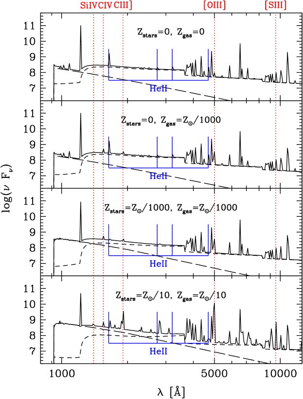
Figure 1: The synthetic spectrum of a zero-metallicity HII region (top panel) is compared to that of HII regions with various combinations of stellar and nebular metallicities (lower panels). The long-dashed and short-dashed lines represent the stellar and nebular continua, respectively.

In Panagia et al. (2004, in preparation) we report on our calculations of the properties of primordial, zero-metallicity HII regions (e.g.,  Figure 1). We find that the electron temperatures is in excess of 20,000 K and that 45% of the total luminosity is converted into the Ly-$\alpha$ line, resulting in a Ly-$\alpha$ equivalent width (EW) of 3000 Å (Bromm, Kudritzki & Loeb 2001). The helium lines are also strong, with the HeII $\lambda$1640 intensity comparable to that of H$\beta$ (Tumlinson et al. 2001, Panagia et al. 2004, in preparation). An interesting feature of these models is that the continuum longwards of Ly-$\alpha$ is dominated by the two-photon nebular continuum. The H$\alpha$/H$\beta$ ratio for these models is 3.2. Both the red continuum and the high H$\alpha$/H$\beta$ ratio could be naively (and incorrectly) interpreted as a consequence of dust extinction even though no dust is present in these systems.

From the observational point of view one will generally be unable to measure a zero-metallicity but will usually be able to place an upper limit to it. When would such an upper limit be indicative that one is dealing with a population III object? According to Miralda-Escudé & Rees (1998) a metallicity Z$\simeq 10^{-3}Z_{\odot}$ can be used as a dividing line between the pre- and post-re-ionization Universe. A similar value is obtained by considering that the first supernova (SN) going off in a primordial cloud will pollute it to a metallicity of $\sim 0.5\times 10^{-3}Z_{\odot}$ (Panagia et al. 2004, in preparation). Thus, any object with a metallicity higher than $\sim 10^{-3}Z_{\odot}$ is not a true first generation object.

3 Low Metallicity HII Regions

We have also computed model HII regions for metallicities from three times solar down to $10^{-6}Z_{\odot}$ (Panagia et al. 2004, in preparation). In Figure 1 the synthetic spectrum of an HII region with metallicity $10^{-3}Z_{\odot}$ (third panel from the top) can be compared to that of an object with zero metallicity (top panel). The two are very similar except for a few weak metal lines. It is also apparent that values of EW in excess of 1,000Å are possible already for objects with metallicity $\sim 10^{-3}Z_{\odot}$. This is particularly interesting given that Ly-$\alpha$ emitters with large EW have been identified at z=5.6 (Rhoads & Malhotra 2001).

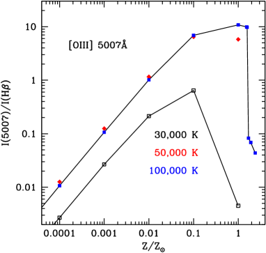
Figure 2: The ratio [OIII]$\lambda 5007$ / H$\beta$ is plotted as a function of metallicity for three different stellar temperatures: 30,000K (open squares and lower line), 50,000K (solid diamonds), and 100,000K (solid squares and upper line).

The metal lines are weak, but some of them can be used as metallicity tracers. In Figure 2 the intensity ratio of the [OIII]$\lambda 5007$ line to H$\beta$ is plotted for a range of stellar temperatures and metallicities. We notice that for $Z<10^{-2}Z_{\odot}$ this line ratio traces metallicity linearly. Our reference value $Z=10^{-3}$ corresponds to a ratio [OIII]/H$\beta$ = 0.1. The weak dependence on stellar temperature makes sure that this ratio remains a good indicator of metallicity also when one considers the integrated signal from a population with a range of stellar masses.

Another difference between zero-metallicity and low-metallicity HII regions lies in the possibility that the latter may contain dust. For a $Z=10^{-3}Z_{\odot}$ HII region dust may absorb up to 30 % of the Ly-$\alpha$ line, resulting in roughly 15 % of the energy being emitted in the far IR (Panagia et al. 2004, in preparation).

4 How to discover and characterize Primordial HII Regions

It is natural to wonder whether primordial HII regions will be observable with the generation of telescopes currently on the drawing boards. In this section we will focus mostly on the capabilities of the James Webb Space Telescope (JWST; e.g. Stiavelli et al.). Here we consider a starburst with $\sim 10^{6}$ M_⊙ in massive stars(which corresponds to a Ly-$\alpha$ luminosity of $\sim 10^{10}$ L_⊙) as our reference model.

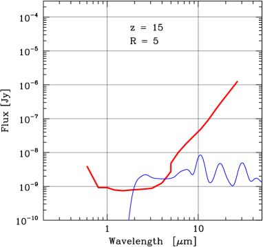
Figure 3: Synthetic spectral energy distribution of a Z=$10^{-3}Z_{\odot}$ starburst object at z=15 containing $10^{6}$ M_⊙ in massive stars (thin line) compared to the imaging limit of $JWST$ at R=5 (thick line). The $JWST$ sensitivity refers to $4\times 10^{5}$ s exposures with S/N=10.

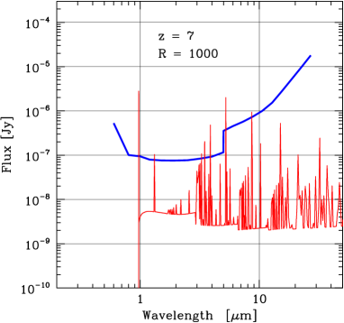
Figure 4: Synthetic spectrum of a Z=$10^{-3}Z_{\odot}$ starburst object at z=7 containing $10^{6}$ M_⊙ in massive stars (thin line) compared to the spectroscopic limit of $JWST$ at R=1000 (thick line). The $JWST$ sensitivity refers to $4\times 10^{5}s$ exposures with S/N=10.

The synthetic spectra, after allowance for IGM HI absorption of the Ly-$\alpha$ radiation (e.g. Miralda-Escudé & Rees 1998, Madau & Rees 2001) and convolution with suitable filter responses are compared to the  JWST imaging sensitivity for $4\times 10^{5}$s exposures in Figure 3. It is clear that JWST will be able to easily detect such objects. Due to the high background from the ground, JWST will remain superior even to 30m ground based telescopes for these applications.

The synthetic spectra can also be compared to the JWST spectroscopic sensitivity for $4\times 10^{5}s$ exposures (see Figure 4). It appears that while the Ly-$\alpha$ line can be detected up to $z\simeq 15-20$, for our reference source only at relatively low redshifts (z$\sim 7$) can JWST detect other diagnostics lines lines such as HeII 1640Å, and Balmer lines. Determining metallicities is then limited to lower redshifts or to brighter sources.

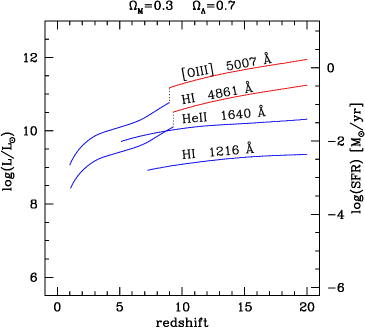
Figure 5: Limiting $total$ luminosity of the ionizing stars (left-hand scale) and top-heavy IMF star formation rate (right-hand scale) to detect various emission lines using $JWST$ spectroscopy, with S/N=10 in integrations of 100 hours, as a function of the source redshift.

We can reverse the argument and ask ourselves what sources can  JWST detect and characterize with spectroscopic observations. Figure 5 displays, as a function of redshift, the total luminosity of a starburst whose lines can be detected with a S/N=10 for a $4\times 10^{5}$s exposure time. The loci for Ly-$\alpha$, HeII 1640Å, H$\beta$, and [OIII] 5007Å are shown. It appears that Ly-$\alpha$ is readily detectable up to z$\simeq$20, the HeII 1640Å line may also be detected up to high redshifts, whereas “metallicity” information, i.e. the intensity ratio I([OIII])/I(H$\beta$), can be obtained at high z only for sources that are $\sim 30$ times more massive or that are magnified $\sim 30$ times by gravitational lensing.

5 Primordial Supernovae

Even if JWST cannot detect individual massive Population III stars, supernova explosions may come to the rescue. In the local Universe supernovae (SNe) can be as bright as an entire galaxy (e.g., Type Ia supernovae (SNIa) at maximum light have M${}_{B}(SNIa)\simeq$-19.5) and are detectable up to large distances. However, SNIa, originating from moderate mass stars, are not expected to occur during the first 1 billion years after Big Bang. In addition, SNIa are efficient emitters only at rest frame wavelengths longer than 2600A, which makes them hard to detect at high redshifts (Panagia 2003a,b). Type II supernovae (SNII) are much more efficient UV emitters but only rarely they are as bright as a SNIa. As a consequence, they will barely be detected at redshifts higher than 10, or, if they are exceptionally bright (à la SN 1979C or SN 1998S) they would be rare events (Panagia 2003a,b).

On the other hand, massive population III stars are much more massive than Pop II or Pop I stars, and the resulting supernovae may have properties very different from those of local Universe SNe. Heger et al (2001) have considered the fate of massive stars in conditions of zero metallicity and have found that for stellar progenitors with masses in the range 140-260 M_⊙ the SN explosions would be caused by a pair-production instability and would be 3 to 100 times more powerful than core-collapse (Type II and Type Ib/c) SNe, so that a Pop III SN at a redshift of z = 20 could attain a peak flux of about 100 nJy at 5 $\mu m$. Such a high flux would be easily detectable with JWST observations made with an integration time of a few hours.

Next point to consider is: “Do Pop III SNe occur frequently enough to be found in a systematic search?” For a standard cosmology ($\Omega_{\Lambda}=0.7$, $\Omega_{m}=0.3$, H${}_{0}=65~{}km~{}s^{-1}Mpc^{-1}$, $\Omega_{b}=0.047$), and assuming that at z=20 a fraction $10^{-6}$ of all baryons goes into stars of 250 M_⊙, Heger et al. (2001) predict an overall rate of 0.16 events per second over the entire sky, or about $3.9\times 10^{-6}$ events per second per square degree. Since for these primordial SNe the first peak of the light curve lasts about a month, about a dozen of these SNe per square degree should be at the peak of their light curves at any time. Therefore, by monitoring about 100 NIRCam fields with integration times of about 10,000 seconds at regular intervals (every few months) for a year should lead to the discovery of three of these primordial supernovae. We conclude that, with a significant investment of observing time (a total of 4,000,000 seconds) and with a little help from Mother Nature (to endorse our theorists views),  JWST will be able to detect individually the very first stars and light sources in the Universe.

References

- [2001] Baraffe I., Heger A., Woosley S. E., 2001, ApJ, 550, 890
- [2001] Bromm V., Ferrara A., Coppi P. S., Larson R. B., 2001, MNRAS, 328, 969
- [2001] Bromm V., Kudritzki R. P., Loeb, A., 2001, ApJ, 552, 464
- [2001] Heger A., Woosley S. E., Baraffe I., Abel T., 2001, astro-ph 0112059
- [2001] Madau P., Rees M. J., 2001, ApJ, 551, L27
- [2001] Marigo P., Girardi L., Chiosi C., Wood P. R. 2001, A&A 371, 252
- [1998] Miralda-Escudé J., Rees M. J., 1998, ApJ, 497, 21
- [2002] Oh S. P., Haiman Z., 2002, ApJ, 569, 558
- [1983] Oliva E., Panagia N., 1983, Ap&SS, 94, 437
- [2003] Panagia N., 2003a, in “Supernovae and Gamma-Ray Bursters”, ed. K. W. Weiler (Berlin: Springer-Verlag), p. 113-144
- [2003] Panagia N., 2003b, STScI Newsletter, Vol. 20, Issue 4, p. 12
- [2001] Rhoads, J. E., Malhotra S., 2001, ApJ, 563, L5
- [2001] Stiavelli, M., et al. 2004, “JWST Primer”, (Baltimore: STScI)
- [2000] Tumlinson J., Shull J. M., 2000, ApJ, 528, L65
- [2001] Tumlinson J., Giroux M. L., Shull J. M., 2001, ApJ, 550, L1