Magnetorotational supernovae

Abstract

We present the results of 2D simulations of the magnetorotational model of a supernova explosion. After the core collapse the core consists of rapidly a rotating proto-neutron star and a differentially rotating envelope. The toroidal part of the magnetic energy generated by the differential rotation grows linearly with time at the initial stage of the evolution of the magnetic field. The linear growth of the toroidal magnetic field is terminated by the development of magnetohydrodynamic instability, leading to drastic acceleration in the growth of magnetic energy. At the moment when the magnetic pressure becomes comparable with the gas pressure at the periphery of the proto-neutron star $\sim 10-15$km from the star centre the MHD compression wave appears and goes through the envelope of the collapsed iron core. It transforms soon to the fast MHD shock and produces a supernova explosion. Our simulations give the energy of the explosion $0.6\cdot 10^{51}$ ergs. The amount of the mass ejected by the explosion is $\sim 0.14M_{\odot}$. The implicit numerical method, based on the Lagrangian triangular grid of variable structure, was used for the simulations.

1 Introduction

The problem of explaining core collapse supernova explosions is one of the long standing and fascinating problems in astrophysics. The most popular core collapse explosion mechanisms up to now were the prompt explosion caused by the bounce shock and the neutrino driven mechanism. The 1D spherically symmetrical simulations of the core collapse supernova do not lead to the explosion (see for example Burrows et al. 1995, Buras et al. 2003 and references therein). The 2D and 3D simulations of the neutrino driven supernova mechanism do not give supernova explosions either with a sufficient level of confidence. The recently improved models of the core collapse where the neutrino transport was simulated by solving the Boltzmann equation do not explode either (Buras et al. 2003).

The important role of the rotation and the magnetic fields for the core collapse supernova was suggested by Bisnovatyi-Kogan (1970). The idea of the magnetorotational mechanism consists of angular momentum transfer outwards using a magnetic field, which twists due to the differential rotation. The toroidal component of the magnetic field amplifies with time, it leads an increase in magnetic pressure and generation of a supernova shock.

The first 2D simulations of the collapse of the rotating magnetized star were presented in the paper of Le Blanck & Wilson (1970), with unrealistically large values of the magnetic field. The differential rotation and amplification of the magnetic field resulted in the formation of the axial jet. A semi-qualitative picture of the magnetorotational explosions was considered by Meier et al. (1976). The results of 2D simulations of the similar problem were given in by Ohnishi (1983) and Symbalisty (1984). Recently, simulations of the magnetorotational processes in the collapsed core have been represented by Kotake et al. (2004) and Yamada & Sawai (2004), where the authors performed 2D simulations of the magnetorotational processes for a strongly magnetized core collapse. They assumed that the initial poloidal magnetic field is uniform and parallel to the rotation axis. In Kotake et al. (2004) the initial strong toroidal magnetic field was also used as the initial condition. In their case the toroidal magnetic field was not equal to zero at the rotational axis $z$, which means a formally nonphysical situation with infinite current density at the rotational axis. The values of the magnetic fields used by them are usual for ”magnetars” but too large for the ordinary core collapse supernova. 1D simulations of the successful magnetorotational supernova explosion for a wide range of the initial values of the magnetic field are represented by Ardeljan et al. (1979). 2D simulations of the magnetorotational explosion in a rotating magnetized cloud have been described by Ardeljan et al. (2000).

One of the main problems for the numerical simulation of the magnetorotational supernova is the smallness of the initial magnetic fields. The ratio of the initial magnetic and gravitational energies is in the range of $10^{-6}-10^{-10}$. This value characterizes the stiffness of the set of MHD equations. We have a problem with strongly varying characteristic timescales. The small one is defined by a very high sound speed in the center of the core and the large one is a characteristic time of the evolution of the magnetic field. In such a situation the explicit numerical methods which are widely used in astrophysical hydro-simulations require an enormously large number of timesteps and a possible loss of accuracy due to the large numerical errors. The implicit approach should be used in this case. It is well known that implicit schemes are free from the Courant timestep limitation, which is too strong for such problems.

At the initial stages of the process the toroidal magnetic field is produced by a twisting of the radial component due to differential rotation and is growing linearly, $B_{\varphi}\sim B_{r}\omega t$. The linear growth is terminated when the toroidal component becomes so strong that magnetohydrodynamic instability starts to develop. This instability leads to poloidal motion of the matter, which increases the radial component, which in turn strongly amplifies the growth of the toroidal field. As a result, both components, toroidal and poloidal, start to grow almost exponentially, shortening greatly the time between the collapse and magnetorotational explosion.

The differential rotation and amplification of the toroidal component of the magnetic field leads to the formation of the MHD compression wave moving from the center of the star. This compression wave goes along a steeply decreasing density profile and soon transforms into the MHD shock wave. This MHD shock is supported by the flux of the matter from the central parts of the star. This matter flux works like a piston increasing the velocity and the strength of the shock. When the MHD shock reaches the outer boundary of the collapsed iron core, the kinetic energy of the radial motion (supernova explosion energy) is $\sim 0.6\cdot 10^{51}$ergs. The amount of mass ejected by the shock is about $0.14M_{\odot}$ of the total mass of the star, $1.2M\odot$.

2 Equations of state and neutrino losses

For the simulations we use the equation of state used in Ardeljan et al. (1987a):

$$P\equiv P(\rho,T)=P_{0}(\rho)+\rho\Re T+\frac{\sigma T^{4}}{3},$$

$$P_{0}(\rho)=\left\{\begin{array}[]{l}P_{0}^{(1)}=b_{1}\rho^{5/3}/(1+c_{1}\rho^{1/3}),0\leq\rho\leq\rho_{1},\\ P_{0}^{(k)}=a\cdot 10^{b_{k}({\textrm{lg}}\rho-8.419)^{c_{k}}},\rho_{k-1}\leq\rho\leq\rho_{k},\\ \hskip 113.81102ptk=\overline{2,6}\\ \end{array}\right.$$ (1)

$$\begin{array}[]{lll}b_{1}=10^{12.40483}&c_{1}=10^{-2.257}&\rho_{1}=10^{9.419}\\ b_{2}=1.&c_{2}=1.1598&\rho_{2}=10^{11.5519}\\ b_{3}=2.5032&c_{3}=0.356293&\rho_{3}=10^{12.26939}\\ b_{4}=0.70401515&c_{4}=2.117802&\rho_{4}=10^{14.302}\\ b_{5}=0.16445926&c_{5}=1.237985&\rho_{5}=10^{15.0388}\\ b_{6}=0.86746415&c_{6}=1.237985&\rho_{6}\gg\rho_{5}\\ a=10^{26.1673},&&\end{array}$$

where $\Re$ is the gas constant equal to $0.83\cdot 10^{8}\frac{\mathrm{cm^{2}}}{\mathrm{s}^{2}}$K, $\sigma$ is the constant of the radiation density, $P$ is pressure, $\rho$ is density, and $T$ is temperature. In the expression $P_{0}(\rho)$ the value $\rho$ was identified with the total mass-energy density. For the cold degenerated matter expression for $P_{0}(\rho)$ is the approximation of the tables from Baym et al. (1971); Malone et al. (1975).

In the neighborhood of points $\rho=\rho_{k}$ in formula (1) the function $P_{0}(\rho)$ was smoothed in the same way as in Ardeljan et al. (1987a), to make continuous the derivative ${\textrm{d}}P_{0}/{\textrm{d}}\rho$ :

$$P_{0}(\rho)=\left\{\begin{array}[]{l}P_{0}^{(k)},\rho\in[\rho_{k-1}+\xi_{k-1},\rho_{k}-\xi_{k}],\\ \hskip 28.45274ptk=\overline{1,6},\>\rho_{0}+\xi_{0}=0,\\ \theta_{k}P_{0}^{(k)}+(1-\theta_{k}P_{0}^{k+1}),\\ \hskip 28.45274pt\rho\in[\rho_{k}-\xi_{k},\rho_{k}+\xi_{k}],k=\overline{1,5},\\ \end{array}\right.$$ (2)

where

$$\theta_{k}=\theta(\rho)=\frac{1}{2}-\frac{1}{2}\sin\left(\frac{\pi}{2\xi_{k}}(\rho-\rho_{k})\right),\quad\xi_{k}=0.01\rho_{k}.$$

The specific energy (per mass unit) was defined thermodynamically as:

$$\varepsilon=\varepsilon_{0}(\rho)+\frac{3}{2}\Re T+\frac{\sigma T^{4}}{\rho}+\varepsilon_{Fe}(\rho,T).$$ (3)

The value $\varepsilon_{0}(\rho)$ is defined by the relation

$$\varepsilon_{0}(\rho)=\int\limits_{0}^{\rho}\frac{P_{0}(\tilde{\rho})}{\tilde{\rho}^{2}}\textrm{d}\tilde{\rho}.$$ (4)

The term $\varepsilon_{Fe}$ in equation (3) is responsible for iron dissociation. It is used in the following form:

$$\varepsilon_{Fe}(\rho,T)=\frac{E_{b,Fe}}{A\>m_{p}}\left(\frac{T-T_{0Fe}}{T_{1Fe}-T_{0Fe}}\right).$$ (5)

It was supposed that in region of the iron dissociation the iron amount was about $50\%$ of the mass, $E_{b,Fe}=8\cdot 10^{-5}$erg is the iron binding energy, $A=56$ is the iron atomic weight, and $m_{p}=1.67\cdot 10^{-24}$g is the proton mass, $T_{0Fe}=0.9\cdot 10^{10}$K, $T_{1Fe}=1.1\cdot 10^{10}$K. For the numerical calculations formula (5) has been slightly modified (smoothed):

$$\varepsilon_{Fe}(\rho,T)=\frac{E_{b,Fe}}{A\>m_{p}}\frac{\left(1+\sin\left(\pi\left(\frac{T-T_{0Fe}}{T_{1Fe}-T_{0Fe}}\right)-\frac{\pi}{2}\right)\right)}{2}.$$ (6)

The neutrino losses for Urca processes are used in the form, taken from Bisnovatyi-Kogan et al. (1976), approximating the table of Ivanova et al. (1969):

$$f(\rho,T)=\frac{1.3\cdot 10^{9}{\textrm{\ae}}(\overline{T})\overline{T}^{6}}{1+(7.1\cdot 10^{-5}\rho\overline{T})^{\frac{2}{5}}}\quad{\textrm{erg}}\cdot{\textrm{g}}^{-1}\cdot{\textrm{s}}^{-1},$$ (7)

$${\textrm{\ae(T)}}=\left\{\begin{array}[]{rclcccccc}1,&\overline{T}<7,\\ 664.31+51.024(\overline{T}-20),&7\leq\overline{T}\leq 20,\\ 664.31,&\overline{T}>20,\end{array}\right.$$ (8)

$$\overline{T}=T\cdot 10^{-9}.$$

The neutrino losses from pair annihilation, photo production, and plasma were also taken into account. These types of the neutrino losses have been approximated by the interpolation formulae from Schindler et al. (1987):

$$Q_{\mathrm{t}ot}=Q_{\mathrm{p}air}+Q_{\mathrm{p}hoto}+Q_{\mathrm{p}lasm}.$$ (9)

The three terms in (9) can be written in the following general form:

$$Q_{d}=K(\rho,\alpha)e^{-c\xi}\frac{a_{0}+a_{1}\xi+a_{2}\xi^{2}}{\xi^{3}+b_{1}\alpha+b_{2}\alpha^{2}+b_{3}\alpha^{3}}.$$ (10)

For $d=pair$, $K(\rho,\alpha)=g(\alpha)e^{-2\alpha}$,

$$g(\alpha)=1-\frac{13.04}{\alpha^{2}}+\frac{133.5}{\alpha^{4}}+\frac{1534}{\alpha^{6}}+\frac{918.6}{\alpha^{8}};$$

For $d=photo$, $K(\rho,\alpha)=(\rho/\mu_{Z})\alpha^{-5};$
For $d=plasm$, $K(\rho,\alpha)=(\rho/\mu_{Z})^{3};$

$$\xi=\left(\frac{\rho/\mu_{Z}}{10^{9}}\right)^{1/3}\alpha.$$

Here, $\mu_{Z}=2$ is the number of nucleons per electron. Coefficients $c,\>a_{i},$ and $b_{i}$ for the different losses are given in the Table 1 from Schindler et al. (1987).

Table 1: Coefficients for formula (10) from Schindler et al. (1987).

	$a_{0}$	$a_{1}$	$a_{2}$	$b_{1}$	$b_{2}$	$b_{3}$	$c$
$10^{8}\>{\textrm{K}}\leq T\leq\>10^{10}\>{\textrm{K}}$
pair	5.026(19)	1.745(20)	1.568(21)	9.383(-1)	-4.141(-1)	5.829(-2)	5.5924
photo	3.897(10)	5.906(10)	4.693(10)	6.290(-3)	7.483(-3)	3.061(-4)	1.5654
plasm	2.146(-7)	7.814(-8)	1.653(-8)	2.581(-2)	1.734(-2)	6.990(-4)	0.56457
$10^{10}\>{\textrm{K}}\leq T\leq\>10^{11}\>{\textrm{K}}$
pair	5.026(19)	1.745(20)	1.568(21)	1.2383	-8.1141(-1)	0.0	4.9924
photo	3.897(10)	5.906(10)	4.693(10)	6.290(-3)	7.483(-3)	3.061(-4)	1.5654
plasm	2.146(-7)	7.814(-8)	1.653(-8)	2.581(-2)	1.734(-2)	6.990(-4)	0.56457

The general formula for the neutrino losses in a nontransparent star has been written in the form, used by Ardeljan et al. (2004):

$$F(\rho,T)=(f(\rho,T)+Q_{tot})e^{-\frac{\tau_{\nu}}{10}}.$$ (11)

The multiplier $e^{-\frac{\tau_{\nu}}{10}}$ in formula (11), where $\tau_{\nu}=S_{\nu}nl_{\nu}$, restricts the neutrino flux for non zero depth to neutrino interaction with matter $\tau_{\nu}$. The cross-section for this interaction $S_{\nu}$ was presented in the form:

$$S_{\nu}=\frac{10^{-44}T^{2}}{(0.5965\cdot 10^{10})^{2}},$$

the concentration of nucleons is

$$n=\frac{\rho}{m_{p}}.$$

The characteristic length scale $l_{\nu}$, which defines the depth for the neutrino absorbtion, was taken to be equal to the characteristic length of the density variation as:

$$l_{\nu}=\frac{\rho}{|\nabla\rho|}=\frac{\rho}{\left((\partial\rho/\partial r)^{2}+(\partial\rho/\partial z)^{2}\right)^{1/2}}.$$ (12)

The value $l_{\nu}$ monotonically decreases when moving to the outward boundary; its maximum is in the center. It approximately determines the depth of the neutrinoabsorbing matter. The multiplier $1/10$ in the expression $e^{-\tau_{\nu}\frac{1}{10}}$ was applied because in the degenerate matter of the hot neutron star only some of the nucleons with the energy near Fermi boundary, approximately $1/10$, take part in the neutrino processes.

3 Basic equations

Consider a set of magnetohydrodynamical equations with selfgravitation and infinite conductivity:

$$\frac{{\rm d}{\bf x}}{{\rm d}t}={\bf v},$$

$$\frac{{\rm d}\rho}{{\rm d}t}+\rho\nabla\cdot{\bf v}=0,$$

$$\rho\frac{{\rm d}{\bf v}}{{\rm d}t}=-{\rm grad}\left(P+\frac{{\bf H}\cdot{\bf H}}{8\pi}\right)+\frac{\nabla\cdot({\bf H}\otimes{\bf H})}{4\pi}-\rho\nabla\Phi,$$

$$\rho\frac{{\rm d}}{{\rm d}t}\left(\frac{{\bf H}}{\rho}\right)={\bf H}\cdot\nabla{\bf v},\>\Delta\Phi=4\pi G\rho,$$ (13)

$$\rho\frac{{\rm d}\varepsilon}{{\rm d}t}+P\nabla\cdot{\bf v}+\rho F(\rho,T)=0,$$

$$P=P(\rho,T),\>\varepsilon=\varepsilon(\rho,T),$$

where $\frac{\rm d}{{\rm d}t}=\frac{\partial}{\partial t}+{\bf v}\cdot\nabla$ is the total time derivative, ${\bf x}=(r,\varphi,z)$, ${\bf v}=(v_{r},v_{\varphi},v_{z})$ is the velocity vector, $\rho$ is the density, $P$ is the pressure, ${\bf H}=(H_{r},\>H_{\varphi},\>H_{z})$ is the magnetic field vector, $\Phi$ is the gravitational potential, $\varepsilon$ is the internal energy, $G$ is gravitational constant, ${\bf H}\otimes{\bf H}$ is the tensor of rank 2, and $F(\rho,T)$ is the rate of neutrino losses.

$r$, $\varphi$, and $z$ are spatial Lagrangian coordinates, i.e. $r=r(r_{0},\varphi_{0},$ and $z_{0},t)$, $\varphi=\varphi(r_{0},\varphi_{0},z_{0},t)$, and $z=z(r_{0},\varphi_{0},z_{0},t)$, where $r_{0},\varphi_{0},z_{0}$ are the initial coordinates of material points of the matter.

Taking into account symmetry assumptions ($\frac{\partial}{\partial\varphi}=0$), the divergency of the tensor ${\bf H}\otimes{\bf H}$ can be presented in the following form:

$${\rm\nabla\cdot}({\bf H}\otimes{\bf H})=\left(\begin{array}[]{l}\frac{1}{r}\frac{\partial(rH_{r}H_{r})}{\partial r}+\frac{\partial(H_{z}H_{r})}{\partial z}-\frac{1}{r}H_{\varphi}H_{\varphi}\\ \frac{1}{r}\frac{\partial(rH_{r}H_{\varphi})}{\partial r}+\frac{\partial(H_{z}H_{\varphi})}{\partial z}+\frac{1}{r}H_{\varphi}H_{r}\\ \frac{1}{r}\frac{\partial(rH_{r}H_{z})}{\partial r}+\frac{\partial(H_{z}H_{z})}{\partial z}\end{array}\right).$$

Axial symmetry ($\frac{\partial}{\partial\varphi}=0$, $r\geq 0$) and symmetry to the equatorial plane ($z\geq 0$) are assumed. The problem is solved in the restricted domain. At $t=0$ the domain is restricted by the rotational axis $r\geq 0$, equatorial plane $z\geq 0$, and outer boundary of the star where the density of the matter is zero, while poloidal components of the magnetic field $H_{r}$, and $H_{z}$ can be non-zero.

We assume axial and equatorial symmetry ($r\geq 0,\>z\geq 0$). At the rotational axis ($r=0$) the following boundary conditions are defined: $(\nabla\Phi)_{r}=0,\>v_{r}=0$. At the equatorial plane ($z=0$) the boundary conditions are: $(\nabla\Phi)_{z}=0,\>v_{z}=0$. At the outer boundary (boundary with vacuum) the following condition is defined: $P_{\textrm{outer boundary}}=0$.

We avoid explicit calculations of the function $\varepsilon_{0}(\rho)$ in (4), because this term is eliminated from (13) due to adiabatic equality:

$$\rho\frac{{\rm d}\varepsilon_{0}}{{\rm d}t}=-\frac{P_{0}}{\rho}\frac{{\rm d}\rho}{{\rm d}t}=P_{0}\nabla\cdot{\bf v},$$ (14)

determining the fully degenerate part of EOS. Therefore, defining

$$\varepsilon^{*}=\frac{3}{2}\Re T+\frac{\sigma T^{4}}{\rho}+\varepsilon_{Fe}(\rho,T),$$

$$P^{*}=\rho\Re T+\frac{\sigma T^{4}}{3}.$$

The equation for the internal energy in (13) can be written in the following form:

$$\rho\frac{{\rm d}\varepsilon^{*}}{{\rm d}t}+P^{*}\nabla\cdot{\bf v}+\rho F(\rho,T)=0.$$ (15)

4 Dimensionless form of equations

For the simulations we rewrite the set of equations (13) in the dimensionless form. The basic scale values are:

$$r_{0}=1.35\cdot 10^{8}\textrm{cm},\>\rho_{0}=10^{9}{\textrm{g/cm}}^{3},$$

$$G=6.67\cdot 10^{-8}{\textrm{cm}^{3}}/({\textrm{g$\cdot$s}^{2}}).$$ (16)

The dimensional functions can be represented in the following way (values with $\tilde{\phantom{a}}$ tilde sign are dimensionless values):

$$r=\tilde{r}r_{0},\>z=\tilde{z}r_{0},\>\rho=\tilde{\rho}\rho_{0},\>v=\tilde{v}v_{0},$$

$$t=\tilde{t}t_{0},\>v_{r}=\tilde{v}_{r}v_{0},\>v_{\varphi}=\tilde{v}_{\varphi}v_{0},\>v_{z}=\tilde{v}_{z}v_{0},\>p=\tilde{p}p_{0},$$ (17)

$$T=\tilde{T}T_{0},\Phi=\tilde{\Phi}\Phi_{0}=\tilde{\Phi}4\pi G\rho_{0}r_{0}^{2},\>\varepsilon=\tilde{\varepsilon}\varepsilon_{0},\>H=\tilde{H}H_{0},$$ (18)

where

$$v_{0}=\sqrt{4\pi G\rho_{0}r_{0}^{2}}=3.908\cdot 10^{9}\textrm{cm/s},$$

$$t_{0}=\frac{r_{0}}{v_{0}},\>p_{0}=\rho_{0}v_{0}^{2},\>T_{0}=\frac{v_{0}^{2}}{\Re},$$

$$\Phi_{0}=4\pi G\rho_{0}r_{0}^{2},\>\varepsilon_{0}=v_{0}^{2},\>H_{0}=\sqrt{p_{0}}=x_{0}t_{0}^{-1}\rho_{0}^{-1}.$$

Taking into account (15) the set of basic equations (13) can be written in the following dimensionless form (the tilde sign $\tilde{\phantom{a}}$ being omitted here):

$$\frac{{\rm d}{\bf x}}{{\rm d}t}={\bf v},$$

$$\frac{{\rm d}\rho}{{\rm d}t}+\rho\nabla\cdot{\bf v}=0,$$

$$\rho\frac{{\rm d}{\bf v}}{{\rm d}t}=-{\rm grad}\left(P+\frac{{\bf H}\cdot{\bf H}}{8\pi}\right)+\frac{\nabla\cdot({\bf H}\otimes{\bf H})}{4\pi}-\rho\nabla\Phi,$$

$$\rho\frac{{\rm d}}{{\rm d}t}\left(\frac{{\bf H}}{\rho}\right)={\bf H}\cdot\nabla{\bf v},\>\Delta\Phi=\rho,$$ (19)

$$\rho\frac{{\rm d}\varepsilon^{*}}{{\rm d}t}+P^{*}\nabla\cdot{\bf v}+\rho F(\rho,T)=0,$$

$$P=P(\rho,T),\>\varepsilon=\varepsilon(\rho,T),$$

5 Initial conditions

We have used the model I from Ardeljan et al. (1987a) as initial conditions . At first we calculated spherically symmetrical stationary model with central density $\rho_{c}=4.5\cdot 10^{9}\textrm{g/cm}^{3}$. The value of the central density corresponds to the maximum in the dependence of the stellar mass on the central density $M_{\textrm{s}}(\rho_{c})$ for $T=0$. The mass of such a spherical star is $M=1,0042M_{\odot}$.

To define the initial model the density (and hence the mass) of the star was increased by 20% at every point. The temperature in the star was defined by the relation: $T=\delta\rho^{2/3}$, where $\delta=1(\textrm{K}\cdot\textrm{cm}^{2}\cdot\textrm{g}^{-2/3})$. At the initial time moment $t=0$, the rigid-body rotation with the angular velocity $\omega=2.519\>\textrm{c}^{-1}$ (rotational period is $\tau=2.496\>\textrm{c}$) was accepted. At $t=0$ we suppose also that $v_{r}=v_{z}=0$. The initial rotational energy is 0.571% of the gravitational energy, and the initial internal energy including the energy of degeneracy is 72.7% of the gravitational energy. The defined initial model is unstable against collapse, and immediately after the beginning of the calculations it starts to contract.

The initial magnetic field (the initial magnetic field which was ”turned on” after the collapse stage) was defined exactly in the same way as in Ardeljan et al. (2000). We define the toroidal current $j_{\varphi}$ in the following form:

$$j_{\varphi}=\left\{\begin{array}[]{l}j_{\varphi}^{u}\>{\rm for}\>z\geq 0,\>r^{2}+z^{2}\leq 0.025^{2},\\ j_{\varphi}^{d}\>{\rm for}\>z\leq 0,\>r^{2}+z^{2}\leq 0.025^{2},\\ 0\>\>\>\>{\rm for}\>{\phantom{z\leq 0,}}\>r^{2}+z^{2}\geq 0.025^{2},\end{array}\right.\\$$ (20)

where

$$j_{\varphi}^{u}=A_{j}\Big{[}{\rm sin}\left(\pi{r\over 0.025}-{\pi\over 2}\right)+1\Big{]}\Big{[}{\rm sin}\left(\pi{z\over 0.025}-{\pi\over 2}\right)+1\Big{]}$$

$${}\times\Big{[}1-\left({r\over 0.025}\right)^{2}-\left({z\over 0.025}\right)^{2}\Big{]},$$

$$j_{\varphi}^{d}=-j_{\varphi}^{u}.{}$$

$A_{j}$ is a coefficient used for adjusting the values of the initial toroidal current and, hence, the magnetic field. After the collapse of the core and obtaining the differentially rotating stationary configuration without a magnetic field. we calculated the initial poloidal magnetic field $H_{r0},H_{z0}$ using the Bio-Savara law. The calculated magnetic field is divergence-free but not force-free and not balanced with other forces. To make it balanced we use the following method (Ardeljan et al. 2000): we ”turn on” the poloidal magnetic field $H_{r0},\>H_{z0}$, but ”switch off” the equation for the evolution of the toroidal component $H_{\varphi}$ in (13). In fact this means that we define $H_{\varphi}\equiv 0,\>{{\rm d}H_{\varphi}\over{\rm d}t}\equiv 0$. From the physical point of view it means that we allow magnetic field lines to slip through the matter of the star in the toroidal direction $\varphi$. After ”turning on” such a field, we let the cloud come to a steady state, where magnetic forces connected with the purely poloidal field are balanced by other forces. The calculated balanced configuration has a magnetic field of quadrupole-like symmetry. The relation of the magnetic energy of the star to its gravitational energy at the moment of the formation of the balanced poloidal magnetic field is $10^{-6}$.

6 Numerical method

The implicit operator-difference completely conservative scheme on the triangular grid of variable structure was used for the numerical modeling of the problem of the magnetorotational supernova explosion. The scheme was suggested and investigated by Ardeljan et al. (1987b) and in earlier papers by these authors.

The solution of the problem is a sequence of time steps. Calculation of every time step can be divided into two parts.

The first part is the calculation of the values of the functions on the next time level using the implicit completely conservative operator-difference scheme on the triangular grid in Lagrangian variables (1995), Ardeljan et al. (1987b). The coordinates of grid knots are changing at this stage.

The second part is an analysis of the quality of the grid, its improvement and adaptation (grid reconstruction). The improvement of the quality of the grid is necessary because of the appearance of ”poor” cells, i.e. triangles which strongly deviate from equilateral triangles. The dynamical adaptation of the grid allows us to concentrate the grid in the regions of the computational domain where spatial resolution needs to be increased and rarefy the grid in the regions where the flow is smooth. It allows us to reduce significantly the dimensionality of the grid and hence strongly reduce the computation time.

The grid reconstruction procedure itself consists of the following stages. The first stage is a local correction of the structure of the grid. The second stage is a calculation of the values of the functions defined in cells in the regions of the corrected structure.

The local correction of the structure of the grid can be done using the following three local operations (see details in Ardeljan et al. (1996)):

1. replacement of the diagonal of the quadrangle formed by two triangles by another diagonal;

2. joining up of two neighboring grid knots;

3. adding of the knot at the middle of the cell side which connects two knots.

The improvement of the grid structure is made using the first two operations. The grid adaptation is made by application of the local operations (II) and (III). The plots which clearly explain these operations are given in Ardeljan et al. (1996).

The values of functions defined in cells and knots involved in grid structure modification are calculated at the second stage of the grid reconstruction.

The application of simple interpolation for the calculations of new values of the grid function leads to the violation of the conservation laws and adds significant errors in the regions with high gradients (for example at shock waves). The goal of the calculation of the new values of functions is to minimize numerical errors introduced by this procedure. To achieve this goal not only the error in the values of the functions but also on their gradients have to be minimized. It is important to fulfill conservation laws (mass, momentum, energy, magnetic flux) in the vicinity of the local grid reconstruction. The method for the calculation of these new values of grid functions is based on a minimization of the functionals containing the values of the functions, its gradients, and grid analogs of the conservation laws (1995).

For the solution we have used the method of the conditional minimization of the functionals guaranteeing exact fulfilment of the conservation laws.

It is important to fulfill conservation laws for the solution of the collapse and magnetorotational supernova explosion problems, because a large number of the time steps need to be made. In such a situation even slight violation of the conservation laws at a time step could lead to a significant growth in the errors and hence to a qualitative distortion of the results.

The method of calculating hydrodynamical values $\rho$ and $P$ during grid reconstruction is taken from (1995). To obtain a better precision some changes have been made in the calculation of the magnetic field components in comparison with our calculations of the collapse of magnetized cloud (Ardeljan et al. (2000)). Earlier, for the calculation of the new values of the magnetic field components we conserved the sum of the products of the magnetic field components values and the volumes of the cells in the vicinity of the reconstructed part of the grid. In this paper we conserve the poloidal magnetic energy and the toroidal magnetic flux in the vicinity of the reconstructed part of the grid.

The grid reconstruction procedure allows us not only to ”correct” the Lagrangian grid, but also to dynamically adapt it using different criteria for the grid in different parts of the computational domain. The grid can be refined in the regions where it is necessary and therefore we can increase the accuracy of the calculations. It is possible to rarefy the grid in those parts of the computational domain where the flow is ”smooth”. The procedure of the rarefying of the grid allows us to significantly reduce the dimension of the grid while preserving the same accuracy for the numerical solution.

Geometrical criteria can be used for the grid adaptation (i.e. restrictions on the length of the cell size, which are defined by the cell coordinates only), but such adaptation criteria are suitable for the flows of simple or easily predictable structures only.

For grid adaptation in the case of complicated flows or flows with unknown structures it is better to apply dynamical criteria which are defined by the solution behavior. The dynamical criteria for the grid adaptation applied here was suggested by Ardeljan et al. (1996).

The characteristic length of the cell side $l_{k}$ was chosen as a local criterion for the grid reconstruction. As an example, consider the criterion where $l_{k}$ is a function of $\rho$ and grad$\rho$. Let’s introduce the function:

$$f(\rho,{\rm grad}\rho)=\frac{\alpha}{(\rho+\varepsilon)^{\gamma_{1}}}+\frac{\beta}{(|{\rm grad}\rho|+\varepsilon)^{\gamma_{2}}},$$ (21)

where $0<\varepsilon<<1,\>\alpha\geq 0,\>\beta\geq 0,\>\alpha+\beta=1$. $\gamma_{1},\>\gamma_{2}$ are power indexes, and ${\rm grad}\rho$ is the grid analog of the density gradient. In limited cases:

$\alpha=1,\>\beta=0,\>f$ depends on the density only;

$\alpha=0,\>\beta=1,\>f$ depends on the gradient of the density only.

Let $N$ be the total number of the grid cells. The characteristic length of the side $l_{k}$ of the cell with the number $k$ will be calculated as a function of the density, the gradient of the density, and the coordinates $r,\>z$ (implicitly) by the following formula

$$l_{k}=2\sqrt{\frac{s_{k}}{3}},\>\>s_{k}=\frac{f(\rho_{k},\>{\rm grad}\rho_{k})}{\sum\limits_{n=1}^{N}f(\rho_{n},\>{\rm grad}\rho_{n})}S.$$ (22)

Here, $S$ is a square of the computational domain, which consists of the triangular cells. The summation in the denominator is made for all grid cells. Note that $S=\sum\limits_{k=1}^{N}s_{k}$, where $s_{k}$ is equal to the square of the equilateral triangle with the length of the side $l_{k}$. In our calculations the function $f$ in formula (21) was used in the following form $f(\rho_{k})=1/(\rho_{k}+\varepsilon)^{0.5}$.

The criterion described was applied in the following way. In the case where the length of the side of the cell $i$ is larger than $2l_{k}$, a new knot is added to the middle of this side of the cell. In the case where the length of the side of the cell $i$ is less than $0.7l_{k}$, the operation of the joining up of these knots is applied. The application of the dynamical adaptation criterion described allowed us not only to adapt the grid to the specialities of the solution but also to provide an acceptable accuracy of the calculations with a small fluctuation of the total number of grid knots and cells. In the calculations described the total number of knots (5000) and cells (10000) was violated not more than 5%.

At the moment of the maximum compression (for the collapse problem) the minimal size of the cell side is so small that application of the uniform grid with the same spatial resolution would require a grid with the dimension $\sim 1000\>\times\>1000$ (!) cells.

The calculation of the gravitational potential in this paper as in Ardeljan et al. (2004) in the frames of the applied numerical method is made on the base of the finite element method of higher order (Zenkevich & Morgan (1983)). This procedure allowed us to increase the accuracy of the calculations and to eliminate the loss of approximation near the $z$ axis.

The linear artificial viscosity (e.g., 1992) was introduced into the numerical scheme for the shock capturing.

7 Results

The simulation of the magnetorotational supernova is divided into two separate parts. The first part is the core collapse simulation, and the second is the ”switching on” of the initial poloidal magnetic field following amplification of its toroidal component $H_{\varphi}$, which is finished by the magnetorotational explosion. The duration of the second phase is defined by the value of the initial magnetic field. The weaker the initial poloidal magnetic field, the longer the stage of the amplification of the toroidal component until the supernova explosion. The results of 1D simulations of the magnetorotational mechanism made by Bisnovatyi-Kogan et al. (1976) and Ardeljan et al. (1979) show that the time from the beginning of the magnetic field evolution to the explosion is proportional to $1/\sqrt{\frac{E_{mag0}}{E_{grav0}}}$, where $E_{mag0}$ and $E_{grav0}$ are initial magnetic and gravitational energies of the star, respectively.

7.1 Core collapse simulation

The core collapse simulation was described in detail in Ardeljan et al. (2004). In the present paper we describe briefly the obtained results. The ratios between the initial rotational and gravitational energies and between the internal and gravitational energies of the star are the following:

$$\frac{E_{rot}}{E_{grav}}=0.0057,\>\frac{E_{int}}{E_{grav}}=0.727.$$

Soon after the beginning of the contraction at $t=0.1377$s at the distance  $6\cdot 10^{5}$cm the bounce shock wave appears. Behind the shock front the temperature of the matter rises sharply and neutrino losses are ”switching on”. In Fig. 1 the time evolution of the neutrino losses is presented.

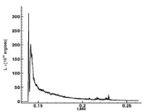
Figure 1: Time evolution of the neutrino luminosity $\int\limits_{0}^{M_{core}}f(\rho,T)dm$ during collapse.

The matter of the star from the outside of the shock wave continues to collapse towards the center of the star.

At $t=0.1424$s the density in the center of the star reaches its maximum value $\rho_{c,max}=5.655\cdot 10^{14}$g/cm³. The matter of the envelope which has passed through the bounce shock wave forms the core (proto-neutron star). Behind the shock front the intensive mixing of the matter takes place.

The shock wave moves through the envelope and at $t=0.2565$s reaches the outer boundary of our computational domain near rotational axis $z$. The shock leads to the ejection of $0.041\%$ of the core mass and $0.0012\%$ ($2.960\cdot 10^{48}$erg) of the gravitational energy of the star. The particles of the matter are treated as ”ejected” when their kinetic energy becomes larger than their gravitational energy and the velocity vector is directed from the star center ($r=0,\>z=0$). The amounts of the ejected mass and energy are too small to explain the core collapse supernova explosion. It should be noted that in Janka & Plewa (2002), where the neutrino losses were calculated using the solution of the Boltzmann equation, the shock wave does not lead to the ejection of the matter. At the final stage of the core collapse ($t=0.261$s.) we obtain a differentially rotating configuration. The central proto-neutron star with a radius $\sim 12.8$km rotates almost rigidly with the rotational period 0.00152s. The angular velocity rapidly decreases with the increase in the distance from the star center. The particles of the matter situated at the outer boundary in the equatorial plain rotate with the period $\sim 35$s (Fig. 2).

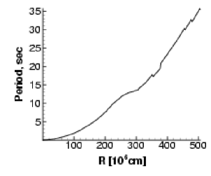
Figure 2: Dependence of the rotational period (in s.) from $r$ coordinate in the equatorial plane ($z=0$) after the collapse for $t=0.261$s.

7.2 Magnetorotational explosion

The results of the collapse simulations show that the amounts of the mass and energy ejected by the bounce shock wave are too small to explain the supernova explosion.

The small ejecting part of the envelope prevents us from continuing the calculations because of significant increase in the square of the computational domain. To overcome this problem the outer part of the envelope was stopped by artificially reducing its velocity (kinetic energy). This artificial method does not influence the central parts of the collapsed core.

After ”stopping” the ejecting part of the envelope we run our code without the magnetic field to be sure that the configuration formed is not changing in time significantly. We reach the stage where the poloidal kinetic energy of the star is less than $0.00001\%$ of the gravitational energy of the star and remains below that value for 1000 time steps. The shape of the envelope of the star does not change significantly during this test.

At that stage we ”switch on” the initial poloidal magnetic field, defined by the current (20). The energy of this magnetic field was taken to be equal to $\sim 10^{-6}$ of the gravitational energy of the star at the moment of including the magnetic field in our simulations. The poloidal magnetic field, defined by the current (20), is divergence-free, but is not force-free, and ”switching on” that field can lead to the artificial violation of the equilibrium of the star. To reach a steady state of differentially rotating configuration with the balanced poloidal magnetic field we exactly follow the procedure from Ardeljan et al. (2000).

The balanced configuration calculated has the magnetic field of quadrupole-like symmetry. After the formation of the balanced poloidal magnetized configuration we ”switch on” the equation for the evolution of the toroidal component $H_{\varphi}$.

We calculate the evolution of the magnetic field after the collapse stage, because at the developed stage the collapse is rather short in time and newly forming proto-neutron star rotates not as differentially as at the end of the collapse. During the collapse the forming proto-neutron star makes only a few revolutions and the magnetic field, which is initially weak, does not have a significant influence on the flow in the star.

At the moment of ”switching on” the toroidal magnetic field we start a counting the time anew.

At the beginning of the simulations the toroidal component of the magnetic field grows linearly with the time at the periphery of the proto-neutron star. The energy of the toroidal magnetic field grows as a quadratic function (Fig. 3). At the developed stage of the $H_{\varphi}$ evolution ($t=0.04s$) the poloidal magnetic energy begins to grow much faster due to developing magnetorotational instability (Akiyama et al. 2003) leading also to a rapid growth of the poloidal components.

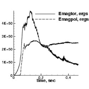
Figure 3: Time evolution of the toroidal and poloidal parts of the magnetic energy during magnetorotational explosion.

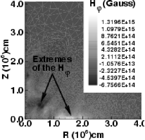
Figure 4: The toroidal field $H_{\varphi}$ distribution after $0.012$s of the beginning of the evolution of the $H_{\varphi}$ in the central part of the star.

Due to the quadrupole-like type of the symmetry of the initial magnetic field the generated toroidal field $H_{\varphi}$ has two extremes. The first is at the equatorial plane and the second is out of the equatorial plane at the periphery of the proto-neutron star closer to the axis of rotation $z$. The two extremes have different signs of $H_{\varphi}$. In Fig. 4 the distribution of the $H_{\varphi}$ is plotted at $0.012$s. These extremes approximately correspond to the extremes of the term $r{\bf H}\cdot{\textrm{g}rad}(V_{\varphi}/r)$ (Ardeljan et al. 2000) in the equation for the evolution of the $H_{\varphi}$, because the star is in a steady state condition, and only this term in this case determines the evolution of $H_{\varphi}$.

The maximal value of the $H_{\varphi}$ reached during the amplification of the toroidal field phase is $\sim 2.5\cdot 10^{16}$G. This maximum is situated at the equatorial plane at a distance $1.7\cdot 10^{6}$ cm from the center of the star, and it is reached at $t=0.058$s. The toroidal part of the magnetic energy decreases with time after reaching its maximal value of $4.8\cdot 10^{50}$ergs at $t=0.12$s. The poloidal magnetic energy at the developed explosion stage is $\approx 2.5\cdot 10^{50}$erg and keeps this value until the end of our simulations (Fig. 4).

The magnetic pressure is highest in the regions where the $H_{\varphi}$ reaches its extremal values. At these regions the $|H\varphi|$ is approximately 100 times higher than the absolute value of the poloidal field ($\sqrt{H^{2}_{r}+H^{2}_{z}}$).

The angular momentum is subtracted by the magnetic torque from the proto-neutron star. The magnetic field works as a ”transmission belt” for the angular momentum. The envelope of the star starts to blow up slowly. The contraction wave appears at the periphery of the proto-neutron star near the extremes of the $H_{\varphi}$. This contraction wave moves along a steeply decreasing density profile. The amplitude of this wave rapidly grows, and after a short time it transforms into the fast MHD shock wave. The growing toroidal magnetic field due to the differential rotation works as a piston for the originated MHD shock. Time evolution of the velocity field $v_{r},\>v_{z}$, specific angular momentum $v_{\varphi}r$, and temperature $T$ for the time moments $t=0.07,0.20,0.30s$ is given in Fig. 5, and Fig. 6.

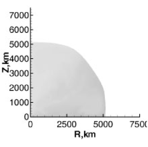
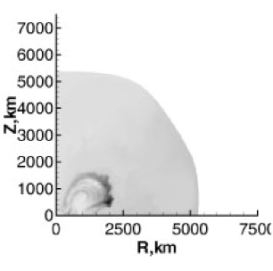
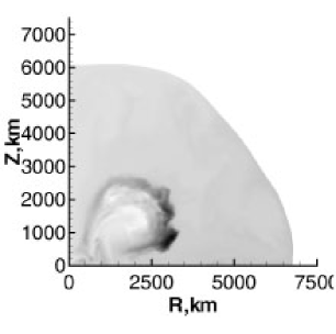
Figure 5: Time evolution of the specific angular momentum $v_{\varphi}r$ for the time moments $t=0.07s,\>0.20s,\>0.30s$. The darker parts of the plots correspond to the higher specific angular momentum.

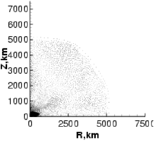
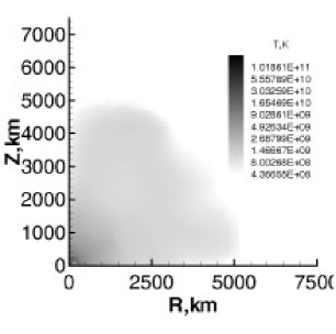
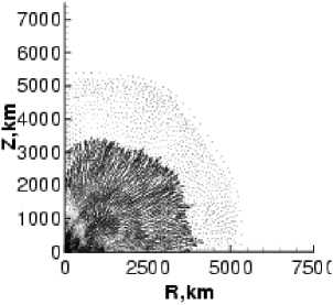
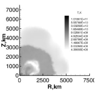
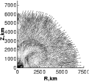
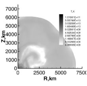
Figure 6: Time evolution of the velocity field (left column) and temperature (right column) for the time moments $t=0.07s,\>0.20s,\>0.30s$.

The flow behind the initial MHD shock is very inhomogeneous. Possible reasons of this inhomogeneity are:

• the aftershock behavior of the gas flow in the presence of the gravitational field,

• the magnetorotational instability appearing at the periphery of the proto-neutron star.

The oscillating structure of the flow behind the shock wave in the gravitational field (without magnetic fields) was investigated analytically in a 1D case in the acoustical approximation by Lamb (1909) and numerically for 1D gravitational gas dynamics by Kosovichev & Popov (1979). Similar oscillating structure was found in our 2D simulations of the collapse of the rapidly rotating cold protostellar cloud (Ardeljan et al. 1996). The main reason for this effect is a change of dispersion properties of the matter in the presence of a gravitational field.

During the evolution of the magnetorotational explosion the proto-neutron star loses angular momentum, contracts and slightly increases its rotation. This leads to the further amplification of the toroidal magnetic field in this region. In other words it means that the ”piston” continues to push the matter from the central object to the envelope and to support the MHD shock. The continuous support of the supernova shock in the magnetorotational mechanism is the main qualitative difference from the prompt shock and neutrino driven supernova mechanisms.

Due to the quadrupole-like type of the symmetry of the initial magnetic field the MHD shock is stronger, and it moves faster near the equatorial plane $z=0$. The matter of the envelope of the star is ejected preferably near the equatorial plane.

The formation of the MHD shock and its propagation leads to the secondary neutrino losses jump (Fig. 7), but now it is much weaker than it was at the collapse stage.

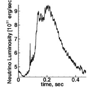
Figure 7: Time dependence of the neutrino luminosity $\int\limits_{0}^{M_{core}}f(\rho,T)dm$ during the magnetorotational explosion.

The integral neutrino losses as a function of time (during magnetorotational stage) is given in the Fig. 8.

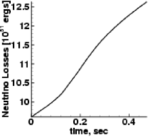
Figure 8: The integral neutrino losses as a function of time during the magnetorotational explosion.

Time dependence of the ejected mass of the star is given in the Fig. 9.

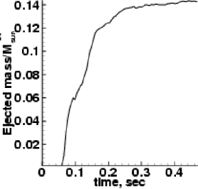
Figure 9: Time dependence of the ejected mass in relation to $M_{\odot}$ during the magnetorotational explosion.

In Fig. 10 the time dependence of the ejected energy is represented. The particle is considered as ejected if its kinetic energy is greater than its potential energy and its velocity vector is directed from the center.

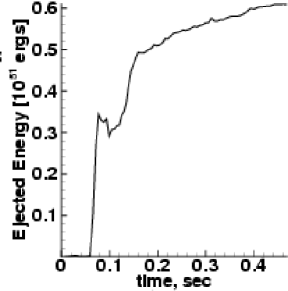
Figure 10: Time dependence of the ejected energy during magnetorotational explosion.

The results of our simulations show that during magnetorotational explosion $\sim 0.14\>M_{\odot}$ of the mass and $\sim 0.6\cdot 10^{51}$ergs are ejected.

The MHD shock which produces the supernova is a fast MHD shock (as in Ardeljan et al. 2000), because its velocity is larger than fast magnetic sound speed in the upstream flow, while the velocity of the slow MHD shock in the downstream flow is between Alfvenic and slow magnetic sound speeds.

The magnetic field transforms part ($\sim 10\%$) of the rotational energy of the star to the radial kinetic energy (explosion energy). The time dependence of the rotational energy and the poloidal part of the kinetic energy are given in Fig. 11.

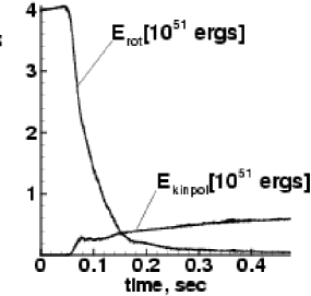
Figure 11: Time dependence of the rotational energy and poloidal kinetic energy of the star during magnetorotational explosion.

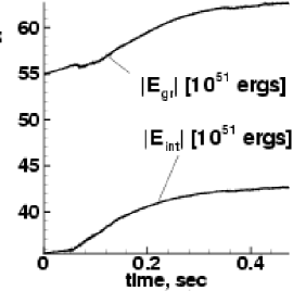
Figure 12: Time dependence of the gravitational and internal energies of the star during magnetorotational explosion.

During the magnetorotational explosion the star loses a significant part of its rotational energy. The rotational energy of the star is transformed not only into the explosion (kinetic energy of radial motion) but is lost in the form of neutrino emission and partially changes the total energy of the star (Fig. 12). The core rotates more slowly now, and it leads to a deeper contraction and some heating of the proto-neutron star.

We stop calculations at $t\approx 9.45s$. At this stage the proto-neutron star rotates with the period $\sim 0.006$s. The absolute value of the poloidal magnetic field at the periphery of the proto-neutron star (at the equatorial plane, $\sim 10$km from the center of the star) is $\sqrt{H_{r}^{2}+H_{z}^{2}}\approx 2\cdot 10^{14}$G.

8 Appearance of the magnetorotational instability in 2-D picture

Magnetorotational instability (MRI) in the magnetized star with differential rotation was analyzed by Spruit (2002), who indicated to dynamo action, accompanies a development of such instability. In our axially symmetric 2D simulations dynamo action is prohibited (Cowling 1957), nevertheless the development of the MRI takes place. It was investigated in 2D numerically for the case of accretion discs by Hawley & Balbus (1991) and Fromang et al. (2004). The possibility of the appearance of such instability was also mentioned by Colgate et al. (1990) in application to the SN1987a. The qualitative picture of the MRI in 2D is the following. At the first stages the differential rotation leads to a linear growth of the toroidal field described qualitatively as

$$\frac{{\mathrm{d}}H_{\varphi}}{{\mathrm{d}}t}=H_{r}\left(r\frac{{\mathrm{d}}\Omega}{{\mathrm{d}}r}\right).$$ (23)

The right side is constant at the initial stage of the process. When toroidal field reaches its critical value $H_{\varphi*}$, the MRI instability starts to develop. As follows from our calculations the critical value corresponds to the relation between toroidal magnetic and internal energy densities as

$$\frac{H^{*2}_{\varphi}}{8\pi}=\frac{1}{10}E\rho.$$ (24)

Appearance of MRI is characterized by formation of multiple poloidal differentially rotating vortexes, which twist the initial poloidal field leading to its amplification according to

$$\frac{{\mathrm{d}}H_{r}}{{\mathrm{d}}t}=H_{r0}\left(\frac{{\mathrm{d}}\omega_{v}}{{\mathrm{d}}l}l\right),$$ (25)

where $l$ is the coordinate, directed along the vortex radius, $\omega_{v}$ is the angular velocity of the poloidal vortex. Qualitatively the poloidal field amplification due to the vortexes induced by MRI is shown in the Fig. 13.

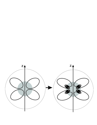
Figure 13: Qualitative picture of the development of the magnetorotational instability.

The enhanced poloidal field immediately starts to take part in the toroidal field amplification according to (23). With further growing of $H_{\varphi}$ the poloidal vortex speed increases. Our calculations give the values of $\omega_{v}=0.0132\>{\mathrm{s}^{-1}}$ at $|H_{\varphi}|=2.46\cdot 10^{15}{\mathrm{G}}$ corresponding to $t=0.041\>{\mathrm{s}}$ and $\omega_{v}=0.052\>{\mathrm{s}^{-1}}$ at $|H_{\varphi}|=4.25\cdot 10^{15}{\mathrm{G}}$ corresponding to $t=0.052\>{\mathrm{s}^{-1}}$ for the same Lagrangian particle. In general we may approximate the value in brackets (25) by linear function on the value $(H_{\varphi}-H^{*}_{\varphi})$ as

$$\left(\frac{{\mathrm{d}}\omega_{v}}{{\mathrm{d}}l}l\right)=\alpha(H_{\varphi}-H^{*}_{\varphi}).$$ (26)

$H_{r}$(or $H_{poloidal}$ in general case) in (23) is not constant anymore after onset of MRI, but described by (25) and (26). Assuming for the simplicity that $\left(r\frac{{\mathrm{d}\Omega}}{{\mathrm{d}}r}\right)=A$ is constant during the first stages of MRI, and taking $H^{*}_{\varphi}$ as constant we come to the following equation:

$$\frac{{\mathrm{d}}^{2}}{{\mathrm{d}}t^{2}}\left(H_{\varphi}-H^{*}_{\varphi}\right)=AH_{p0}\alpha(H_{\varphi}-H^{*}_{\varphi}),$$ (27)

giving the exponential growth of magnetic field components

$$H_{\varphi}=H^{*}_{\varphi}+H_{p0}e^{\sqrt{A\alpha H_{p0}}(t-t^{*})},$$

$$H_{r}=H_{r0}+\frac{H^{3/2}_{p0}\alpha^{1/2}}{\sqrt{A}}\left(e^{\sqrt{A\alpha H_{p0}}(t-t^{*})}-1\right),$$

taking $H_{p0}$ as seed field for development of MRI.

The above toy model shows the way of development of MRI instability in 2D case. In this case there is no direct influence of toroidal field onto a poloidal one, therefore there is no dynamo action. Nevertheless, both components grow exponentially, chaotically for the poloidal field and both chaotically and regularly for the toroidal one. Magnetorotational explosion is produced by both, regular and chaotic magnetic fields. After rapid neutrino cooling and damping of the hydrodynamic motion, the chaotic component remains frozen into the matter due to high electric conductivity, and chaotic magnetic field could be the source of magnetar activity in soft gamma repeaters Thompson & Beloborodov (2004).

9 Discussion

Our calculations have shown that the magnetorotational mechanism produces enough energy ($0.6\cdot 10^{51}$ergs) to explain the core-collapse supernova of types II and Ib. The Ic type is probably more energetic and could be connected with the collapse of much more massive cores of a few tens of solar masses. The value of the energy production in this particular variant may be considered as a basic one, which may be several times larger or smaller, depending on the mass of the collapsing core, magnetic field intensity and configuration, and rotational energy of the presupernova.

The magnetorotational explosion of a supernova star is divided into three stages:

1. linear growth of the toroidal magnetic field due to the twisting of magnetic field lines,

2. exponential growth of the toroidal and poloidal magnetic fields due to the development of magnetohydrodynamic instabilities (Dungey 1958, Tayler 1973, Spruit 2002),

3. formation of the MHD shock wave and magnetorotational explosion.

The resulting newborn neutron star is characterized by relatively slow rotation: 6 ms in comparison to sub-ms values of the critical rotation. The resulting period could grow with increasing efficiency of the explosion.

The toroidal magnetic energy of the young neutron star decreases more rapidly than the poloidal component which tends to the constant value (see Fig. 3). Possibility of the dynamo action in a similar situation, leading to an increase in the large scale poloidal as well as toroidal components, was considered by Spruit (2002). In our calculations the dynamo action is prohibited due to 2D geometry (Cowling 1957).

Different variants of magnetorotational instability in astrophysics were investigated in connection with jet formation (Lovelace 1976, Meier & Nakamura 2003), and generation of turbulence in the accretion disks (Balbus & Hawley 1998). In the last case the instability of the uniform field, threading the differentially rotating disk is considered, which was investigated earlier in plasma physics (Velikhov 1959, Chandrasekhar 1981).

The large values of the remaining magnetic field in our case are related to the chaotic, nonregular components, which have zeroaverage magnetic flux and could disappear by field annihilation even at large conductivity. The existence of a large chaotic component of magnetic field on a neutron star may last long due to very high conductivity. It may be related the magnetars model or soft gamma repeaters, in which the radiated energy comes from the magnetic field annihilation. Inside the neutron star the regular toroidal, dipole, or quadrupole poloidal components of the magnetic field could remain for a long time, much longer than their chaotic values.

References

- Akiyama et al. (2003) Akiyama S., Wheeler J.C., Meier D.L., Lichtenstadt I., 2003, ApJ, 584, 954
- Ardeljan et al. (1996) Ardeljan N.V., Bisnovatyi-Kogan G.S., Kosmachevskii K.V., Moiseenko S.G., 1996, A&AS, 115, 573
- Ardeljan et al. (2004) Ardeljan N.V., Bisnovatyi-Kogan G.S., Kosmachevskii K.V., Moiseenko S.G., 2004, Astrophysics, 47, 1
- Ardeljan et al. (2000) Ardeljan N.V., Bisnovatyi-Kogan G.S., Moiseenko S.G., 2000, A&A, 355, 1181
- Ardeljan et al. (1979) Ardeljan N.V., Bisnovatyi-Kogan G.S., Popov Yu.P., 1979, Astron. Zh. 56, 1244
- Ardeljan et al. (1987a) Ardeljan N.V., Bisnovatyi-Kogan G.S., Popov Yu.P., Chernigovsky S.V., 1987a, Astron. Zh. 64, 761 (Soviet Astronomy, 1987, 31, 398)
- (7) Ardeljan N.V, Kosmachevskii K.V. 1995, Computational mathematics and modeling, 6, 209
- Ardeljan et al. (1987b) Ardeljan N.V, Kosmachevskii K.V., Chernigovskii S.V., 1987b, Problems of construction and research of conservative difference schemes for magneto-gas-dynamics, MSU, Moscow (in Russian)
- Balbus & Hawley (1998) Balbus S.A., Hawley J.F., 1998, Rev. Mod. Phys., 70, 1
- Baym et al. (1971) Baym G., Pethick C., Sutherland P., 1971, ApJ, 170, 299
- Bisnovatyi-Kogan (1970) Bisnovatyi-Kogan G.S., 1970, Astron. Zh. 47, 813 (Soviet Astronomy, 1971, 14, 652)
- Bisnovatyi-Kogan et al. (1976) Bisnovatyi-Kogan G.S., Popov Yu.P., Samokhin A.A., 1976, ApSS, 41, 321
- Buras et al. (2003) Buras R., Rampp M., Janka H.Th., Kifonidis K., 2003, Phys.Rev.Lett., 90, 241101
- Burrows et al. (1995) Burrows A., Hayes J., Fryxell B.A., 1995, ApJ, 450, 830
- Chandrasekhar (1981) Chandrasekhar S., Hydrodynamic and Hydromagnetic stability New York, Dover,1981
- Colgate et al. (1990) Colgate S.A., Krauss L.M., Shramm D.N., Walker T.P., 1990, Astro. Lett. and Coomunications, 27, 411
- Cowling (1957) Cowling T.G., Magnetohydrodynamics New York, Interscience,1957
- Dungey (1958) Dungey J.W.,1958, Cosmic electrodynamics. Cambridge Univ. Press, Cambridge
- Fromang et al. (2004) Fromang S., Balbus S.A., De Villiers J.P., 2004, ApJ, 616, 357
- Hawley & Balbus (1991) Hawley J.F., Balbus S.A., 1991, ApJ, 376, 223
- Ivanova et al. (1969) Ivanova L.N., Imshennik V.S., Nadezhin D.K., 1969, Nauchn. Inform. Astron. Sov. Akad. Nauk SSSR (Sci. Inf. of the Astr. Council of the Acad. Sci. USSR), 13, 3
- Janka & Plewa (2002) Janka H.-Th., Plewa T., astro-ph/0212314
- Kosovichev & Popov (1979) Kosovichev A.G., Popov Yu.P., 1979, J. Mathem. Phys. Comput. Math. 19,1251
- Kotake et al. (2004) Kotake K., Sawai H., Yamada S., Sato K., 2004, ApJ, 608, 391
- Lamb (1909) Lamb H., 1909, Proc. London math. Soc., 7, 122
- Le Blanck & Wilson (1970) Leblanck L.M., Wilson J.R., 1970, ApJ, 161, 541
- Lovelace (1976) Lovelace R.V.E, 1976, Nature, 262, 649
- Malone et al. (1975) Malone R.C., Johnson M.B., Bethe H.A., 1975, ApJ, 199, 741
- Meier et al. (1976) Meier D.L., Epstein R.I., Arnett W.D., & Schramm D.N. 1976, ApJ, 204, 869
- Meier & Nakamura (2003) Meier D.L., Nakamura M. 2003 in Proc. ”3-D Signatures in Stellar Explosions”, ed. C.Wheeler, astro-ph/0312050
- Ohnishi (1983) Ohnishu N., 1983, Tech. Rep. Inst. At. En. Kyoto Univ., No.198
- (32) Samarskii A.A., Popov Ju.P., 1992, Difference Methods for the Solution of Problems of Gas Dynamics. Moscow, Nauka, (in Russian)
- Schindler et al. (1987) Schinder P.J., Schramm D.N., Wiita P.J., Margolis S.H., Tubbs D.L., 1987, ApJ, 313, 531
- Spruit (2002) Spruit H.C., 2002, A&A, 381, 923
- Symbalisty (1984) Symbalisty E.M.D., 1984, ApJ, 285, 729
- Tayler (1973) Tayler R.J., 1973, MNRAS, 161, 365
- Thompson & Beloborodov (2004) Thompson C., beloborodov A.M., 2005, astro-ph/0408538
- Velikhov (1959) Velikhov E.P., 1959, J. Exper. Theor. Phys., 36, 1398
- Yamada & Sawai (2004) Yamada S., Sawai H., 2004, ApJ, 608, 907
- Zenkevich & Morgan (1983) Zenkevich O.C., Morgan K. Finite elements and approximation. NY, 1983, 318 .