An hydrodynamic shear instability in stratified disks

We discuss the possibility that astrophysical accretion disks are dynamically unstable to non-axisymmetric disturbances with characteristic scales much smaller than the vertical scale height. The instability is studied using three methods: one based on the energy integral, which allows the determination of a sufficient condition of stability, one using a WKB approach, which allows the determination of the necessary and sufficient condition for instability and a last one by numerical solution. This linear instability occurs in any inviscid stably stratified differential rotating fluid for rigid, stress-free or periodic boundary conditions, provided the angular velocity $\Omega$ decreases outwards with radius $r$. At not too small stratification, its growth rate is a fraction of $\Omega$. The influence of viscous dissipation and thermal diffusivity on the instability is studied numerically, with emphasis on the case when $d\ln\Omega/d\ln r=-3/2$ (Keplerian case). Strong stratification and large diffusivity are found to have a stabilizing effect. The corresponding critical stratification and Reynolds number for the onset of the instability in a typical disk are derived. We propose that the spontaneous generation of these linear modes is the source of turbulence in disks, especially in weakly ionized disks.

1 Introduction

The simplest model of an accretion disk is that of a barotropic, axisymmetric rotating shear flow in hydrostatic vertical equilibrium, with a Keplerian velocity law. Realistic disks are also subject to baroclinic effects (when the rotation departs from cylindrical, i.e. when $\Omega$ varies also with the axial coordinate $z$) and to a vertical stratification, induced either by the hydrostatic state or via the illumination of the surface of the disk due to the central object. If the stratification is unstable, it leads to turbulence via convective instability. When the stratification is stable, it is generally ignored or thought to be unimportant in the stability analysis, under the rationale that it can only stabilize the flow. Ignoring the stratification and baroclinic effects makes the accretion disk look like a simple differentially rotating shear flow, with an azimuthal keplerian angular velocity profile $\Omega(r)\propto r^{-3/2}$ . Its linear stability with respect to axisymmetric disturbances is governed by the Rayleigh criterion in the inviscid limit:

$$\frac{d(r^{2}\Omega)^{2}}{dr}>0\quad\hbox{for stability.}$$ (1)

Flows obeying this criterion are called centrifugally stable. Keplerian flow, in which angular momentum increases outwards, falls into this category. Yet, there is observational evidence that astrophysical (putatively Keplerian) disks are turbulent (cf. Hersant et al. 2003), and thus that a source of instability exists in these flows.

Leaving aside baroclinic effects, various mechanisms have been found able to destabilize centrifugally stable flows. They may or may not apply to astrophysical disks.

i) Centrifugally stable flows can experience a globally subcritical bifurcation (Dauchot & Manneville 1997), induced by finite amplitude disturbances involving non-linear mechanisms not captured by the Rayleigh criterion (Dubrulle 1993). The transition threshold in this case is related to the amplitude of the external disturbance, as typically observed in a plane shear flow  (Dauchot & Daviaud 1994 ).

Taylor-Couette experiments, with fluid sheared between two concentric rotating cylinders in the centrifugally stable regime, have revealed such transition. When the inner cylinder is at rest, the data of Wendt (1933) and Taylor (1936), re-analyzed by Richard and Zahn (1999), show that for the typical amplitude of the intrinsic disturbances of the experimental devices, turbulence subcritically sets in as soon as $R=Ud/\nu>R^{nl}_{c}$, where $U$ is the relative velocity between the walls, $d$, the radial extent of the flow (the gap) and $\nu$ the viscosity.

For small curvature, the threshold is essentially independent of the gap/radius ratio and in the limit of plane Couette flow, $R^{nl}_{c}\simeq 1500$, a value in agreement with the minimal Reynolds number for which turbulence can be induced in plane Couette flow. For large curvature, $R^{nl}_{c}$ scales with the square of the gap/radius ratio.

Finally, novel laboratory experiments were performed recently (Richard 2001), to refine the present analysis and to explore regimes with co-rotating cylinders. For the first time, the hysteretic behavior of the transition with the inner cylinder at rest has been described, a signature of subcriticality and turbulent regimes were detected when the angular velocity decreases outward, in the centrifugally stable region.

ii) Centrifugally stable flows can also be destabilized by compressibility effects via non-axisymmetric instabilities (Papaloizou & Pringle 1984). This instability occurs independently of boundary conditions as long as $d\ln\Omega/d\ln r<-\sqrt{3}$ (Papaloizou & Pringle, 1985; Glatzel, 1987). However, the existence of such an instability for Keplerian disks requires the presence of at least one sharp edge (Goldreich & Narayan, 1985). This condition may be unrealistic in standard accretion disks.

iii) Centrifugally stable flows can be further destabilized by adding another restoring force, which acts as a catalyzer. A first example is a vertical magnetic field (Velikhov 1959; Chandrasekhar 1960), which renders such flows unstable provided they are anticyclonic, i.e. if $d(\Omega)^{2}/dr<0$. The application of this mechanism to disks was first discussed by Balbus and Hawley (1991); they showed that the stratification of the disk does not modify the result, and that the maximal growth rate of instability in that case is of the order of the angular rotation velocity in the inviscid limit. The instability of a rotating flow subject to vertical magnetic field includes a surprising paradox: experimentally, it was found that in liquid metals, in the centrifugally unstable case, the magnetic field inhibits instabilities, and thus, has a stabilizing influence (Chandrasekhar 1960). In the centrifugally stable case, it creates an instability. Summarizing, it appears that a stabilizing factor acts upon a stable flow so as to generate instability.

iv) A similar behavior was observed in rotating flows subject to a vertical stable stratification (Whithjack & Chen 1974, Boubnov and Hopfinger, 1995). In the centrifugally unstable case, the stratification enhances the stability of the flow and tends to increase the critical Reynolds number of the inner cylinder (Fig. 1). In the centrifugally stable regime, the experimental stability curve crosses the critical line for the Rayleigh criterion, and turbulence sets in via a non-axisymmetric mechanism. This instability is present in the small gap and wide gap regime, showing that curvature effect do not play a role in the instability mechanism. A possible theoretical explanation for this instability has been given recently by Molemaker et al. (2001) and Yavneh et al (2001). They performed an analytical and numerical stability analysis of a rotating flow in the presence of a stable vertical temperature gradient, and discovered the existence of a linear non-axisymmetric instability for all anticyclonically sheared flows. In their work, they interpret this instability as being caused by the interaction of two edge modes through a mechanism of arrest and phase locking along the boundaries by the mean shear flow.

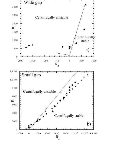
Figure 1: Neutral-stability curves in a stratified Taylor-Couette flow experiment for different stratifications, in the domain $(R_{2},R_{1})$ where $R_{2}$ and $R_{1}$ are the Reynolds numbers based on the gap size and the velocity at the outer or inner cylinder. a) In the wide gap limit (ratio of inner cylinder to outer cylinder equal to $0.2$), experiment of Whithjack and Chen (1974): $N=1.5s^{-1}$ (circles), $N=1.25s^{-1}$ (diamonds) and $N=0.88s^{-1}$ (triangles); b) in the small gap limit (ratio of inner cylinder to outer cylinder equal to $0.8$), experiment of Boubnov and Hopfinger (1995) $N=1.21s^{-1}$ (circles), $N=0.89s^{-1}$ (diamonds), $N=0.54s^{-1}$ (triangles) and $N=0s^{-1}$ (crosses). The continuous line is the neutral-stability line for centrifugal instability computed by Snyder (1968) in an un-stratified Taylor-Couette experiment. In the centrifugally unstable case, one sees that the stratification enhances stability. In the centrifugally stable case, stratification favors instability.

We note that in astrophysical context, the stability of plane rotating shear flow has often been tackled through the so-called shearing sheet transformation introduced by Goldreich and Lynden-Bell (1965). In this approximation, the disk structure is equivalent to a rotating plane Couette flow, with shear being $-3/2$ of the rotation. The advantage of this kind of analysis is the possibility to investigate stability, by using a special class of disturbances for which the stability analysis of this flow can be reduced to study of ordinary differential equations. These modes, first introduced by Lord Kelvin in 1887, have the shape $u(x,y,z,t,k,\beta,k_{z})=u(t)\exp(i(k-S\beta t)x+i\beta y+ik_{z}z)$. Here $S$ is the Couette shear rate, with the flow velocity in the $y$-direction varying with $x$. Individual non-axisymmetric such modes have been found to exhibit algebraic transient growth under various conditions, such as compressibility (Dubrulle & Knobloch 1992) or vertical stable and unstable stratification (Knobloch 1984; Korycansky 1992). However, any amount of dissipation causes ultimate decay of these modes, due to shear winding of the azimuthal wave-numbers. From a theoretical point of view, it can be shown that these modes are associated with the non-normality of the operator governing the perturbation dynamics. They may be the basis of a noise amplification mechanism, resulting in significant angular momentum flux (Ioannou & Kakouris 2001). However, these modes do not form a complete basis (for example, they cannot describe perturbations with periodic boundary conditions in $x$), and their study alone is not sufficient to determine the stability properties of the flow, as recognized by Korycansky (1992). A complete stability analysis requires solving the “initial condition” problem, looking at the stability properties of an infinite superposition of sheared modes, moving with the flow. However, even in the case of non-stratified rotating shear flow, this problem is difficult to handle analytically and calls for a numerical solution (Cambon et al. 1994). Therefore, the shearing-sheet/sheared mode method provides only a partial answer to the stability problem.

In the present paper, we resort to other approaches, in which boundary conditions must be fixed a priori, but which allow for a complete treatment of the instability. Our approach is complementary to the usual sheared mode approximation. We use two classical, analytically tractable approaches to reexamine the instability of a stratified astrophysical disk: one based on the energy method, the second based on the WKB approximation. The energy method is valid for a wide class of boundary conditions, namely rigid (vanishing velocity at the domain boundary), stress free (vanishing velocity derivative at the domain boundary) or periodic boundary conditions in the shear direction. Therefore, it does not apply to individual sheared modes, which satisfy none of these requirements. This method leads to a sufficient condition for stability valid in the inviscid limit, and for perturbations with a characteristic scale much smaller than the vertical scale height (Section 2.1). The influence of curvature on this instability is discussed in Section 2.2. In Section 3, we use a method based on the WKB approximation to derive an explicit solution of the stability problem and exhibit unstable modes in the parameter space covering the sufficient condition for stability. This shows that the sufficient condition for stability is probably necessary. This theoretical study is completed in section 4 by a numerical study, probing instability regimes and the influence of dissipative processes on the instability. This study enlarges the numerical study of Yavneh et al. (2001) towards conditions more typical of astrophysical disks, namely Keplerian velocity profile and finite Prandtl number. In Section 5, we discuss the importance of this mechanism for turbulence generation in disks, and the similarity between this instability and the instability generated by a vertical magnetic field. Our conclusions follow in Section 6, where the interplay between the present shear instability and its baroclinic counterpart is discussed.

2 Theoretical study

We consider a differentially rotating compressible stratified disk. In the following, we focus on perturbations with typical radial scales small compared with the vertical scale height of the disk. This limit provides two simplifications: first, it allows us to consider only the barotropic case, in which all vertical dependence of the equilibrium quantities is ignored. Then it allows elimination of acoustic waves and we can work in the Boussinesq approximation (Korycansky 1992). The dynamical equations ruling the perturbation ${\bf u}$ take then the simple form

$$\nabla\cdot{\bf u} = 0,$$

$$D_{t}{\bf u}+{\bf u}\cdot\nabla{\bf U}+2\Omega{\bf e}_{z}\times{\bf u}+\nabla p-h{\bf g} = \nu\Delta{\bf u},$$

$$D_{t}h+{\bf u}\cdot\nabla H = \frac{\nu}{Pr}\Delta h,$$ (2)

in a frame rotating with the constant angular velocity $\Omega$ (to be chosen later). Here $D_{t}=\partial_{t}+{\bf U}\cdot\nabla$ is the total derivative, $\nu$ is the viscosity, $Pr$ is the Prandtl number, ${\bf g}=\nabla P/\rho$ the local effective gravity, $H$ the basic stratification, and $h$ is the stratification perturbation in the Boussinesq approximation.

The instability we are interested in is present both in rotating Couette flow (Kushner et al. 1998), i.e. for plane geometry, or in Taylor-Couette flow (Molemaker et al. 2001, Yavneh et al. 2001) i.e. for circular geometry. This suggests that curvature effects do not play a role in the instability. To clarify the presentation, we first deal with the simpler, plane case in Section 2.1. In the astrophysical context, this case is equivalent to the so-called shearing sheet approximation of Goldreich and Lynden-Bell (1972). It is also the small gap limit of the Taylor-Couette flow, and is relevant to many laboratory experiments. After discussion of this simple, illustrative case, we come back to the large gap limit (relevant to disks) in Section 2.2, where curvature effects are included. For simplicity, we also consider in this Section only the inviscid limit $\nu=0$, keeping the general case of finite viscosity for numerical exploration (Section 3).

2.1 The plane Couette case

In this case, we assume Cartesian geometry $x,y,z$. The basic flow is a combination of a pure shear flow

$${\bf U}=Sxe_{y},$$ (3)

with a constant rotation $\Omega$ along the $z$ axis.

We expand the perturbation into normal modes: $({\bf u},h)=({\bf\hat{u}},\hat{h})(x)\,\exp[i(\beta y+k_{z}z-\omega t)]$. Plugging this into (2) and noting the velocity perturbation $\hat{\bf u}=(u,v,w)$ and the rescaled entropy perturbation $\gamma\hat{h}=\theta\partial_{z}H$, we obtain the following system:

$$-i\sigma u-2\Omega v = -Dp$$

$$-i\sigma v+Zu = -i\beta p$$

$$-i\sigma w+N^{2}\theta = -ik_{z}p,$$

$$-i\sigma\theta = w,$$

$$Du+i\beta v+ik_{z}w = 0.$$ (4)

Here, we have introduced the $x$-derivative $D$ and the Doppler-shifted frequency $\sigma=\omega-\beta Sx$. The equation also involves the frequency $Z=2\Omega+S$ and the squared Brunt-Väisälä frequency in the axial direction:

$$N^{2}=-{1\over\gamma}g_{z}\,\partial_{z}H,$$ (5)

which is positive in the case of stable stratification. The system of equations (4) also describes a Keplerian disk in the shearing sheet approximation, provided $\Omega$ is the local Keplerian rotation and $Z=\Omega/2$.

The system (4) is a coupled differential system. To investigate the basic mechanism of instability, we use (4) to eliminate three components in order to get a single differential system for one component, say $u$. For this, we first eliminate the pressure by using the three last equations of (4) to get:

$$p=-i\frac{N^{2}-\sigma^{2}}{k_{z}^{2}\sigma}\left(Du+i\beta v\right).$$ (6)

We then substitute this expression into the second equation of (4) to obtain $v$ as a function of $u$. This expression can be used in the first equation of (4) to obtain a closed equation for $u$. After simplification and rearrangements, we obtain finally:

$$D\left(\frac{K}{G}Du\right)+\frac{\beta Z}{\sigma}uD\left(\frac{K}{G}\right)+2k_{z}^{2}\frac{\Omega Z}{G}u-u=0,$$ (7)

where $K=\sigma^{2}-N^{2}$ and $G=(k_{z}^{2}+\beta^{2})\sigma^{2}-\beta^{2}N^{2}$. It is easy to check that this equation is the zero-curvature limit of that derived by Yavneh et al. (2001). Note that both $K$ and $G$ depend on $x$ through $\sigma$.

Eq. (7) is a classical generalized eigen-value problem (corresponding to a linear differential operator) which can be solved once the boundary conditions have been specified. The instability occurs for values of the eigen-values such that $\omega$, and therefore $\sigma$ has a positive imaginary part.

To derive stability conditions, we use an integral method adapted from Chandrasekhar (1960). We first reset equation (7) into a standard shape by the change of function $u=\hat{u}\left(\frac{K}{G}\right)^{-1/2}$ to obtain:

$$D^{2} \hat{u}-E\hat{u}=0,$$ (8)

$$E =\frac{a^{2}}{4}+\frac{Da}{2}-\frac{a\beta Z}{\sigma}-2k_{z}^{2}\frac{\Omega Z}{K}+\frac{G}{K}$$

where $a=D(\ln(K/G)$. We then multiply (8) by the complex conjugate $\hat{u}^{*}$ and integrate over the whole domain. We obtain an integral equation, valid for both rigid ($\hat{u}=0$ at boundaries), free-slip ($Du=0$ at boundaries) or periodic boundary conditions:

$$\int dx\left|D\hat{u}\right|^{2}+\int dx\,E\left|\hat{u}\right|^{2}=0.$$ (9)

Both $\left|D\hat{u}\right|^{2}$, and $\left|\hat{u}\right|^{2}$ are positive continuous real function over the integration domain. The function $E$ is a complex function of $x$ (through $\sigma$) whose real and imaginary part $E_{r}$ and $E_{i}$ are continuous over the integration domain. By continuity (intermediate value theorem), there exist two points $x_{1}$ and $x_{2}$ such that:

$$\int dx\left|D\hat{u}\right|^{2}+E_{r}(x_{1})\int dx\left|\hat{u}\right|^{2}\equiv I_{1}+E_{r}(x_{1})\,I_{0}=0,$$

$$E_{i}(x_{2})\int dx\left|\hat{u}\right|^{2}=0.$$ (10)

In principle, a stability condition may then be found by imposing that there exist no solutions with positive $\omega_{i}$ for any value of $x_{2}$ and $x_{1}$. In practise, the algebraic equation is of order eight in $\omega_{i}$, and we were not able to derive simple explicit stability conditions. We therefore restrict ourselves to the instability condition in the limit of weak non-axisymmetry, by using the fact that $\omega_{i}$ vanishes in the limit $\beta=0$ and that the instability is non-oscillatory $\omega_{r}=0$ (see Molemaker et al, 2001). Then, since $\sigma=-\beta Sx+i\omega_{i}$, we can set $\sigma=\beta\tilde{\sigma}$ and expand $E$ as a function of $\beta$. To first order in $\beta$, we find:

$$\frac{E}{k_{z}^{2}}=2\frac{\Omega Z}{N^{2}}-4\frac{S\Omega}{k_{z}^{2}\tilde{\sigma}^{2}-N^{2}}+3\left(\frac{SN}{k_{z}^{2}\tilde{\sigma}^{2}-N^{2}}\right)^{2}.$$ (11)

To obtain an analytical condition, we set $\rho e^{i\psi}=k_{z}^{2}\tilde{\sigma}^{2}-N^{2}$ and note that finding positive $\omega_{i}$ as a function of $x_{2}-x_{1}$ is equivalent to finding $\rho$ as a function of $\psi$. In these variables, the first equation (10) becomes to first order in $\beta$:

$$\left(\frac{I_{1}}{k_{z}^{2}I_{0}}\frac{N^{2}}{4\Omega^{2}}+\frac{S}{2\Omega}\right)\rho^{2}+\left(\rho-\frac{SN^{2}}{2\Omega}\cos\psi\right)^{2}+\left(\frac{S}{2\Omega}\right)^{2}(5\cos^{2}\psi-3)N^{4}=0.$$ (12)

In the limit of vanishing stratification, the last term of the l.h.s. of eq. (12) is negligible. The second term of the l.h.s. is always positive. So a (sufficient) condition which guarantees the absence of unstable solutions is that the first term of the l.h.s. is positive, i.e.:

$$\frac{S}{2\Omega}>-\frac{1}{4}\frac{I_{1}}{k_{z}^{2}I_{0}}\frac{N^{2}}{\Omega^{2}}\quad\rm{STABILITY}.$$ (13)

Using the energy method, we have derived a sufficient criterion for stability for periodic, stress-free or rigid boundary conditions. Therefore, it does not prove that flows with $S/2\Omega<0$ are unstable. However, in the WKB approximation of Section 3 and numerical stability analysis performed in Section 4, we found that all flows with $S/2\Omega<0$ are unstable. This shows that condition (13) is also a necessary condition for stability for these boundary conditions.

In the limit of vanishing stratification, we find $S/2\Omega>0$ as a criterion for stability, instead of the $S/2\Omega>-1$ criterion for centrifugal stability. The stratification thus enlarges the domain of instability. However, this criterion is non-axisymmetric; for $\beta=0$, the only non-trivial modes are stable, with the epicyclic frequency $\sigma^{2}=(2\Omega Z)k_{z}^{2}$. Note that our criterion is in agreement with the criterion derived by Molemaker et al (2001) and Yavneh et al (2002), which was $S/2\Omega<0$ for instability. Note also that as the stratification increases, it becomes increasingly easy to satisfy (13). So, while a weak stratification destabilizes the flow, a large stratification re-stabilizes it. We show in Section 2.6 that when the stratification is replaced by a vertical magnetic field, a similar phenomenon occurs: weak fields are destabilizing, while very large fields are stabilizing.

2.2 Influence of curvature

We now explore how curvature effects modify the instability. For this, we assume cylindrical coordinates $r,\phi,z$ and consider the stability of a general rotating shear flow

$${\bf U}=r\Omega(r)e_{\phi},$$ (14)

Thus, the rotation frequency is noted $\Omega$, and the shear rate $S=r\partial_{r}\Omega$. The normal-mode decomposition is

$$({\bf u},h)=({\bf\hat{u}},\hat{h})(x)e^{i(l\phi+k_{z}z-\omega t)}.$$ (15)

The analog of (7) in this general case is derived in Yavneh et al 2001. It is:

$$D\left(\frac{K}{G}rD\left(ru\right)\right)$$

$$+\left(\frac{l}{\sigma}D\left(\frac{KZ}{G}\right)+2rk_{z}^{2}\frac{\Omega Z}{G}-\frac{1}{r}\right)(ru)=0,$$ (16)

where $Z=2\Omega+S$, $K=\sigma^{2}-N^{2}$, $G=(r^{2}k_{z}^{2}+l^{2})\sigma^{2}-l^{2}N^{2}$, $\sigma=\omega-l\Omega$ and $D$ is the derivative with respect to $r$.

Following a method proposed by Dubrulle and Graner (1994), we now perform the change of variable $x=\ln(r/r_{0})$, where $r_{0}$ is any characteristic radius, and the change of function $\tilde{u}=ru$. Setting $\tilde{k}_{z}=k_{z}r_{0}\exp{2x}$, we may then write (16) as:

$$D_{x}\left(\frac{K}{G}D_{x}\tilde{u}\right)+\frac{l}{\sigma}\tilde{u}D\left(\frac{KZ}{G}\right)+2\tilde{k}_{z}^{2}\frac{\Omega Z}{G}\tilde{u}-\tilde{u}=0,$$ (17)

similar to (7), the equation for the plane case. The main difference here is that $\tilde{k}_{z}$, $Z$, $\Omega$ and $S$ are now functions of $x$. Keeping this in mind, we then repeat the same steps as in Section 2.1 until we get the equivalent of (10) with the first order expansion of E given by:

$$E = 1+2\tilde{k}_{z}^{2}\frac{\Omega Z}{N^{2}}-\frac{DZ}{\tilde{\sigma}}$$ (18)

$$+ \frac{N^{2}+\tilde{k}_{z}^{2}\left(\tilde{\sigma}DS-2\tilde{\sigma}S-4S\Omega\right)}{\tilde{k}_{z}^{2}\tilde{\sigma}^{2}-N^{2}}+3\tilde{k}_{z}^{2}\left(\frac{(\tilde{\sigma}-S)N}{\tilde{k}_{z}^{2}\tilde{\sigma}^{2}-N^{2}}\right)^{2}.$$

From (18), we see that the only effects of curvature occur at small $\tilde{k}_{z}$. Indeed, for large $\tilde{k}_{z}$, $\tilde{\sigma}\tilde{k}_{z}=O(1)$ , we can expand (18) and get to first order in $\tilde{k}_{z}$:

$$E=2k_{z}^{2}\frac{\Omega Z}{N^{2}}-4k_{z}^{2}\frac{S\Omega}{N^{2}(k_{z}^{2}\tilde{\sigma}_{0}^{2}-1)}+3k_{z}^{2}\left(\frac{SN}{(k_{z}^{2}\tilde{\sigma}_{0}^{2}-1)N^{2}}\right)^{2},$$ (19)

which exactly matches the expression obtained in the plane Couette (11). We thus conclude that a condition for stability at large $\tilde{k}_{z}$ is (13). Note that in astrophysical thin disks $\tilde{k}_{z}\sim(R/H)\exp{x}$, and so the curvature effects are likely to be small everywhere except in the innermost part of the disk. In that region, however, many other physical processes may play an important role (like stellar magnetic field, general relativity effects, radiative processes,..) so that we do not think it very important to explore this peculiar effect.

3 WKB approximation

3.1 Method

In the previous section, we derived stability conditions independent of the explicit shape of the solutions. In this Section, we derive analytical solutions using a WKB approximation (Bender & Orszag 1987, Nayfeh 1978). This allows us to exhibit explicit examples of unstable cases with $S/2\Omega<0$. The WKB approximation requires a small parameter. In the following, it will be convenient to choose $\varepsilon=S/\Omega$ and let $\varepsilon\to 0$. We introduce the slow horizontal variable $X=\varepsilon x$. In the spirit of WKB approximations, the solutions for $u$ and $p$ will be split into a fast varying complex phase $\Theta(X)/\varepsilon$ and slowly varying functions $U(X)$ and $P(X)$ according to

$$(u(x),p(x))=(U(X),P(X))\exp(i\Theta(X)/\varepsilon)$$ (20)

As a result, the derivative of $u$ and $p$ are replaced by $Du=i\Theta_{X}U+\varepsilon U_{X}$ and $Dp=i\Theta_{X}P+\varepsilon P_{X}$ (with $f_{X}=\partial_{X}f$. This development must be plugged into the equations of motion (4). For this, we rewrite them as a second order differential system for the velocity component $u$ and the pressure $p$ alone

$$(2\Omega Z-\sigma^{2})u = -2i\beta\Omega p+i\sigma Dp$$ (21)

$$(N^{2}-\sigma^{2})(\sigma Du+\beta Zu) = i\left[\sigma^{2}k_{z}^{2}-\beta^{2}(N^{2}-\sigma^{2})\right]p$$ (22)

For non vanishing azimuthal wavenumbers $\beta\neq 0$ the quantity $\sigma$ depends on the $x$-coordinate. We take advantage of the particular scaling for the growth rate: $\omega=\beta\Omega\bar{\omega}$ leading to $\sigma=\beta\Omega\bar{\sigma}$ with $\bar{\sigma}=\bar{\omega}-\varepsilon x$. After insertion into eq. (21)-(22), we obtain:

$$\Omega(2(2+\varepsilon)-\beta^{2}\bar{\sigma}^{2})U = -2i\beta P+\beta\bar{\sigma}(i\varepsilon P_{X}-\Theta_{X}P)$$ (23)

$$\Omega(1-Fr^{2}\beta^{2}\bar{\sigma}^{2})(\varepsilon\bar{\sigma}U_{X}+(2+\varepsilon+i\bar{\sigma}\Theta_{X})U) = i\beta\bar{G}P,$$ (24)

where $\bar{G}=\alpha^{2}Fr^{2}\bar{\sigma}^{2}-1$ with $\alpha^{2}=k_{z}^{2}+\beta^{2}$, and the Froude number being $Fr=\Omega/N$. The slowly varying functions $U(X),P(X)$ are then expanded as

$$U=U_{0}+\varepsilon U_{1}+...\quad\mbox{and}\quad P=P_{0}+\varepsilon P_{1}+...$$ (25)

Upon substituting (25) into the governing Eqs. (23)-(24) one is led to a set of successive problems for $(U_{0},P_{0})$, $(U_{1},P_{1})$ etc… .

At the leading order, the governing equations for $U_{0},P_{0}$ are

$$\Omega(4-\beta^{2}\bar{\sigma}^{2})U_{0} = -\beta(2i+\bar{\sigma}\Theta_{X})P_{0}$$ (26)

$$\Omega(1-Fr^{2}\beta^{2}\bar{\sigma}^{2})(2i-\bar{\sigma}\Theta_{X})U_{0} = -\beta\bar{G}P_{0}$$ (27)

The above system admits non-trivial solutions provided that $\Theta_{X}$ is given by

$$\Theta_{X}^{2}=-{\left(4k_{z}^{2}Fr^{2}+\beta^{2}-\bar{\sigma}^{2}Fr^{2}\alpha^{2}\beta^{2}\right)\over(1-\beta^{2}Fr^{2}\bar{\sigma}^{2})}$$ (28)

Once $\Theta$ is known the slowly varying functions $U_{0}(X)$ and $P_{0}(X)$ are determined by the condition that there are non-trivial solutions for $U_{1}(X)$ and $P_{1}(X)$. At the order $\varepsilon$ the governing equations are

$$\Omega(4-\beta^{2}\bar{\sigma}^{2})U_{1}+\beta(2i+\bar{\sigma}\Theta_{X})P_{1} = i\beta\bar{\sigma}P_{0X}-2\Omega U_{0}$$ (29)

$$\Omega(1-Fr^{2}\beta^{2}\bar{\sigma}^{2})(2i-\bar{\sigma}\Theta_{X})U_{1}+\beta\bar{G}P_{1} = -i(1-Fr^{2}\beta^{2}\bar{\sigma}^{2})(\bar{\sigma}U_{0X}+U_{0})$$ (30)

The existence condition is thus

$$(i\beta\bar{\sigma}P_{0X}-2\Omega U_{0})\bar{G}+i(1-Fr^{2}\beta^{2}\bar{\sigma}^{2})(\bar{\sigma}U_{0X}+U_{0})(2i+\bar{\sigma}\Theta_{X})=0$$ (31)

The following identities

$$P_{0}=-\Omega{(4-\beta^{2}\bar{\sigma}^{2})\over\beta(2i+\bar{\sigma}\Theta_{X})}U_{0}\equiv-HU_{0}\quad\mbox{and}\quad{\bar{G}\over(1-Fr^{2}\beta^{2}\bar{\sigma}^{2})}\equiv{(2i-\bar{\sigma}\Theta_{X})\over H}$$ (32)

are used to transform (31) in an equation for $U_{0}$ alone

$$2{U_{0X}\over U_{0}}+{H_{X}\over H}+{1\over\sigma}+{2i(\bar{\sigma}\Theta_{X})_{X}\over\bar{\sigma}\Theta_{X}(2i+\bar{\sigma}\Theta_{X})}+{2i\over\Theta_{X}}\left[{k_{z}^{2}Fr^{2}\over(1-Fr^{2}\beta^{2}\bar{\sigma}^{2})}-{2\beta^{2}\over(4-\beta^{2}\bar{\sigma}^{2})}\right]=0$$ (33)

Equation (33) is a closed differential equation providing the analytical shape of the modes. Solutions corresponding to $\bar{\sigma}$ having a positive imaginary part provide the unstable modes. This requires the a priori knowledge of $\Theta(X)$. This expression is independent of $X$ in a few cases discussed below. These cases provide analytical expression of unstable modes, as we now show.

3.2 Exponential solutions

In this Section, we investigate the exponential solution, obtained when $\Theta$ is purely imaginary. This case is readily obtained in at least two cases. For the particular value of the Froude number $Fr=1/2$, one may check that $\Theta_{X}^{2}=-\alpha^{2}$. Also, in the limit: $\beta\to 0$ and $Fr\approx{\cal O}(1)$, considered previously by Yavneh et al. one gets $\Theta_{X}^{2}=-4k_{z}^{2}Fr^{2}$. These two cases being formally identical, we focus on the last one, which has been intensively studied by Yavneh et al. Taking into account the constancy of $\Theta_{X}$, the equation (33)is readily integrated to give the result

$$U_{0}=C(1\pm k_{z}Fr\bar{\sigma})\exp(\mp k_{z}FrX)$$ (34)

where $C$ is a constant of integration. Upon substituting the above expression in (20) one recovers the edge modes of Yavneh et al.

$$U=(1\pm k_{z}Fr\bar{\sigma})\exp[\mp 2k_{z}Fr(1+\varepsilon/2)x]$$ (35)

written here in the asymptotic limit $(1+\varepsilon)^{1/2}\to 1+\varepsilon/2$. From their work, we thus get that unstable solutions exist for all anticyclonic flows $S/2\Omega<0$, while no unstable solution exist in this limit for $S/2\Omega\geq 0$. This shows that the criterion for stability derived in Section 2 is also necessary in this limit.

3.3 Oscillating solutions

The oscillatory situation will correspond to $\Theta$ real values leading to solutions in (20) which are oscillating in space. They occur for example when $\beta$ is large while $Fr\to 0$ and $\beta Fr$ is of order unity so expression (28) is approximated by

$$\Theta_{X}^{2}=-\beta^{2}\left(1-{k_{z}^{2}Fr^{2}\bar{\sigma}^{2}\over(1-\beta^{2}Fr^{2}\bar{\sigma}^{2})}\right)$$ (36)

According to the prescribed limit the second term in the r.h.s. of (36) has a small denominator and a numerator of order unity so it is dominant and $\Theta_{X}$ can be written

$$\Theta_{X}=\pm{\beta k_{z}Fr\bar{\sigma}\over(1-\beta^{2}Fr^{2}\bar{\sigma}^{2})^{1/2}},$$ (37)

and after integration one gets

$$\Theta=\pm{k_{z}\over\beta Fr}(1-\beta^{2}Fr^{2}\bar{\sigma}^{2})^{1/2}.$$ (38)

Upon substitution of expression (37) for $\Theta_{X}$ in (33), one obtains

$${\partial\over\partial_{X}}\log\left|{U_{0}^{2}H\Theta_{X}\over(2i+\bar{\sigma}\Theta_{X})}\right|\pm{2i\over\beta k_{z}Fr}\left[{k_{z}^{2}Fr^{2}\over\bar{\sigma}(1-Fr^{2}\beta^{2}\bar{\sigma}^{2})^{1/2}}+{2(1-Fr^{2}\beta^{2}\bar{\sigma}^{2})^{1/2}\over\bar{\sigma}^{3}}.\right]=0$$ (39)

The identity

$${2(1-Fr^{2}\beta^{2}\bar{\sigma}^{2})^{1/2}\over\bar{\sigma}^{3}}\equiv{\partial\over\partial_{X}}\left[{(1-Fr^{2}\beta^{2}\bar{\sigma}^{2})^{1/2}\over\bar{\sigma}^{2}}\right]-{\beta^{2}Fr^{2}\over\bar{\sigma}(1-Fr^{2}\beta^{2}\bar{\sigma}^{2})^{1/2}}$$ (40)

is used to rearrange the terms between the brackets in Eq. (39). The only term which remains non-integrated is proportional to $(k_{z}^{2}-\beta^{2})Fr^{2}$ and can be neglected when the axial and azimuthal wavenumbers have the same order of magnitude and $Fr\to 0$. Under these simplifications

$$U_{0}=C{\bar{\sigma}^{1/2}\over(1-Fr^{2}\beta^{2}\bar{\sigma}^{2})^{1/4}}\exp\left({\mp 2i\over\beta k_{z}Fr\bar{\sigma}^{2}}(1-Fr^{2}\beta^{2}\bar{\sigma}^{2})^{1/2}\right).$$ (41)

Under our approximations the exponential factor in (41) can be set equal to unity. Introducing the notations $Q=1-Fr^{2}\beta^{2}\bar{\sigma}^{2}$ and $\gamma=k_{z}/\varepsilon\beta Fr$, the velocity component U is expressed as

$$U={\bar{\sigma}^{1/2}\over Q^{1/4}}\left[A\exp\left(i\gamma Q^{1/2}\right)+B\exp\left(-i\gamma Q^{1/2}\right)\right].$$ (42)

The unknown coefficients $A$ and $B$ will be determined by satisfying the boundary conditions at $x=\pm 1$. Since in the limit $\beta\gg 1$ with $\beta Fr\sim O(1)$, we have $P=Q^{1/2}U$ one can indifferently impose $U=0$ or $P=0$ at the boundaries, which is of some importance in the astrophysical context where it is usually considered as more realistic to impose boundary conditions on the pressure. We shall define the a priori complex quantities

$$Q_{1}\equiv Q(x=1)=1-\beta^{2}Fr^{2}(\bar{\omega}-\varepsilon)^{2}$$ (43)

$$Q_{2}\equiv Q(x=-1)=1-\beta^{2}Fr^{2}(\bar{\omega}+\varepsilon)^{2}$$ (44)

with $\bar{\omega}=\bar{\omega}_{r}+i\bar{\omega}_{i}$. The algebraic system for $A$ and $B$ resulting from the boundary conditions $U=0$ or $P=0$ has non-trivial solutions only if the following relation is satisfied

$$\sin\gamma(Q_{1}^{1/2}-Q_{2}^{1/2})=0$$ (45)

which implies that its real and imaginary parts vanish simultaneously. We were not able to find simple general expressions for unstable modes, but we can exhibit analytical solutions corresponding to the neutral modes ($\bar{\omega}_{i}=0)$ so that $Q_{1}$ and $Q_{2}$ are both real quantities. Moreover, we shall focus on a particular solution characterized by a fixed value of the frequency $\bar{\omega}_{r}$ chosen so that either $Q_{1}=0$ or $Q_{2}=0$. In the former case we have

$$\beta Fr\bar{\omega}_{r}=\beta Fr\varepsilon\pm 1.$$ (46)

When $Q_{1}=0$, the condition $U(1)=0$ implies that $A+B=0$, and the condition $U(-1)=0$ reduces to

$$\sin(\gamma Q_{2}^{1/2})=0,\quad\mbox{or}\quad\gamma Q_{2}^{1/2}=N\pi$$ (47)

where $N$ is an integer and $Q_{2}=-4\varepsilon\bar{\omega}_{r}\beta^{2}Fr^{2}$ has to be positive for its square root to be real. Substituting the expression (46) in the condition (47) gives the relationship

$$b\equiv\beta Fr\varepsilon={\pm 4\over\left(4+(N\pi/k_{z})^{2}\right)}$$ (48)

between the combination $b=\beta Fr\varepsilon$ and the axial wavenumber $k_{z}$ for a solution $U$ to exist in the form

$$U={\bar{\sigma}^{1/2}\over Q^{1/4}}\sin[(k_{z}/b)Q^{1/2}]$$ (49)

with $Q=-b(1-x)[2+b(1-x)]$ when $-1<b<0$. Such solutions have been plotted in Figs. 1a and 1b for $b=-1/5$ obtained with the value $N\pi/k_{z}=4$. Thus varying the value of $N$ allows us to change the value of $k_{z}=N(\pi/4)$ and as a consequence the number of zeros of $U$. The Figs. 2 and LABEL:fig:MS3345f3 corresponds to $N=6$ and $N=10$ respectively, and as expected the number of zeros is proportional to $N$. The Figs. 4 and LABEL:fig:MS3345f5 drawn for $b=-1/10$ obtained with the value $N\pi/k_{z}=6$, correspond respectively to $N=6$ and $N=10$. It must be noticed that when the instability occurs via a Hopf bifurcation ($\omega_{r}\neq 0$) the eigenfunctions break the symmetry about $x=0$, the amplitude being larger near one side of the interval, here $x=-1$. This has already been discussed by Knobloch (1996) who showed that system with O(2) symmetry can exhibit either a steady state bifurcation or a Hopf bifurcation.

Figure 2: Neutral mode in the WKB approximation in the limit $Fr=\Omega/N\to 0$ and $\beta\to\infty$ for $\beta FrS/\Omega=-1/5$ and $k_{z}=3\pi/2$.

Figure 3: Neutral mode in the WKB approximation in the limit $Fr\to 0$ and $\beta\to\infty$ for $\beta FrS/\Omega=-1/5$ and $k_{z}=5\pi/2$.

Figure 4: Neutral mode in the WKB approximation in the limit $Fr\to 0$ and $\beta\to\infty$ for $\beta FrS/\Omega=-1/10$ and $k_{z}=\pi$.

Figure 5: Neutral mode in the WKB approximation in the limit $Fr\to 0$ and $\beta\to\infty$ for $\beta FrS/\Omega=-1/10$ and $k_{z}=5\pi/3$.

4 Numerical study

4.1 Method

The condition for stability derived in Section 2 is valid for a wide class of boundary conditions, but only in the inviscid limit. The influence of viscosity has been studied numerically by Molemaker et al. (2001) and by Yavneh et al. (2001), in the limit $Pr\to\infty$. They found that a small viscosity essentially does not change the results, and only introduces a critical Reynolds number, above which the flow is unstable. For example, at $\Omega/N=0.01$, $S/2\Omega=-2/3$, the critical Reynolds number is of order 4800, for rigid boundary conditions. In a Keplerian disk, $S/2\Omega=-3/4$ and $Pr$ is finite, so that the results of Yavneh et al. do not apply. We thus performed a numerical study of equation (4) in the plane case to investigate the range of parameters of astrophysical interest. The stability analysis was set into a classical eigenvalue problem via Fourier transform in the $y$ and $z$ direction, and discretization of the equation over collocation points of the Chebyshev polynomials in the x-direction, over a domain $-d/2\leq x\leq d/2$. The precision of the solution is governed by the number of collocation points used in the computation. We used typically 25 to 50 collocation points to get satisfactory precision: doubling the resolution did not alter the results. Spurious normal modes were eliminated via interpolation, then cross-checked, at double resolution. In the following, we present results obtained using stress-free boundary conditions in $y$ and $z$ (the case of rigid boundary conditions is discussed in Yavneh et al. (2001).)

Dimensional analysis of equation (4) shows that the stability problem is controlled by four non-dimensional parameters: the rotation number $Ro=2\Omega/S$, the Ekman number $Ek=\nu/2\Omega d^{2}$ , the Froude number $Fr=\Omega/N$ and the Prandtl number $Pr$. From these numbers, one can also build another non-dimensional number of interest, the Reynolds number, defined as: $Re=|S|d^{2}/\nu=Ek^{-1}|Ro^{-1}|$. Using the gap $d$ (equivalent to the typical scale of our perturbation, in the disk case, see Section 2) and $1/2\Omega$ as unit of length and time, we may then write (4) as:

$$-i\sigma_{\ast}u-v = -Dp+Ek\left(\partial_{x}^{2}-k^{2}\right)u$$

$$-i\sigma_{\ast}v+(1+1/Ro)u = -i\beta p+Ek\left(\partial_{x}^{2}-k^{2}\right)v$$

$$-i\sigma_{\ast}w+\frac{Fr^{-2}}{4}\theta = -ik_{z}p+Ek\left(\partial_{x}^{2}-k^{2}\right)w,$$

$$-i\sigma_{\ast}\theta = w+\frac{Ek}{Pr}\left(\partial_{x}^{2}-k^{2}\right)\theta,$$

$$Du+i\beta v+ik_{z}w = 0,$$ (50)

where $\sigma_{\ast}=\sigma/2\Omega$.

Our numerical study was focused on the determination of maximal growth rate and wavenumber, for a given value of the four parameters. Due to the large number of independent parameters, it is difficult to completely explore the instability phase space. Moreover, we found out that for $Ro<-2$, the search for maximal growth rate was increasingly time consuming due to the exponential narrowing of the instability branch around the maximal value. This phenomenon had been described in Molemaker et al (2001). We thus mainly focused our analysis on the case $Ro>-2$, with special emphasis on the case $Ro=-4/3$ corresponding to the Keplerian case.

4.2 Reminder

A few results regarding special values of the parameters can already be drawn from previous studies: in the unstratified case $Fr\to\infty$, Lezius and Johnson (1971) found that the neutral stability curve is given by

$$Re^{2}Ro(Ro+1)=-1706,\quad Fr=\infty.$$ (51)

In the inviscid case $Ek=0$, Molemaker et al. (2001) found that for $Fr<1$, the maximal growth rate and vertical wavenumber scale as:

$$\frac{\omega_{i}}{2\Omega} = -2Ro^{-1}\beta d\exp(2Ro),$$

$$k_{z}d = \frac{1}{2Fr}\frac{Ro}{\sqrt{Ro(Ro+1)}}.$$ (52)

In the case $Fr>1,Ek=0$ they found that both $k_{z}d$ and $\omega_{i}/2\Omega$ decay linearly with $1/Fr$.

4.3 Influence of viscosity

To study the influence of viscosity on the instability, we set $Pr=\infty$ and vary the Ekman number, for different rotation number and stratifications. In Figure 6, we show the non-dimensional optimal growth rate, vertical and azimuthal wavenumber as a function of the rotation number, at $Ek=10^{-4}$, for two different stratifications $Fr=3.1623$ and $Fr=0.1$. The inviscid result (52) is also displayed for comparison. One sees that viscosity tends to decrease optimal growth rate and wavenumbers. Moreover, it induces a finite critical value of the rotation number below which the optimal growth rate becomes negative. This critical rotation number depends on the stratification (Figure 7). It decreases from $-1.3$ at $Fr=0.02$ up to $-2.85$ at $Fr=3.1623$. We note on the figure a tendency towards leveling at the value $Ro=-3$, which may indicate a critical rotation number of $-3$ for $Ek=10^{-4}$, below which there is no instability, whatever the stratification.

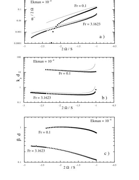
Figure 6: Maximal growth rate (2a), corresponding vertical wavenumber (2b) and azimuthal wavenumber (2c) as a function of the rotation number $2\Omega/S$ at $Ek=10^{-4}$, $Pr=\infty$ and for different stratifications. The line is the result of Molemaker et al. (2001), obtained at $Ek=0$.

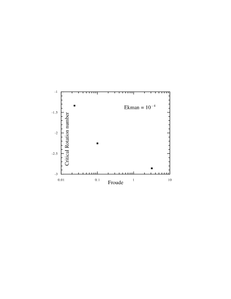
Figure 7: Critical rotation number vs. Froude number $(\Omega/N)$, at $Ek=10^{-4}$.

In Fig 8, we show the optimal growth rate and wavenumbers as functions of stratification, at $Ro=-4/3$, for different values of $Ek$. For comparison, the results obtained by Molemaker et al (2001) at $Ro=-3/2$ and $Ek=0$ (for different boundary condition!) are also displayed. The growth rate tends to be proportional to $N$ for large Froude numbers, but becomes a fraction of the dynamical frequency $\Omega$ for $Fr>1$. One sees that the viscosity (and boundary conditions) has little influence on the vertical wavenumber, which scales as $1/Fr$, while it introduces a sharp cut-off at small Froude numbers in both $\omega_{i}$ and $\beta$. This cut-off is pushed towards larger stratification with increasing viscosity. The cut-off defines a viscosity-dependent critical Froude number, below which no instability is present. Its dependence on the Reynolds number is approximately a power law $Fr_{c}\sim Re^{-1/2}$, as shown in Fig. 9.

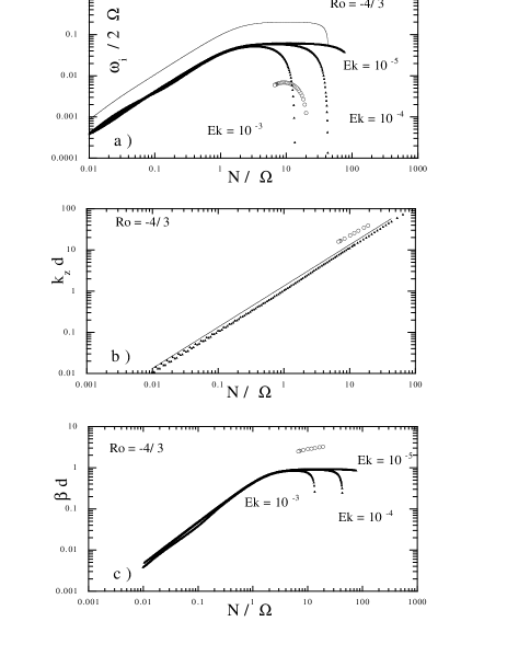
Figure 8: Maximal growth rate (4a), corresponding vertical wavenumber (4b) and azimuthal wavenumber (4c) as a function of the inverse Froude number at $Ro=-4/3$, $Pr=\infty$ and for different viscosity. The filled symbols correspond to the optimal eigen mode; the open symbols correspond to a member of the “large $\beta$ family”, computed at $Ek=10^{-5}$. The lines refer to the theoretical formulae proposed by Molemaker et al. (2001) for the optimal mode: $\omega_{i}/2\Omega=\beta de^{2Ro}$ and $k_{z}d=Ro/2Fr\sqrt{1+Ro}$.

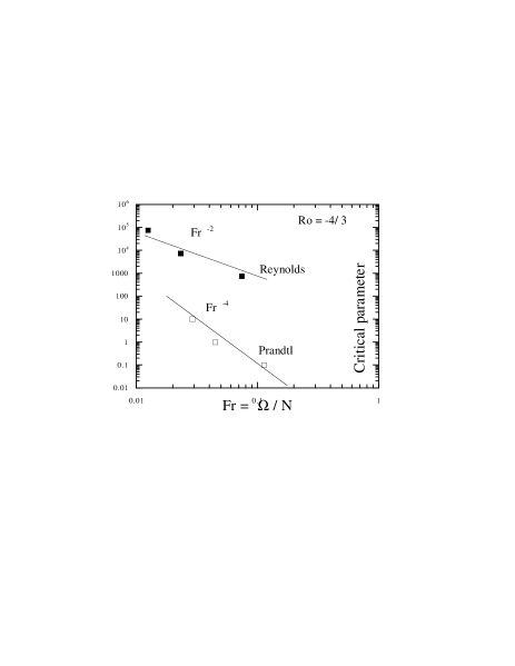
Figure 9: Variation of Reynolds and Prandtl numbers on the neutral stability lines at $Ro=-4/3$ as a function of the Froude number.

The variation with stratification indicates that at small stratification, the growth rate is proportional to $N$, while at large stratification, it is proportional to $\Omega$, i.e. independent of the stratification.

4.4 Influence of Prandtl number

For finite Prandtl number, the stratification agent (for example the temperature) undergoes a diffusive process, which can have a stabilizing influence. To study this effect, we fix $Ro=-4/3$ and $Ek=10^{-4}$, and decrease the Prandtl number from $Pr=\infty$ to $Pr=0.1$. The resulting optimal growth rate and wavenumbers are shown in Fig. 10. One sees that decreasing the Prandtl number at fixed Ekman number provides qualitatively the same effects as when increasing the Ekman number (previous Section): as $Pr$ is decreased, the critical Froude number is shifted towards higher values. We have checked that this similarity of behavior also extends to optimal wavenumbers: no incidence on vertical wavenumber, varying cut-off for $\beta$. The variation of the critical Froude number with Prandtl number is shown in Fig. 9. The variation of $Fr_{c}$ with $Pr$ is less steep than for $Re$, namely $Fr_{c}\sim Pr^{-1/4}$.

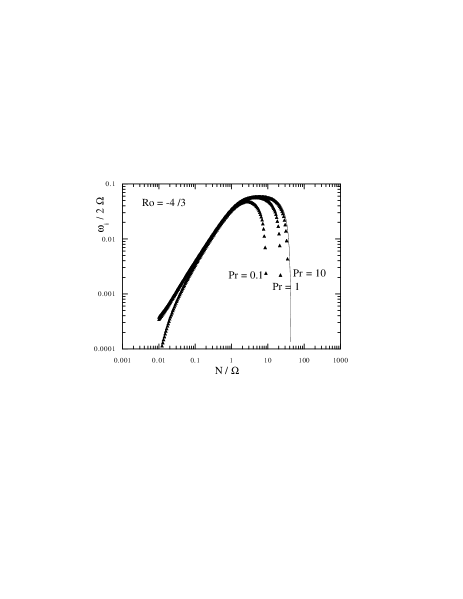
Figure 10: Maximal growth rate as a function of the inverse Froude number at $Ro=-4/3$, $Ek=10^{-4}$ and for different Prandtl numbers. The line is the result at $Pr=\infty$, drawn for comparison.

For illustration we also display in Fig. 11 a typical eigenmode solution for the radial velocity and entropy perturbation for $Ro=-4/3$, $Ek=10^{-4}$, $Fr=0.5$ and two values of the Prandtl number. One sees that these eigenfunctions vary smoothly over the channel width and that the change with Prandtl number is rather smooth and unimportant.

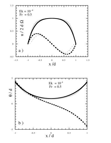
Figure 11: Real (continuous line) and imaginary (dotted line) part of the optimal eigenfunction for the radial velocity $u$ (Fig 7a) and for the scaled entropy fluctuation $\theta$ (Fig 7b), as a function of the $x$-coordinate, at $Ro=-4/3$, $Fr=0.5$, $Ek=10^{-4}$, and for $Pr=0.1$ (thin line) and 10 (thick line).

4.5 Influence of azimuthal wavenumber

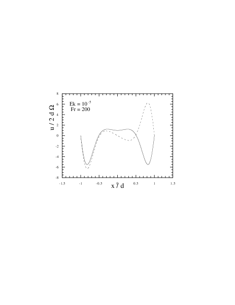
Figure 12: Real (continuous line) and imaginary (dotted line) part of a ”large $\beta$” eigenfunction for the radial velocity $u$, as a function of the $x$-coordinate, at $Ro=-4/3$ $Fr=200$ $Ek=10^{-5}$, $\beta d=3.3$, $k_{z}d=41$, $\omega_{i}/2\Omega=0.0013$ and for infinite Prandtl number.

Up to now, we have focused only on optimal modes (those with highest growthrate). These modes are characterized by a low azimuthal wavenumber. In the application to astrophysical disks, it may be interesting to look for modes with larger azimuthal wavenumber, which may be more realistic for very thin disks (for which $\beta d\sim r/H\gg 1$). Finding such modes is very time consuming using our numerical procedure (which is optimized for the detection of optimal growth rate). So, we focused on the case $Ro=-4/3$ and only explored the case $Ek=10^{-5}$, $Pr=\infty$. In that case, we were able to capture one member of the large $\beta$ family whose characteristics are shown in Fig. 8 for easier comparison with the optimal mode. The azimuthal and vertical wavenumber of this mode are roughly twice those of the optimal family. Its growth rate is about 10 times smaller. The corresponding velocity profile shows a double oscillation within the channel, see Fig. 12. The mode seems to exist only at rather large stratification $Fr>1$. All these features are reminiscent of the “large $\beta$ mode” found in the Taylor-Couette configuration by Molemaker et al. (2001). These modes are characterized by a “radial” wave number $k>2$, thereby producing $k$ oscillations of the eigenmode in the radial direction. The wavenumber roughly follows $k^{2}=\beta^{2}k_{z}^{2}$. Their growth rate, in the inviscid limit, scales as $|\Omega|k^{-1/4}e^{3Ro}$. With $k=2$, this gives $\omega_{i}/2\Omega=0.008$ in rather good agreement with our finding. This strongly suggests that these “large $\beta$ -modes” also exist in the plane Couette case. Since their growthrate is still a significant fraction of the rotation period, these modes are probably also quite relevant for astrophysical disks.

4.6 Comparison with experiments

It is interesting to compare our results with experimental data obtained in the same conditions (small gap limit) by Boubnov and Hopfinger (1995). We note that in this experiment the boundary conditions are probably rigid (in contrast with our numerical analysis). This comparison can then be used to probe the influence of boundary conditions. A difficulty arises because the experiments only provide data on the critical line, on which $Ro$, $Fr$ and $Re$ vary simultaneously. We thus analyze the three possible planes, in Fig. 13. In panel a), we observe a confirmation of the stabilizing role played by stratification: weak stratification tends to increase the range of instability, while large stratification (small Froude number) tends to restrict the domain of instability. The experimental points do not overlap with our numerical points, since the latter are performed at constant, and slightly sma ller Ekman number. In panel b), we do not observe any clear dependence of the rotation number on Reynolds number (different instability branches may be present). At $Ro=-4/3$, the Keplerian value, the critical Reynolds number seems to be between $4000$ and $10^{4}$, well below typical Reynolds number of e.g. circumstellar disks (Hersant et al, 2003). In panel c) one sees the dependence of the critical Reynolds number as a function of the stratification. At small Froude numbers, the experimental data seem to confirm the $Fr^{-2}$ scaling obtained numerically. At large Froude number, we observe another, linear scaling, of the Reynolds number with the Froude number, $Re_{c}\sim 2000Fr$. This number will be used below in our discussion.

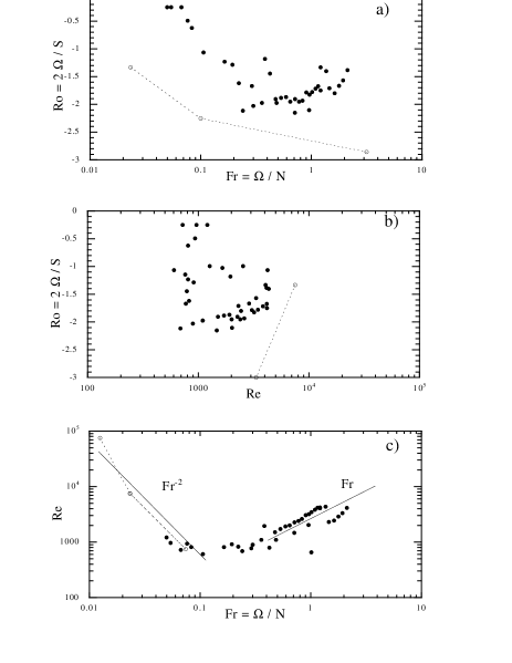
Figure 13: Neutral-stability curves ($\omega_{i}=0$) in the stratified Taylor-Couette flow experiment of Boubnov and Hopfinger (1995) in the small gap limit, in parameter space; a): in the plane $Ro,Fr$; b) in the plane $Ro,Re$; c) in the plane $Re,Fr$. The filled circles are the experimental data. The open circles are the numerical data obtained in the present paper.

5 Application to astrophysics

5.1 Stratification in disks

In previous Sections, we have shown that all flows with $S/2\Omega<0$ are linearly unstable with respect to non-axisymmetric perturbations in the presence of vertical stable stratification.

To decide whether an astrophysical disk is stably stratified, on has to solve for the vertical structure of the disk, which itself depends on how turbulent kinetic energy is transformed into heat through viscous friction. Most prescriptions for this heat release lead to stable stratifications.

One exception may be the central part of disks around black holes, where radiation pressure exceeds gas pressure, and where for this reason entropy decreases with distance from the equatorial plane, triggering thermal convection (Bisnovatyi-Kogan & Blinnikov 1977). But this does not take into account the illumination of the disk by hard X-rays, which is observed. The presence of thermal convection has also been suggested in disks around young stellar objects (Lin & Papaloizou 1980). However, here again a natural process leading to stable vertical stratification is the disk illumination by the central object (Chiang & Goldreich 1997).

A rough estimate of the Brunt-Väisälä frequency in stably stratified disks may be obtained in the thin disk approximation:

$$N^{2}={g\over H_{P}}\left[\nabla_{\rm ad}-\nabla\right]=\Omega^{2}\left({z\over H}\right)^{2}\left[\nabla_{\rm ad}-\nabla\right]$$ (53)

where the actual temperature gradient $d\ln T/d\ln P$ is determined by the opacity law; the adiabatic gradient $\nabla_{\rm ad}=(\partial\ln T/\partial\ln P)_{\rm ad}$ takes the value 0.4 for perfect atomic or ionized gas. Typically $[\nabla_{\rm ad}-\nabla]\approx 0.1$, and thus $N/\Omega\sim 0.3$. This value is confirmed by detailed calculations.

Radiative numerical simulations of protostellar disk (D’Alessio et al. 1998) reveal that at $r=0.5$ a.u. the temperature is of the order of $1000K$ at the disk scale height and $300K$ in the midplane, leading to $N/\Omega\sim 0.3$. In this regime, the critical Reynolds number is of the order of $1000$, the growthrate is about one percent of the rotation frequency and the typical vertical and azimuthal wavenumbers are about $0.1/d$. The largest allowed $d$ in this case is $0.1H$ leading to vertical scale and azimuthal wavenumber of the order of unity. The typical instability should then take the form of a spiral mode.

We can thus conclude that, in astrophysical disks, stable stratification is the rule rather than the exception. If this were not the case, one would invoke thermal convection as the obvious cause for the turbulence which ensures the accretion on the central object.

5.2 Magnetic field vs. stratification

Our findings are reminiscent of what occurs in the presence of an axial magnetic field. It is therefore interesting to examine the degree of similarity between the two instability mechanisms using the same tools. For this, we recall the results obtained by Chandrasekhar (1960). First, unlike the hydrodynamical instability in stratified disks, the magneto-rotational instability has axisymmetric unstable modes. For these modes, the sufficient stability condition is:

$$S/2\Omega>-\frac{1}{4}\frac{I_{1}}{k_{z}^{2}I_{0}}\frac{\Omega_{A}^{2}}{\Omega^{2}},\quad\rm{STABILITY}$$ (54)

where $\Omega_{A}=\sqrt{k_{z}^{2}\mu B_{z}^{2}/4\pi\rho}$ is the Alfvèn frequency. Comparing this condition with (13), we see strong similarities with the stratified case, the Brunt-Väissälä frequency being just replaced by the Alfvèn frequency. For example, strong magnetic fields tend to inhibit instability, in the same way as strong stratification, whereas in the limit of the weak magnetic field $S/2\Omega>0$ is a condition for stability, as for stratified, rotating shear flows. Keplerian flows, having $S/2\Omega=-3/4$ do not satisfy this stability criterion, and are therefore liable to both type of instabilities.

In a recent detailed numerical study of the magneto-rotational instability, Willis and Barenghi (2002) found that the critical Reynolds number at infinite Prandtl number is of the order of 20, that is one order of magnitude less than for the strato-rotational instability discussed here. They also noted that the variation of the critical Reynolds number with magnetic Prandtl number is $Re_{c}\sim 100/\sqrt{P_{m}}$, similar to the law found in Fig. 5 for stratification. However, in a typical disk, the magnetic Prandtl number is much lower than the Prandtl number. For example, in a protoplanetary disk, it is less than $10^{-5}$ (Rüdiger & Zhang 2001). This means that a typical critical Reynolds number for the magneto-rotational instability will be greater than $30000$, hence larger than the critical Reynolds number for strato-rotational instability.

5.3 Barotropic vs baroclinic instability?

In the present paper, we only focused on perturbations with typical radial scale small compared to the vertical scale height, leading to a barotropic description. An opposite limit would be to consider perturbations with small vertical scale, leading to a situation where only the vertical dependence is considered so that $\Omega$ varies with the axial coordinate $z$. In this situation, one may expect new instabilities to arise, due to the vertical shear. More generally, when the rotation departs from cylindrical, it may induce an axisymmetric baroclinic instability which has been described earlier in stellar interiors by Goldreich and Schubert (1967) and Fricke (1968). The application of this instability to disks has been recently done by Urpin (2003), who showed that the instability is linear, and that it proceeds on a thermal time-scale. More generally, baroclinic instabilities occur when there is an inclination between the density and pressure term, breaking the vorticity conservation. As discussed by Klahr and Bodenheimer (2003), this effect is likely to occur in any realistic disk. This means that in general, astrophysical disks are subject to both barotropic (as shown in this paper) and baroclinic instabilities. The interplay between these two instabilities is a fascinating subject, and has been widely studied in the oceanographic context. For upwelling flows it was found for example that barotropic instabilities are important in the early stages of the dynamics, while baroclinic modes dominate the late stages. The growthrate and wavenumbers are in between the growthrate and wavenumber of each instability (Tadepalli & Fertziger 1998). Clearly, a similar study would be welcome in the astrophysical context.

6 Conclusion

In this paper, we have used analytical and numerical methods to study the instability of Keplerian-like flow in the presence of a stable vertical stratification, for perturbations obeying rigid, stress-free or periodic boundary conditions in the radial coordinates that lie less than one scale height apart so as to justify an incompressibility approximation. This instability is non-axisymmetric. Its growth-rate is a fraction of the rotation rate at small stratification. This ‘strato-rotational’ instability is purely hydrodynamical and does not require the presence of any magnetic field, whatever small. Therefore, it is especially relevant in the context of weakly ionized disks, such as the primitive solar nebula. It is of course also relevant in other Keplerian disks, since the critical Reynolds number to trigger this instability is of the order of $10^{3}$, which is less than the critical Reynolds number for both the magneto-rotational instability and the finite-amplitude hydrodynamic instability. It may also interplay with baroclinic instabilities, resulting in mixed instabilities similar to those observed in oceans. However the question of which instability occurs first has little relevance, partly because we do not know the initial conditions, but mainly because there is no reason why the instability which has the fastest linear growth will dominate in the fully nonlinear state. What one should rather ask is what kind of turbulence exists at the high Reynolds numbers which characterize astrophysical disks. A partial answer to this question may already be found from Taylor-Couette laboratory measurements (Dubrulle et al. 2004), which provide information about the hydrodynamical regime of rotating shear flow, as well as the influence of magnetic field or stratification on the transport properties. When applied to circumstellar disks, this provides parameter free-predictions about accretion rates and fluctuations which are in good agreement with observations (Hersant et al. 2003). For the influence of processes more specific to astrophysics (radiative transport, etc.) one will probably have to wait until the numerical simulations are able to reach Reynolds numbers of order $10^{6}$ or more.

- (1) Balbus, S. A., Hawley, J. F. 1991, ApJ 376, 214
- (2) Bender, C. and Orszag, S. A., 1987, Advanced Mathematical Methods for Scientists Ad Engineers, Mc Graw Hill
- (3) Boubnov, B. M. and Hopfinger, E. 1997, Physics-Doklady 42, 312
- (4) Cambon, C., Benoit, J.-P., Shao, K. and Jacquin, L. 1994, J. Fluid Mech. 278, 175
- (5) Chandrasekhar, S. 1960, Proc. Nat. Acad. Sci. 46, 53
- (6) Chiang, E. I. and Goldreich, P. 1997, ApJ 490, 368
- (7) D’Alessio, P., Canto, J., Calvet, N. and Lizano, S. 1998, ApJ 500, 411
- (8) Dauchot, O. and Daviaud, F. 1994, Phys. Fluids 7, 335
- (9) Dauchot, O. and Manneville, P. 1997, J. Phys. II 7, 371
- (10) Dubrulle, B. and Knobloch, E. 1992, A&A 256, 673
- (11) Dubrulle, B. 1993, Icarus 106, 59
- (12) Dubrulle, B. and Graner, F. 1994, A&A 282, 277
- (13) Dubrulle, B., Dauchot, O., Daviaud, F., Longaretti, P.-Y., Richard, D. and Zahn, J.-P. 2004, submitted to Phys. Fluids (2004).
- (14) Fricke, K. 1968, Z. Astroph. 68, 317
- (15) Glatzel, W. 1987, MNRAS 225, 227
- (16) Goldreich, P. and Lynden-Bell, D. 1965, MNRAS, 130, 125
- (17) Goldreich, P. and Narayan, R. 1985, MNRAS 213, 7p
- (18) Goldreich, P. and Schubert, G. 1967, ApJ 150, 571
- (19) Kelvin, W 1887, Phil. Mag. 24(5), 89.
- (20) Hersant, F., Dubrulle, B. and Huré, J.-M. 2004 (to appear in A& A)
- (21) Klahr H. H. and Bodenheimer, P. 2003, ApJ 582, 869
- (22) Knobloch, E. Astrophys. 1985, Space Sciences 116, 159
- (23) Knobloch, E. 1996, Phys. Fluids 8, 1446
- (24) Korycansky, D. G. 1992, ApJ 399, 176
- (25) Kushner, P. J., McIntyre, M. E. and Sheperd, T. G. J. 1998, Phys. Oceanogr. 28, 513
- (26) Ioannou, P. J., and Kakouris, A. 2001, ApJ 550, 931
- (27) Lezius, D. K. and Johnston, J. P. 1971, Report MD-29 Thermoscience Division, Dept. Mech. Engineering, Stanford University
- (28) Lin, D. N. C. & Papaloizou, J. 1980, MNRAS 191, 37
- (29) Molemaker, M. J., McWilliams, J. C. and Yavneh, I. 2001, Phy. Rev. Letters 86, 5273
- (30) Nayfeh, A. 1978, Perturbations Methods, Wiley Ed.
- (31) Papaloizou, J. C. B. and Pringle, J. E. 1984, MNRAS 208, 721
- (32) Papaloizou, J. C. B. and Pringle, J. E. 1985, MNRAS 213, 799
- (33) Richard, D., “Instabilités Hydrodynamiques dans les Ecoulements en Rotation Différentielle”, 2001, Thèse de l’Université Paris 7
- (34) Richard, D. and Zahn, J.-P. 1999, A&A 347, 734
- (35) Rudiger, G. and Zhang, Y. 2001, A&A 378, 302
- (36) Snyder, H. A. 1968, Phys. Fluid 11, 728
- (37) Taylor, G. I. 1936, Proc. Roy. Soc. London A 157, 546
- (38) Velikhov, E. 1959, Soviet Phys. JETP 36, 1398
- (39) Urpin, V. 2003, A&A 408, 397
- (40) Wendt, F. 1933, Ing. Arch. 4, 577
- (41) Willis, A. P. and Barenghi, C. F. 2002, A&A 388, 688
- (42) Withjack, E. M., Chen, C. F. 1974, J. Fluid Mech. 66, 725.
- (43) Yavneh, I., McWilliams, J. C. and Molemaker, M. J. 2001, J. Fluid Mech. 448, 1