Comparing spectroscopic and photometric stellar mass estimates

Abstract

The purpose of this letter is to check the quality of different methods for estimating stellar masses of galaxies. We compare the results of (a) fitting stellar population synthesis models to broad band colors from SDSS and 2MASS, (b) the analysis of spectroscopic features of SDSS galaxies (Kauffmann et al., 2003), and, (c) a simple dynamical mass estimate based on SDSS velocity dispersions and effective radii. Knowing that all three methods can have significant biases, a comparison can help to establish their (relative) reliability. In this way, one can also probe the quality of the observationally cheap broadband color mass estimators for galaxies at higher redshift. Generally, masses based on broad-band colors and spectroscopic features agree reasonably well, with a rms scatter of only $\sim 0.2$ dex over almost 4 decades in mass. However, as may be expected, systematic differences do exist and have an amplitude of $\sim 0.15$ dex, corrleting with H$\alpha$ emission strength. Interestingly, masses from broad-band color fitting are in better agreement with dynamical masses than masses based on the analysis of spectroscopic features. In addition, the differences between the latter and the dynamical masses correlate with H$\alpha$ equivalent width, while this much less the case for the broad-band masses. We conclude that broad band color mass estimators, provided they are based on a large enough wavelength coverage and use an appropriate range of ages, metallicities and dust extinctions, can yield fairly reliable stellar masses for galaxies. This is a very encouraging result as such mass estimates are very likely the only ones available at significant redshifts for some time to come.

1 Introduction

The stellar mass of galaxies at the present epoch and the build-up of stellar mass over cosmic time has become the focus of intense research in the past few years.

In the local universe, results on the stellar mass function of galaxies were published using the new generation of wide-angle surveys in the optical (Sloan Digital Sky Survey; SDSS, York et al., 2000; 2dF, e.g. Folkes et al., 1999) and near-infrared (Two Micron All Sky Survey; 2MASS, Skrutskie et al., 1997). Cole et al. (2001) combined data from 2MASS and 2dF to derive the local stellar mass function, Bell et al. (2003) used the SDSS and 2MASS to the same end.

At $z>0$, a number of authors studied the stellar mass density as a function of redshift (Brinchmann & Ellis, 2000; Drory et al., 2001; Cohen, 2002; Dickinson et al., 2003; Fontana et al., 2003; Rudnick et al., 2003) reaching $z\sim 3$, while others, using wider field surveys, investigated the evolution of the mass function of galaxies (Drory et al., 2004; Fontana et al., 2004) to $z\sim 1.5$.

Generally, the high-redshift work relies on fits of multi-color photometry to a grid of composite stellar population (CSP) models to determine a stellar mass-to-light ratio, since large and complete spectroscopic samples of galaxies are not yet available. A similar approach was chosen by Cole et al. (2001) and Bell et al. (2003), too, at $z\sim 0$.

Taking advantage of the availability of photometry and spectroscopy for galaxies in the SDSS, Kauffmann et al. (2003, K03 hereafter) utilized spectroscopic diagnostics (4000Å Break, D_n4000, and the H$\delta_{\mathrm{A}}$ Balmer absorption line index ) to estimate the mean stellar age and the fraction of stars formed in recent bursts in each galaxy. By comparison of the colors predicted by their best-fit model to the object’s broad-band photometry they determine the amount of extinction by dust and hence the stellar mass-to-light ratio.

The purpose of this letter is to compare the stellar masses determined by this spectroscopic technique to masses obtained from multi-passband photometry and to compare both methods to a simple dynamical estimate of mass. Knowing that none of these methods yields a fiducial (stellar) mass, a comparison helps to establish the (relative) reliability of each method and makes us aware of potential differences between these estimators. Moreover, it can show us whether one can use observationally cheaper estimators as surrogates for more expensive (or unobtainable) ones, which is particularly important when dealing with high-redshift datasets.

Specifically, we want to know how the two estimators compare to each other, if using K-band $M/L$ yields better masses than using the g-band $M/L$ which is accessible at high $z$, and how these compare to a simple dynamical mass estimator, $M\sim\sigma^{2}R_{e}/G$.

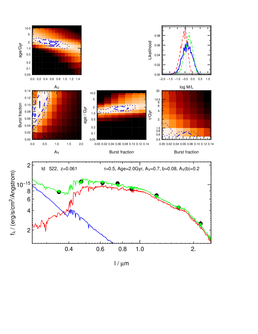
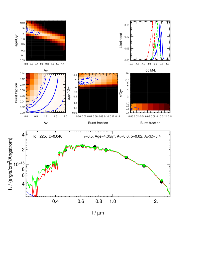
Figure 1: Illustration of the model-fitting technique used to estimate stellar masses. The lower panels show the comparison of the best fitting model to the photometric data. The red and blue lines represent the main and burst component, respectively. The green line represents the combined SED. The left hand side shows a young object with a burst component, the right side an older object. The upper panels show projections of the likelihood function onto four planes, age vs. dust in the main component, burst fraction vs. burst extinction, age of the main component vs. burst fraction, and star formation timescale, $\tau$, vs. burst fraction. The resulting likelihood distributions of $M/L$ are shown in the upper right panel on each side ($M/L_{g}$ blue; $M/L_{i}$ green; $M/L_{K}$ red). The $M/L$ of the best fitting model is indicated by vertical lines.

This letter is laid out as follows. In Sect. 2 we describe the sample of galaxies we use in this work. In Sect. 3 we give a brief overview of how we derive stellar masses by fitting CSP models to multi-band photometry. In Sect. 4 we compare these masses to the values in K03 and in Sect. 5 to a simple dynamical estimate of mass based on the SDSS velocity dispersions. We also discuss the implications of these comparisons.

We assume $\Omega_{\mathrm{M}}=0.3$, $\Omega_{\Lambda}=0.7$, and $H_{0}=70~{}\mathrm{km\ s^{-1}\ Mpc^{-1}}$ throughout this work.

2 The galaxy sample

The sample of galaxies we use in this work is selected from the NYU Value-Added Galaxy Catalog (Blanton et al., 2004). This is a merged catalog of objects from the SDSS Data Release Two (DR2) and 2MASS point-source and extended-source catalogs (and other catalogs which are not relevant here, as well).

We select all objects classified as galaxies and having a secure redshift measurement in the SDSS and that are detected in the 2MASS catalogs. From this set we randomly sub-select 20% of the objects leaving us with a sample of sample of $\sim 17000$ objects having redshifts and photometry in ugrizJHK.

We cross-correlate this catalog with the data from K03 to obtain their stellar mass estimates.

The galaxies in the sample span the absolute magnitude range $-15.3<M_{g}<-23.5$, the restframe $u\!-\!g$ color range $0.5<u\!-\!g<2.0$, and the (stellar) mass range $8<\log M<12$.

3 Deriving stellar masses

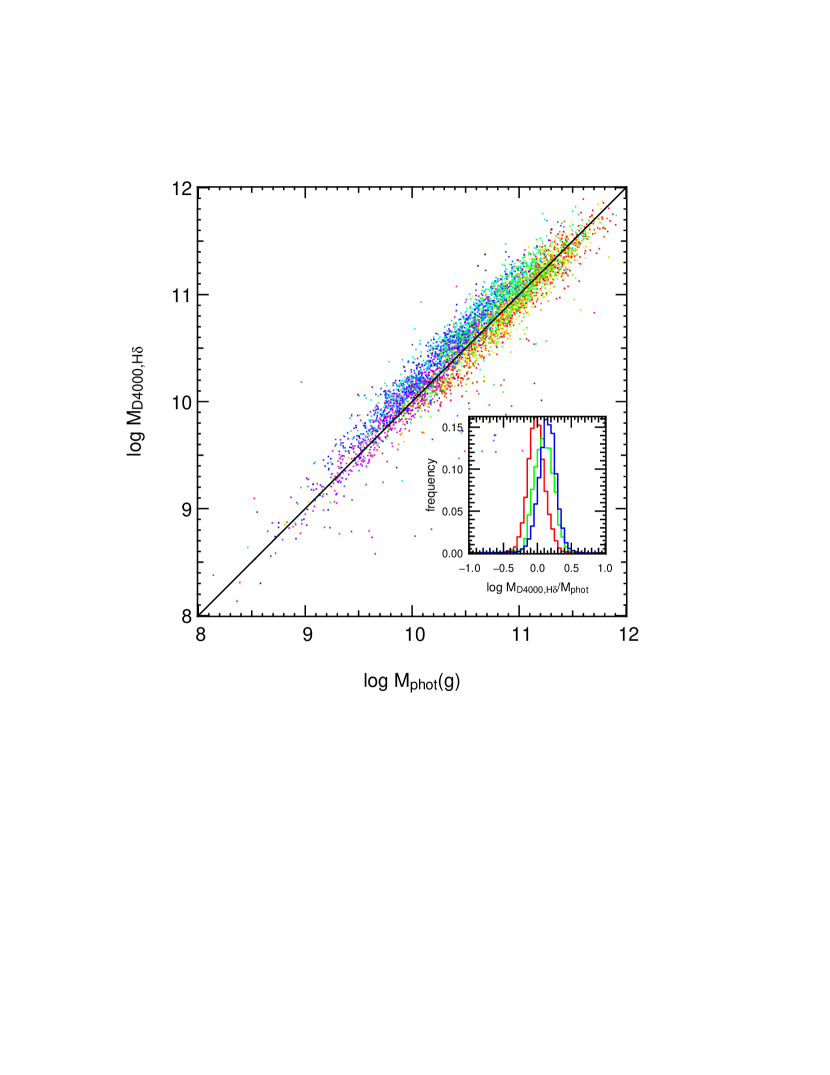
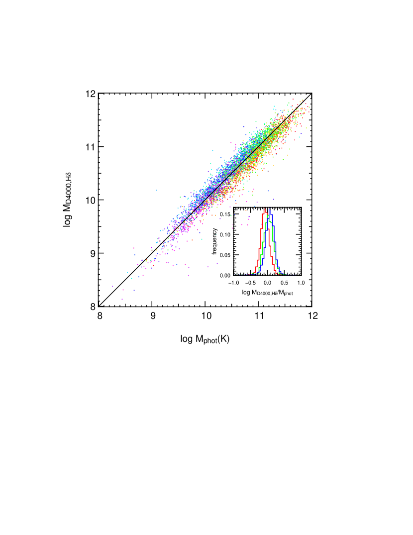
Figure 2: Comparison of our photometry-based stellar mass estimates to the stellar masses of K03. The left panel shows the masses of K03 plotted against our estimate based on $M/L_{g}$, the right hand panel against masses based on $M/L_{K}$. The colors denote H$\alpha$ equivalent width from no emission (red) to strong emission ($>25$Å; purple). The small panels show histograms of the residuals again as a function of H$\alpha$ equivalent width.

The method we use to infer stellar masses from multi-color photometry is an advancement of the program used in Drory et al. (2004). It is based on the comparison of multi-color photometry to a grid of stellar population synthesis models covering a wide range in parameters, especially star formation histories (SFHs).

We base our new model grid on the Bruzual & Charlot (2003) stellar population synthesis package. We parameterize the possible SFHs by a two-component model, consisting of a main component with a smooth analytically described SFH and a burst of star formation. The main component is parameterized by a star formation rate of the form $\psi(t)\propto\exp(-t/\tau)$, with $\tau\in[0.1,\infty]$ Gyr and a metallicity of $-0.6<\mathrm{[Fe/H]}<0.3$. The age, $t$, is allowed to vary between 0.5 Gyr and the age of the universe (at the object’s redshift).

The smooth component is linearly combined with a burst of star formation, which is modeled as a 100 Myr old constant star formation rate episode of solar metallicity. We restrict the burst fraction, $\beta$, to the range $0<\beta<0.15$ in mass (higher values of $\beta$ are degenerate and unnecessary since this case is covered by models with a young main component). We adopt a Salpeter initial mass function for both components, with lower and upper mass cutoffs of 0.1 and 100 $\mathrm{M_{\odot}}$.

Additionally, both the main component and the burst are allowed to exhibit a variable amount of extinction by dust. This takes into account the fact that young stars are found in dusty environments and that the starlight from the galaxy as a whole may be reddened by a (geometry dependent) different amount. In fact, Stasińska et al. (2004) find that the extinction derived from the Balmer decrement in the SDSS sample is independent of inclination, which, on the other hand, is driving global extinction (Tully et al., 1998, see, e.g.,). This is different from the approach taken by K03, where a single extinction value for the whole galaxy is used.

We compute the full likelihood distribution on a grid in this 6-dimensional parameter space ($\tau,\mathrm{[Fe/H]},t,A_{V}^{1},\beta,A_{V}^{2}$), the likelihood of each model being $\propto\exp(-\chi^{2}/2)$. To compute the likelihood distribution of $M/L$, we weight the $M/L$ of each model by its likelihood and marginalize over all parameters. The uncertainty in $M/L$ is obtained from the width of this distribution.

This procedure is illustrated in Fig. 1, where we show SEDs and likelihood functions for two objects, a young object with a high burst fraction, and an older and fairly quiescent object. We show projections of the likelihood function onto four planes in parameter space, age vs. dust in the main component, burst fraction vs. burst extinction, age of the main component vs. burst fraction, and star formation timescale, $\tau$, vs. burst fraction. The figure also shows the resulting likelihood distributions of $M/L$ in the g, i, and K bands. Note that for the quiescent object, the width of the $M/L$ distribution is very similar in the g and K bands, while it is much wider in g than it is in K for the younger star forming object. On average, the width of the likelihood distribution of $M/L$ at 68% confidence level is between $\pm 0.1$ and $\pm 0.2$ dex (using $M/L_{g}$). The uncertainty in mass has a weak dependence on mass (increasing with lower $S/N$ photometry) and much of the variation is in spectral type: early-type galaxies have more tightly constrained masses than late types (see also Fig. 1). Using the U band, the uncertainty in mass grows by $\sim 0.05$ dex.

4 Comparison of stellar mass estimators

In Fig. 2 we compare our photometry-based stellar mass estimates to the stellar masses of K03. We show the H$\alpha$ equivalent width (as measured by the SDSS) by color coding. The overall impression from this figure is that the two different estimators agree remarkably well, within a rms scatter of only $\sim 0.2$ dex over almost 4 decades in mass (and hence they largely agree within their respective uncertainties). This is only a relative statement, though. It does not imply that the masses are accurate to that level in an absolute sense, although it is very reaffirming. However, as may be expected, there are systematic differences as a function of star formation activity on the $\sim 0.15$ dex level.

The D_n4000 and H$\delta_{\mathrm{A}}$ based method of K03 yields masses almost identical to ours for weakly star forming objects (EqW(H$\alpha$) $<5$Å) at masses above $10^{10.5}$ $\mathrm{M_{\odot}}$. At lower masses, our estimator tends to give slightly higher masses than K03’s. For more strongly star forming objects, the photometrically determined masses are smaller than the ones of K03. For objects with EqW(H$\alpha$) $>25$Å, the discrepancy becomes as large as 0.15 dex, independent of mass. Note that at high redshift, such objects will be more common.

We suspect that there are a multitude of reasons for these differences based on the different sampling of stellar populations by both methods (if we leave out the JHK bands, our masses become more similar in their trends to K03’s, although with increased scatter). Plausibly, though, this is explainable by the fact that the photometrically determined masses sample the light from the whole galaxy, while K03’s SDSS-based sampling of D_n4000 and H$\delta_{\mathrm{A}}$ covers only the inner 3 arcseconds. Since most galaxies are redder in their centers than in the outer parts, this might lead to higher masses for star forming disk galaxies. Early-type galaxies without blue star forming disks do not suffer from this effect. This is confirmed by restricting the sample to low redshifts, which maximizes the effect. Also, at the lowest masses, galaxies might have more irregular SFHs, and photometric methods might fail in this case (Bell & de Jong, 2001). However, Fig.2 does not show a dependence of the residuals on mass, only on current star formation rate.

Fig. 2 also shows that our masses based on the g band are very similar to the ones estimated through the K band. For early type systems and weakly star forming systems, they are statistically indistinguishable. Star forming systems, however, tend to have g-band masses lower by $\sim 0.1$ dex. The good agreement is partly due to the fact that the effect of dust extinction and age on the effective $M/L$ are very similar in canonical models, as has been pointed out by Bell & de Jong (2001), although they are not completely degenerate. Typically, the spread of the stellar $M/L$ in the galaxy population at any given luminosity is around 0.7 dex in g and 0.35 dex in K. These results is reaffirming since the restframe blue spectral range is accessible to photometry to very high redshift, and thus high-$z$ studies mostly rely on $M/L_{B}$.

5 Comparison with dynamical masses

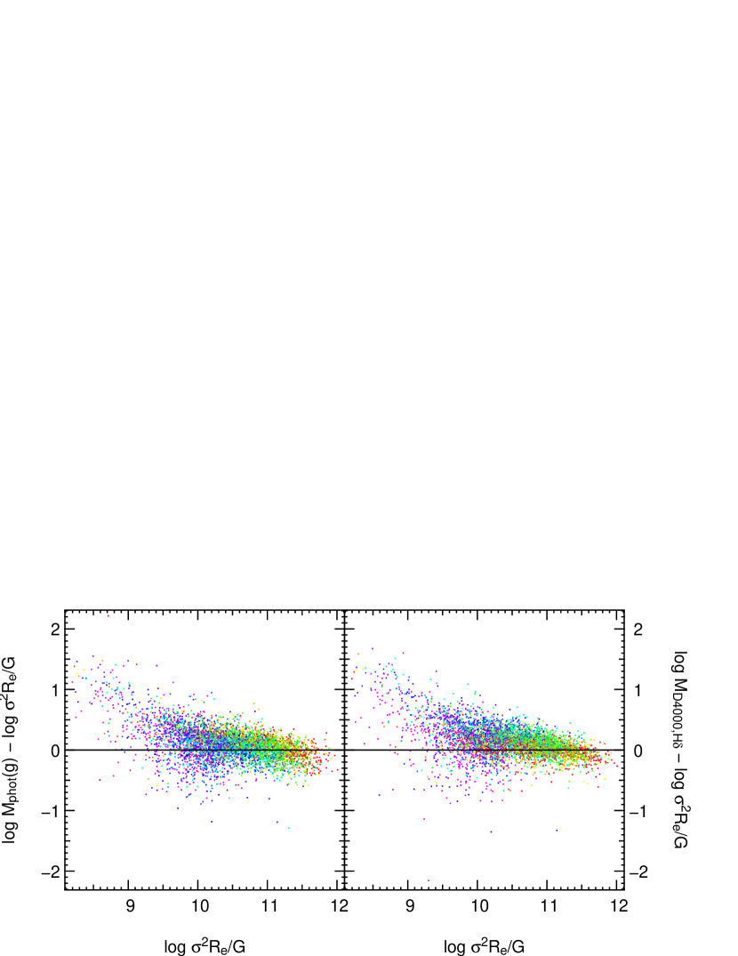
Figure 3: Comparison of stellar mass vs. dynamical mass, $M_{\mathrm{dyn}}\propto\sigma^{2}R_{e}/G$. The left hand panel shows $M_{\mathrm{dyn}}$ vs. photometric mass and the right hand panel shows $M_{\mathrm{dyn}}$ vs. the masses of K03. Color encodes H$\alpha$ equivalent width, as in Fig. 2.

Since we do not have a fiducial mass estimator (neither for stellar mass nor for total mass, for that matter), it is only natural to ask how the stellar mass measurements presented here compare with estimators of mass based on kinematic data. In fact, it has been suggested that stellar mass (or, more accurately, baryonic mass) and total mass are tightly related and that stellar mass can be used as a surrogate for total mass in the context of high-$z$ galaxy surveys to probe structure formation (see, e.g., Brinchmann & Ellis, 2000).

We use the measurements of velocity dispersion, $\sigma$, and effective radius in the g band, $R_{e}$, provided by the SDSS pipeline to plot stellar mass vs. dynamical mass, $M_{\mathrm{dyn}}\propto\sigma^{2}R_{e}/G$, in Fig. 3. The left hand panel shows $M_{\mathrm{dyn}}$ vs. photometric stellar mass and the right hand panel shows $M_{\mathrm{dyn}}$ vs. the stellar masses of K03. Color again encodes H$\alpha$ equivalent width.

Above $10^{10}$ $\mathrm{M_{\odot}}$, the stellar masses from both methods follow the dynamical masses remarkably well. Below $\sim 10^{9}$ $\mathrm{M_{\odot}}$, the velocity dispersion measurements of the SDSS becomes unreliable as we approach the instrumental resolution of the data ($\sim 70$ km s^-1).

At higher masses, although both estimators generally follow $M_{\mathrm{dyn}}$, there are again some differences, and both estimators show similar trends in their residuals although with different amplitudes. Stellar masses agree very well with $M_{\mathrm{dyn}}$ at the highest masses (which are mostly populated by old, quiescent objects). At lower masses, stellar masses show a trend to larger values than $M_{\mathrm{dyn}}$ with decreasing mass and with increasing H$\alpha$ emission line equivalent width. This effect is weak in the photometric estimator, and stronger in K03’s method, which gives stellar masses larger than $M_{\mathrm{dyn}}$ by 0.1 to 0.4 dex at almost all masses. This comparison is unchanged by using $M/L_{K}$ instead of $M/L_{g}$.

It is important to note that $M_{\mathrm{dyn}}$ is not a good estimator of total mass, and that this comparison is again only to be taken in relative terms. In fact $\sigma^{2}R_{e}/G$ can only provide a lower limit to the mass. However, as long as a bulge is present, the total mass should not be underestimated by more than $\sim 0.3$ dex (see, e.g. Fig. 4 in Whitmore & Kirshner, 1981; also Padmanabhan et al., 2004, who show that $\sigma^{2}R_{e}/G$ is a reasonable mass estimator, although this paper is concerned with ellipticals only). It is therefore not surprising to find stellar masses in excess of $M_{\mathrm{dyn}}$ and the difference between the two increasing at lower masses.

Nevertheless, the point of this work is to assess the general consistency and reliability of stellar mass estimates than to investigate the relationship between stellar and dynamical mass in galaxies. Fig. 3 shows that the estimators of stellar mass, and especially the photometric estimator which is most easily obtainable for large high redshift samples (covering a bluer wavelength range, though), closely follow $M_{\mathrm{dyn}}$ as measured by this simple dynamical measure. We cannot see significant systematic deviations which would bias or invalidate this estimator. This is a very encouraging result, since such an estimator is very likely to be the only one available at $z>0$ for some time to come.

References

- Bell & de Jong (2001) Bell, E. F., & de Jong, R. S. 2001, ApJ, 550, 212
- Bell et al. (2003) Bell, E. F., McIntosh, D. H., Katz, N., & Weinberg, M. D. 2003, ApJ, submitted
- Blanton et al. (2004) Blanton, M. R., Schlegel, D. J., & Hogg, D. W., in prep.
- Brinchmann & Ellis (2000) Brinchmann, J., & Ellis, R. S. 2000, ApJ, 536, L77
- Bruzual & Charlot (2003) Bruzual, G., & Charlot, S. 2003, MNRAS, 344, 1000
- Cohen (2002) Cohen, J. G. 2002, ApJ, 567, 672
- Cole et al. (2001) Cole, S., et al. 2001, MNRAS, 326, 255
- Dickinson et al. (2003) Dickinson, M., Papovich, C., Ferguson, H. C., & Budavári, T. 2003, ApJ, 587, 25
- Drory et al. (2004) Drory, N., Bender, R., Feulner, G., Hopp, U., Maraston, C., Snigula, J., & Hill, G. J. 2004, ApJ, 608, 742
- Drory et al. (2001) Drory, N., Bender, R., Snigula, J., Feulner, G., Hopp, U., Maraston, C., Hill, G. J., & de Oliveira, C. M. 2001, ApJ, 562, L111
- Folkes et al. (1999) Folkes, S., et al. 1999, MNRAS, 308, 459
- Fontana et al. (2003) Fontana, A., et al. 2003, ApJ, 594, L9
- Fontana et al. (2004) Fontana, A., et al. 2004, A&A, in press
- Kauffmann et al. (2003) Kauffmann, G., et al. 2003, MNRAS, 341, 33
- Padmanabhan et al. (2004) Padmanabhan, N., et al. 2004, New Astronomy, 9, 329
- Rudnick et al. (2003) Rudnick, G., et al. 2003, ApJ, 599, 847
- Skrutskie et al. (1997) Skrutskie, M. F., et al. 1997, in ASSL Vol. 210: The Impact of Large Scale Near-IR Sky Surveys, 25
- Stasińska et al. (2004) Stasińska, G., Mateus, A., Sodré, L., & Szczerba, R. 2004, A&A, 420, 475
- Tully et al. (1998) Tully, R. B., Pierce, M. J., Huang, J., Saunders, W., Verheijen, M. A. W., & Witchalls, P. L. 1998, AJ, 115, 2264
- Whitmore & Kirshner (1981) Whitmore, B. C., & Kirshner, R. P. 1981, ApJ, 250, 43
- York et al. (2000) York, D. G., et al. 2000, AJ, 120, 1579