SZ cluster science with the Planck HFI experiment

Abstract

In the near future the Planck satellite [1] will gather impressive information about the anisotropies of the cosmic microwave background and about the galaxy clusters which perturb that signal. We will here review the ability of Planck to extract information about these galaxy clusters through the Sunyaev-Zeldovich imprint. We will conclude that Planck will provide a catalogue of galaxy clusters, which will be very useful for future targeted observations. We will explain why Planck will not be very good in extracting detailed information about individual clusters, except for the dominating Compton parameter, $y$, which will be measured to a few percent for individual clusters. In this last point I am being rather conservative, but that will leave space for pleasant surprises when the Planck data will be analysed.

1 Introduction

The Planck satellite will be a real piece of art and an amazing piece of hardware. It will provide us with information about the cosmic background radiation (CMB) beyond the wildest imagination of most people, surely beyond mine. The sensitive detector will be sent far into space, over a million kilometers from earth, where it will be better protected from the Sun and Earth radiation. The satellite will be spinning and carefully mapping the whole sky. Thus it will give us accurate data about the full CMB sky, and about all the obstructions and contaminations between us and the last scattering surface of the CMB.

Many research years have been, and will still be, devoted to the analysis and interpretation (and possibly even understanding) of the CMB signal, and there is no question that the main scientific goal of Planck will be to carefully study the CMB. In that sense all the foregrounds, such as galaxy clusters and dust, are just contaminations which will have to be carefully removed. I am going to be discussing if we can use this removed “contamination” for anything useful. It is rather amusing that such beautiful structures as galaxies and galaxy clusters are just considered to be contamination by many CMB people.

The analysis of the Planck CMB data will determine many of the cosmological parameters very accurately. This includes dark matter and dark energy parameters as described by R. Bean and A. Melchiorri in these proceedings. Numerous papers have reviewed the expected precision with which Planck will determine such parameters, including refs. [2, 3, 4].

One important strength of Planck is that it will have 9 observing frequencies, and as we will see below this will allow a separation of the CMB signal from the contaminations. The actual construction and optimization of performance of the Planck detector is a very complicated process, and I refer to the lectures by P. de Bernardis and J. M. Lamarre in these proceedings for all the details. There are also recent nice reviews on the two instruments on-board Planck [5, 6], see also [7, 8, 9].

Planck will find of the order 10 thousand massive galaxy clusters out to a redshift of $z\sim 1.5$. This cluster catalogue will be deeper and larger (all sky survey) than any other existing catalogue. This cluster catalogue will be very useful on its own and for future follow-up observations. It is the goal of this lecture to discuss at an elementary level how this will be achieved, and secondly we will discuss more carefully what Planck will not be able to do. Several groups have addressed similar issues already, see e.g. refs. [10, 11, 12].

2 Extracting the CMB

The first question we have to ask is naturally how bad are the contaminations? Or in other words, will we be able to extract the CMB signal accurately enough to do proper CMB parameter extraction?

There are many foreground components which will have to be removed, these include infrared galaxies, dust, synchrotron radiation, free-free emission, radio sources and the Sunyaev-Zeldovich effect. It turns out that the dominating contamination at the CMB frequencies is the SZ effect, and it is therefore crucial that we can separate the CMB signal from the SZ signal. We will discuss the physics of the SZ effect in the next section. As is clear from fig. 1 (from ref. [13], see also ref. [14]) the power spectrum of the CMB is dominated by the SZ effect for $l>2000$. This is very important for the CMB analyses of inflationary parameters, because if we wish to allow e.g. a variation of the spectral index, then a contamination free high-l part of the power spectrum is crucial [15].

Figure 1: The CMB power spectrum is seriously contaminated by the SZ power for $l>2000$. The first question is, if this poses a serious problem for CMB analysis? Figure taken from ref.[13].

Now, how is this component separation done? The different signals will have different frequency dependence. For instance, the unresolved radio sources will have most power at low frequencies (30-70 GHz), and the dust will have most power at high frequencies (545-857 GHz). Fortunately the SZ signal will be sitting right in the middle, with most power on frequencies 143-353 GHz. Thus, if we have several observing frequencies then we can use the different frequency dependence of the signals to separate them. For an excellent review of the different contaminations see [16]. As mentioned in the introduction, Planck will have 9 observing frequencies between $30$ and $857$ GHz. In this way Planck can very carefully separate all the different signals, hence removing the contaminations from the CMB signal. The frequencies important for SZ science, 143-353 GHz are sitting on the HFI instrument [6].

Already years ago it was understood that this component separation works so well that the SZ signal will not be a major obstruction to CMB science [17, 18], and this has been confirmed by several much more advanced studies [12, 19]. An early figure showing that the reconstructed CMB power is sufficiently accurate it presented in fig. 2

Figure 2: The dotted line is the true CMB signal, and the full line is the CMB signal plus non-removed SZ contamination. The CMB power is well recovered from the contaminated signal. Here the figure uses $k\approx 28\cdot l$, and the Power is the “plane” approximation of the normal $C_{l}$ (Fourier coefficients instead of spherical harmonics). Figure taken from ref. [18].

One point deserves a few comments, namely that the kinetic SZ effect has the same spectral behaviour as the CMB signal itself. How can one then separate these two? Basically one has to take advantage of the fact that the thermal and kinetic SZ effects are spatially correlated. Thus if you find a cluster (through the thermal effect) then you can expect a kinetic effect to be right at that point in space - and at that point only. You can therefore interpolate (guess) the surrounding CMB signal through those points, and then you are left with the kinetic effect [20]. This method seems to work surprisingly well.

We may summarize this section by stating that even though the SZ signal is very large, then it can be removed sufficiently accurately that the CMB analysis can be performed with no problem. This was the main goal of Planck, to do CMB analysis, so everyone is happy. The next question to ask is whether we can use the removed SZ signal itself for a further cluster analysis?

3 The Sunyaev-Zeldovich effect

Let us make a small break from Planck and briefly discuss the SZ effect itself.

Galaxy clusters typically have temperatures of the order keV, $T=1-10$ keV. Therefore a CMB photon which traverses the cluster and happens to Compton scatter off a hot electron will get increased momentum. This up-scattering of CMB photons, which results in a small change in the intensity of the cosmic microwave background, is known as the Sunyaev-Zeldovich effect, and was predicted just over 30 years ago [21]. The first radiometric observations came few years later [22, 23], and while recent years have seen an impressive improvement in observational techniques and sensitivity [24, 25], the near future observations will see another boost in sensitivity by orders of magnitude.

From a theory point of view, the importance of a correct treatment of the electron distribution function was emphasized about 25 years ago [26], but an exact calculation of the SZ effect was made only recently [27]. Numerous groups have considered expansion in temperature, which works accurately enough, and all the details are presented by Y. Rephaeli and N. Itoh in these proceedings, and in the references [28, 29, 30, 31].

In principle the relativistic corrections from a high electron temperature can be measured with a multi-frequency observation, and hence one can use purely the SZ effect to determine the cluster temperature [32, 33]. This method is complementary to X-ray observations, because the SZ temperature determination, which simultaneously measures the electron density, $n_{e}$, does not depend on an unknown clumping factor, as does the X-ray detection. Furthermore, the SZ effect depends on very simple physics, whereas understanding the X-ray signal is very complicated.

We have analysed existing SZ data and made the first cluster temperature detections using purely the SZ observations [33, 34]. These temperature detections have large error-bars due to the limited sensitivity of present day observations, but it has hereby been shown that this method of temperature determination works, and this method can become a powerful tool for cluster studies with future dedicated SZ surveys, and we will later ask how well Planck will do here.

4 Finding the clusters

Most clusters have angular size of about 2 arcmin, so since Planck channels will have angular resolution of 5 arcmin for 217 and 353 GHz channels (and 7 arcmin for 143 GHz), then the individual clusters will not be spatially resolved (except a few very nearby ones) [11]. Whatever characteristics of the cluster we are going to measure will be averaged over the full cluster. At some stage one will have to ask how this average is done, is it an average over mass, an average over X-ray intensity, or an average over SZ-intensity? Naturally there will be a difference between averages over X-ray or SZ intensity, and one should therefore be rather careful with this technical point [35].

A good way of thinking of the cluster detection is the following [11]. First you use all the very high and very low frequencies to remove foreground contamination. Next take the difference between the 353 GHz and the 217 GHz channels. These two channels have the same angular resolution, and since the SZ effect roughly vanishes at 217 GHZ, then the resulting map will be a fair representation of the clusters. That’s it! We now have a full sky map of all the clusters, which are simply sitting at the maxima of this difference-map. This method is really simplistic, and this is just a good way of thinking of the procedure.

Next you naturally have to start asking how well this procedure works. What is the completeness, that is how many of all the clusters did you actually find? Second, what is the reliability, that is how many non-existing clusters did you find? With these two numbers you get a good measure of your cluster detection algorithm, and one can start discussing which is the optimal. Today very advanced methods have been developed, see e.g. [36, 12, 37, 38, 39].

We should dwell a while on the question of completeness and reliability. In order to get these two important numbers we need a full test sky map of clusters. Basically we need to know what Planck realistically will be seeing, and since a numerical simulation of a full universe with both dark matter and baryons is impossible today (by far!), then we have to do something smarter.

First we have to get realistic clusters and peculiar velocities, and to that end we must make a full sky simulation of the dark matter structures [40]. Collisionless dark matter is relatively simple to simulate, so this will allow up to $10^{9}$ particles in the simulation. This will provide the basic structure of the entire universe, namely a description of the positions and peculiar velocities of all the gravitationally dominating dark matter.

Next you need to include the baryons. After all, the SZ effect is a measure of the distribution of the baryons and electrons, so this should be done as carefully as possible. For a given total mass of the dark matter structure we know fairly well the radial distribution of the dark matter [41, 42, 43]. Thus, you just need for ’each’ of the DM structures in the full universe simulation to make another simulation including the baryons. This is naturally impossible, so instead one makes the following smart trick. We simulate several clusters of different masses. In reality we only simulate relatively few, but we do those very carefully. Then for a given cluster from the full DM simulation we can ’interpolate’ between these accurately calculated clusters. This procedure is astounding, in my view, and the results are impressive! The most recent implementations [37, 12] thus provide a very realistic full SZ sky, both thermal and kinetic.

Let us get the perspective back. We now have a realistic full SZ sky, and we can use this to develop different methods of finding clusters. Even better, we can compare the methods and find which one is the best for Planck. The conclusion is roughly that Planck will detect about $10^{4}$ clusters out to redshift slightly beyond $z=1$, with fairly good completeness and reliability.

Thus Planck will create a beautiful catalogue of clusters, which basically includes all the massive clusters all the way out to redshift of 1 or $1.5$. This catalogue is larger, deeper and has more sky-coverage than any other existing catalogue. This cluster catalogue will be very useful for future follow-up observations. One can e.g. imagine a targeted SZ study, which selects the 100 brightest clusters in the universe for a careful study of radial temperature and density profile, which then can be compared with numerical simulations. We remember that the SZ observations are particularly powerful for large radii and for distant clusters. The last is because the SZ is a distortion of the CMB and hence basically redshift independent, and the ’large radius’ is because the SZ effect is proportional to the electron density, $I_{SZ}\sim n_{e}$, whereas the X-ray emission is proportional to the electron density squared, $S_{X}\sim n_{e}^{2}$. I wish to repeat and emphasize that this catalogue in itself is very useful, and we should do our best to make it as accurate as possible!

Now, having established that the catalogue will come into existence, let us proceed and discuss how accurately we will measure the cluster parameters of the individual clusters.

5 Cosmology from the cluster catalogue?

Basically, when we know the number, $n(M)$, of clusters of mass M, as a function of redshift z, then we know the cosmology. Thus if we have a complete and reliable catalogue which gives us $n(M)$, then we can extract cosmological parameters like the matter density, $\Omega_{M}$, cosmological constant, $\Omega_{\Lambda}$ etc etc (see e.g. [44] for references). I personally believe that most of the studies conducted so far (which I do not cite here) are very optimistic, and I do not advise people to blindly perform parameter extraction with the cluster catalogue. Some of the reasons are the following.

Figure 3: The dilution effect from the relativistic corrections. The solid line is the non-relativistic effect (cold cluster), and the dashed (dotted) line is for a 10 keV (20 keV) cluster. Figure taken from ref. [18].

The first point is naturally that one must understand the completeness and reliability of the catalogue very accurately, in order to get realistic error-bars. Many people have studied these numbers, however, there are always effects which are not included, and the systematic error-bars from non-included effects are very hard to estimate. For instance, the relativistic corrections to the SZ effect will dilute the SZ signal at 353 GHz, which implies that a given cluster will appear less bright than expected (see fig. 3). This will be a problem for the marginally detectable clusters; we may think we should see them, but because of the dilution effect they may be just non-detectable. Even worse, the dilution effect is largest for the large and bright clusters, which are very important for cosmological parameter extraction.

Another point is the question of scaling-relations. Basically we have to make an assumption about the connection between temperature and mass, the famous M-T relation. But what do we use here? Do we use the observed M-T relation from X-ray observations? No, because the weight from non-isothermal clusters is different between X-ray observations and SZ observations. Do we use a theoretical M-T relation or one from simulations? I think this would be very dangerous, after all these relations are still not in very good agreement with observations, even after years of effort. And finally, in most of these studies one has to make an assumption about the radial dependence of the baryons in the clusters, and what do we choose - A beta-model for the baryons [45], or a NFW profile [41], or something completely different [46, 47]? Basically my worry is, that it is unclear today how to realistically estimate the systematic error-bars from an insufficient (or incorrect) assumed profile.

Thus, I personally don’t believe we are in a position to use the Planck cluster catalogue for a measurement of cosmological parameters yet - there is still much work needed before we reach that level. I should clarify that all those objections above are my personal view, and that many scientists, even very good ones, believe that I am being overly pessimistic. However, this leaves space for pleasant surprises down the data-analysis road.

6 Cluster parameters from single clusters

Having read the section above you may be asking yourself: Why don’t we simply measure the cluster temperature of the individual clusters directly with the SZ? After all, the SZ effect depends on 3 parameter, the dominating Compton parameter $y$, the peculiar velocity, $v_{p}$, and the cluster temperature, $T_{e}$. If we have multi-frequency observation of the SZ effect, then we can separate the components and directly measure the cluster temperature.

Figure 4: Two clusters with different temperatures and peculiar velocity, $T=5$ keV, $v_{p}=-145$ km/sec and $T=7$ keV, $v_{p}=-260$ km/sec (full and dotted lines) are virtually indistinguishable, whereas the cluster with $T=6$ keV, $v_{p}=0$ km/sec (dashed line) is clearly different. Figure taken from ref. [48].

The first problem is that some of the cluster parameters are degenerate. This means that two clusters with different temperature, peculiar velocity and Compton parameter, may produce virtually indistinguishable spectra. An example hereof is given in fig. 4 where two clusters (full and dotted lines) have parameters, $T=5$ keV, $v_{p}=-145$ km/sec and $T=7$ keV, $v_{p}=-260$ km/sec respectively. These two lines are essentially on top of each other. In comparison, the cluster (dashed line) with $T=6$ keV, $v_{p}=0$ km/sec is clearly different.

Another problem is that the SZ signal is contaminated. The signal which we have to analyse is a sum of different components. First there is the SZ signal, but there is also interstellar dust emission, infra-red galaxies and radio sources. Naturally there is also a contamination from the CMB itself. All these contaminations have to be either monitored and removed, or controlled and extracted [49, 10, 50, 51, 52, 53, 54, 55, 56].

At the end of the day you will still be left with a little bit of contamination - it is simply not possible to remove everything. A specific example could be that you assumed that the non-removed radio sources (or the dusty galaxies) would have a specific spectral behaviour - e.g. a simple power-law. This may be a wrong assumption and you would systematically be biasing your results.

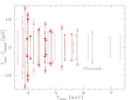
Figure 5: The temperature of individual clusters will have larger error-bars.

How would this affect the SZ parameters? Let’s assume that you have a little bit of non-removed radio sources. That means that you have removed most of the radio sources, but there is still a little bit you didn’t completely remove, maybe because you made the simplifying assumption that it follows a power-law. A contamination from radio sources gives a positive contribution at low frequencies, where the dominating $y$ parameter is determined, leading to a smaller value for $y$. Now, with this smaller value for $y$, the high frequency signal seems too high, which can only be compensated with a very small temperature. Finally, the velocity term goes like $v_{p}/T_{e}$, so with a very small temperature, $v_{p}$ is also forced to be very small. In reality, this leads approximately to $T_{e}\approx v_{p}\approx 0$.

Similarly, the effect on the SZ parameters from a non-removable IR galaxies or dust emission is easy to understand, see ref. [56].

Looking at fig. 5 we see the final result for Planck cluster temperature determination. The conclusion is that Planck will not be able to extract the temperature for individual clusters, except for the hottest ones. It is worth remembering that if one has the courage to make specific assumptions for the spectral behaviour of non-removed dust or point sources, then one can decrease the error-bars on fig. 5, and hence extract the cluster temperature for individual clusters.

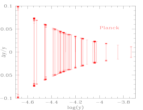
Figure 6: The Compton parameter, $y$, as Planck will measure for individual clusters. The brightest clusters will be measured to about $1\%$, and the dimmer clusters to about $10\%$.

The discussion above concludes that we cannot expect to measure the sub-dominant SZ parameters, however, what about the dominating Compton parameter, $y$. Fortunately this can be measured by Planck, and even to a very good precision.

The Compton parameter will be measured to about $1\%$ for the brightest clusters, and to about $10\%$ for the dimmer clusters (see fig. 6). This is very good news, because these numbers were obtained under the (rather pessimistic) assumption that we don’t know the spectral behaviour of all the non-removed contaminations. Thus, the accuracy with which Planck will measure $y$ may be even better.

We therefore conclude that Planck will measure a very large number of clusters, of the order 10 thousand, and the Compton parameter for each individual clusters will be measured to a few percent. This is what will give us a great catalogue for future targeted SZ experiments. All in all, Planck will measure the CMB accurately, and also provide a cluster catalogue which is larger, deeper and has more sky-coverage than any other existing catalogue. Naturally, one can use Planck for investigating less conventional (more funny?) physics, such as asteroids [57], highly relativistic electrons [58] etc, but I will leave that discussion for another good day.

7 Conclusions

The Planck satellite is a true piece of art, which will provide impressive information about the CMB sky. The SZ signal can easily be removed, and will not be a problem for CMB parameter extraction.

Planck will also give us a cluster catalogue which is larger, deeper and has more sky-coverage than any other existing catalogue. The Compton parameter for the individual clusters in this catalogue will be measured to $1\%$ accuracy for the brightest clusters, and to about $10\%$ for the dimmer clusters. Such a catalogue is very useful for future targeted SZ studies.

I have argued why I personally believe that the systematic errors for the individual clusters are still so hard to assess, that cosmological parameter extraction with this cluster sample will be very difficult. My view is rather conservative, so this leaves space for pleasant surprised when we will analyse the coming Planck data carefully.

- [1] \BYThe Planck collaboration http://astro.estec.esa.nl/Planck
- [2] \BYBalbi A. et al. \INApJ5882003L5
- [3] \BYMelchiorri A. arXiv:hep-ph/0311319.
- [4] \BYBowen R. et al. \INMNRAS3342002760
- [5] \BYMennella A. et al. \INAIP Conf. Proc.7032004401
- [6] \BYLamarre J. M. et al. \INNew Astronomy Reviews4720031017
- [7] \BYVilla F. et al. \INAIP conf. Proc.6162002224
- [8] \BYYurchenko V., Murphy J. A. and Lamarre J. M. arXiv:astro-ph/0205269
- [9] \BYChiang L. Y. and Naselsky P. arXiv:astro-ph/0303140
- [10] \BYAghanim N. et al \INA&A32519979
- [11] \BYWhite M. J. \INApJ5972003650
- [12] \BYGeisbuesch J., Kneissl R. and Hobson M. arXiv:astro-ph/0406190.
- [13] \BYRephaeli Y. arXiv:astro-ph/0110510.
- [14] \BYSadeh S. and Rephaeli Y. \INNew Astron.92004159
- [15] \BYHannestad S. et al \INAstropart. Phys.172002375
- [16] \BYBouchet F. R. and Gispert R. \INNew Astron.41999443
- [17] \BYHerranz D. et al \INMNRAS33620021057
- [18] \BYDiego J. M., Hansen S. H. and Silk J. \INMNRAS3382003796
- [19] \BYHerranz D. et al arXiv:astro-ph/0406226.
- [20] \BYForni O. and Aghanim N. arXiv:astro-ph/0402333.
- [21] \BYSunyaev R.A. and Zel’dovich Ya.B. \INComments Astrophys. Space Phys.41972173
- [22] \BYGull S. F. and Northover K. J. E \INNature2631976572
- [23] \BYLake G. and Partridge R. B. \INNature2701977502
- [24] \BYLaRoque S.J. et al arXiv:astro-ph/0204134
- [25] \BYDe Petris M. et al \INApJ5742002L119
- [26] \BYWright E. L. \INApJ2321979348
- [27] \BYDolgov A. D. et al. \INApJ554200174
- [28] \BYRephaeli Y. \INApJ445199533
- [29] \BYShimon M. and Rephaeli Y \INNew Astron.9200469
- [30] \BYItoh N. et al \INMNRAS3272001567
- [31] \BYItoh N. and Nozawa S. \INA&A4172004827
- [32] \BYPointecouteau E., Giard M., Barret D. \INA&A336199844
- [33] \BYHansen S. H., Pastor S. and Semikoz D. V. \INApJ5732002L69
- [34] \BYHansen S. H. \INNew Astronomy92004279
- [35] \BYHansen S. H. \INMNRAS3512004L5
- [36] \BYSchulz A. E. and White, M. J. \INApJ5862003723
- [37] \BYSchafer B. M. et al arXiv:astro-ph/0407089
- [38] \BYSchafer B. M. et al arXiv:astro-ph/0407090
- [39] \BYMoscardini L. et al. \INMNRAS3352002984
- [40] \BYKay S. T., Liddle A. R. and Thomas P. A. \INMNRAS3252001835
- [41] \BYNavarro J. F., Frenk C. S. and White S. D. M. \INApJ4621996563
- [42] \BYMoore B. et al \INApJ4991998L5
- [43] \BYHansen S. H. \INMNRAS3522004L41
- [44] \BYCarlstrom J. E., Holder G. P. and Reese E. D. \INAnn. Rev. Astron. Astrophys.402002643
- [45] \BYCavaliere and Fusco-Femiano \INA&A491976137
- [46] \BYHansen S. H. and Stadel J. \INApJ5952003L37
- [47] \BYHansen S. H. arXiv:astro-ph/0310302
- [48] \BYAghanim N. et al \INJCAP03052003007
- [49] \BYHaehnelt M. G. and Tegmark M. \INMNRAS2791996545
- [50] \BYVielva P. et al \INMNRAS344200389
- [51] \BYHerranz et al. D. Herranz, J. Gallegos, J. L. Sanz and E. Martinez-Gonzalez, \INMNRAS3342002533
- [52] \BYStolyarov V. et al. \INMNRAS336200297
- [53] \BYHolder G. P. \INApJ580200236
- [54] \BYWhite M. J. and Majumdar S. \INApJ6022004565
- [55] \BYKnox L, Holder G. P. and Church S. E. \INApJ612200496
- [56] \BYAghanim N., Hansen S. H. and Lagache G. arXiv:astro-ph/0402571
- [57] \BYCremonese G. et al. \INNew Astron.72002483
- [58] \BYEnsslin T. A. and Hansen S. H. arXiv:astro-ph/0401337