MAGNETICALLY-CONTROLED SPASMODIC ACCRETION DURING STAR FORMATION: II. RESULTS

Abstract

The problem of the late accretion phase of the evolution of an axisymmetric, isothermal magnetic disk surrounding a forming star has been formulated in a companion paper. The “central sink approximation” is used to circumvent the problem of describing the evolution inside the opaque central region for densities greater than $10^{11}$ $\rm{cm}^{-3}$ and radii smaller than a few AUs. Only the electrons are assumed to be attached to the magnetic field lines, and the effects of both negatively and positively charged grains are accounted for.

After a mass of $0.1$ $M_{\odot}$ accumulates in the central cell (forming star), a series of magnetically driven outflows and associated outward propagating shocks form in a quasi-periodic fashion. As a result, mass accretion onto the protostar occurs in magnetically controlled bursts. We refer to this process as spasmodic accretion. The shocks propagate outward with supermagnetosonic speeds. The period of dissipation and revival of the outflow decreases in time, as the mass accumulated in the central sink increases. We evaluate the contribution of ambipolar diffusion to the resolution of the magnetic flux problem of star formation during the accretion phase, and we find it to be very significant although not sufficient to resolve the entire problem yet. Ohmic dissipation is completely negligible in the disk during this phase of the evolution. The protostellar disk is found to be stable against interchange-like instabilities, despite the fact that the mass-to-flux ratio has temporary local maxima.

1 Introduction

In an accompanying paper (Tassis & Mouschovias 2004, hereafter Paper I) we formulated the problem of the formation and evolution of a nonrotating protostellar fragment in a manner that allows accurate modeling of the physics of the protostellar disk without the complication introduced by radiative transfer when the central protostar becomes opaque. In the present paper we follow the evolution until the mass of the central protostar grows to $1$ $M_{\odot}$. The importance and relevance of this problem as well as previous work on the subject were summarized in §1 of Paper I. The evolution of the system is described by the six-fluid MHD equations, in which neutral molecules, ions, electrons, neutral grains, positively and negatively charged grains are treated as distinct but interacting fluids. We use the “central sink” method to study the structure and evolution of the isothermal disk surrounding the forming protostar. The effects of the mass and magnetic flux accumulating in the central, opaque protostar on the isothermal disk are accounted for.

We include important physics ignored by previous calculations: (1) the decoupling of the ions from the magnetic field lines, which occurs at densities above $10^{8}\,{\rm cm^{-3}}$ (Desch & Mouschovias 2001) and which leaves the magnetic field frozen only in the much less massive and much more tenuous electron fluid; (2) the chemical and dynamical effects of the positively-charged grains, the abundance of which becomes significant in the same density regime. Phenomena that arise due to this new physics are discovered, such as the formation and dissipation of a series of shocks in a quasi-periodic fashion.

In §2 we summarize the most important results of the contraction phase prior to the introduction of the central sink. The evolution at later times, in the presence of a central sink, is described in §3. Specifically, we discuss: the evolution of the system until the first electron outflow occurs (§3.1); the establishment of a quasi-periodic magnetic cycle (§3.2) and the properties of one typical such cycle (§3.3) ; the time evolution of the mass, magnetic flux, and mass-to-flux ratio in the central protostar (§3.4); the properties of the shock in the neutral fluid (§3.5); and the evolution of the period of the magnetic cycle (§3.6). Finally, we investigate the stability of the supercritical core against a magnetic interchange instability (§3.7). The most important conclusions are summarized in §4.

2 Contraction Prior to the Central Sink Approximation

In order to obtain the proper initial conditions for the calculation of the collapsing cloud after the introduction of the central sink, we follow the ambipolar-diffusion–induced formation and contraction of a protostellar core in the absence of a central sink up to a central neutral density in excess of $10^{11}$ ${\rm cm^{-3}}$. The initial state is an exact equilibrium state in the absence of ambipolar diffusion, as in Ciolek & Mouschovias (1993). We reproduce the results presented by Desch and Mouschovias (2001), who studied the formation of protostars up to a central density $\gtrsim 10^{12}$ ${\rm cm^{-3}}$ using a modified ZEUS-2D code. This attests to the accuracy of the two very different numerical codes. We summarize the main features of the evolution, emphasizing those that are different from the corresponding results of Ciolek and Königl (1998), because of our more accurate physical assumptions (i.e., flux-freezing in the electrons instead of the ions, and inclusion of positive grains) and more appropriate numerical treatment of both the $r$-component of the magnetic field and the boundary conditions at the surface of the central sink, at $r=R{\rm inner}=7.31$ AU.

Starting from a reference state at temperature $T=10$ K, a uniform magnetic field $B_{\rm ref}=35.26$ ${\rm\mu G}$, and a central mass-to-flux ratio $\mu_{\rm c,0}=0.256$, in units of the critical value for collapse, we calculate the initial equilibrium state. The model cloud in equilibrium has a total mass $M=96.6$ $M_{\odot}$ and central number density $n_{\rm n,c0}=2700$ ${\rm cm^{-3}}$. It is thermally supercritical (the Bonnor-Ebert critical mass is only $M_{BE}=3.5//M_{\odot}$; see Bonnor 1956; Ebert 1955, 1957) but magnetically subcritical. At time $t=0$ we start the simulation by “turning on” ambipolar diffusion.

Figure 1: Evolution of central number density of neutrals normalized to its initial value $n_{\rm n,c0}=2.7\times 10^{3}$ ${\rm cm^{-3}}$ as a function of time (normalized to the initial central flux-loss timescale, $\tau_{\rm\Phi,c0}=1.88\times 10^{7}$ yr) before the introduction of the central sink. The “star” on the curve marks the instant at which the central mass-to-flux ratio becomes equal to its critical value for collapse.

Figure 1 shows the evolution of the central neutral density, $n_{\rm n,c}$, normalized to its initial equilibrium value $n_{\rm n,c0}$, as a function of time, normalized to the initial central flux-loss timescale, $\tau_{\Phi,c0}\equiv[\Phi_{B}/(d\Phi_{B}/dt)]_{c0}$. The two distinct phases in the evolution of the model cloud are evident. Initially, during the ambipolar-diffusion–controlled phase, the central density increases slowly, at the initial central flux-loss time, by a factor $\simeq 30$ in the first $1.598\times 10^{7}$ ${\rm yr}$. By then the central mass-to-flux ratio has exceeded the critical value for collapse and the evolution changes dramatically after this time. The now magnetically (and thermally) supercritical core contracts dynamically (but is not free-falling) and the central density increases (from $\approx 7\times 10^{4}$ ${\rm cm^{-3}}$) rapidly by seven orders of magnitude in the next $2\times 10^{5}$ ${\rm yr}$.

Figure 2: Central abundances (electrons e, ions i, negative grains ${\rm g_{-}}$, positive grains ${\rm g_{+}}$, and neutral grains ${\rm g_{0}}$) relative to the total density of neutrals versus the central neutral density $n_{\rm n,c}$, normalized as in Fig. 1.

The central relative abundances of all species, $\chi_{\rm s}\equiv n_{\rm s}/n_{n}$ (where $s={\rm i}$, e, ${\rm g_{+}}$, ${\rm g_{-}}$, ${\rm g_{0}}$) are shown in Figure 2 as functions of the neutral density. For low densities, corresponding to the cloud envelopes and the early stages of the evolution of the central region, the atomic and molecular ions are slightly more abundant than the electrons and much more abundant than any grain species. The grains are primarily negatively charged because of more efficient electron (than ion) attachment onto neutral grains. During the early, ambipolar-diffusion–controlled phase of the evolution, the fractional abundances of all grain species decrease, because they are attached to magnetic field lines and are “left behind” as the neutrals, under the action of their self-gravity, contract through all charged species. Thus the total central dust-to-gas mass ratio decreases initially. For densities higher than $10^{10}$ ${\rm cm^{-3}}$, the grains become the dominant charge carriers. Now the grains are primarily neutral and, for even higher densities, the positive grains are almost as abundant as the negative grains. Since the electrons are depleted (by attachment onto the neutral grains) faster than the ions, the ions become considerably more abundant than the electrons.

Figure 3: Ambipolar-diffusion-induced evolution of model cloud. Spatial profiles are shown at ten different times before the introduction of the central sink, namely at $t$ = 0, 13.66, 16.99, 17.43, 17.49, 17.5044, 17.5072, 17.5079, 17.50812, and 17.50816 Myr. The radial coordinate is normalized to $R_{0}=4.23$ pc. (a) Neutral density $n_{\rm n}$, normalized to its initial central equilibrium value $n_{\rm n,c0}$ $(=2.7\times 10^{3}$ ${\rm cm^{-3}}$); (b) $z$-component of the magnetic field $B_{z}$ normalized to the reference-state magnetic field, $B_{\rm ref}$ $(=35.27$ ${\rm\mu G}$); (c) $r$-component of the magnetic field $B_{r}$ normalized to the reference-state magnetic field, $B_{\rm ref}$; (d) radial velocity of the neutrals $v_{\rm n}$ normalized to the isothermal sound speed, $C$ $(=0.188$ km ${\rm s^{-1}})$; (e) radial drift velocity $v_{\rm D}$ between electrons and neutrals normalized to the sound speed in the neutrals, $C$; (f) mass-to-flux ratio $M/\Phi_{\rm B}$, normalized to the critical value for a thin disk $1/(2\pi G^{1/2})$.

Figures 3a - 3f show physical quantities as functions of the radial coordinate $r$ (normalized to the initial cloud radius $R_{0}=4.23$ ${\rm pc}$) at ten different times, $t_{j}$ $(j=0,1,...,9)$. These times $t_{j}$ are chosen such that the central density has increased by a factor $10^{j}$ $(j=0,1,...,9)$ relative to its initial equilibrium value. An asterisk on a curve marks the radius of the magnetically supercritical core at that time; i.e., the total mass-to-flux ratio within this radius is equal to the critical value.

Figure 3a exhibits the number density of the neutral particles (normalized to its initial central value) as a function of radius at ten different times (see caption for values). The density is almost uniform in the innermost part of the core, where the thermal-pressure forces dominate and smooth out all density fluctuations. At late times, the density follows a nearly power-law dependence on the radius outside the central region. The mean (logarithmic) slope in this region is 1.7. The envelope of the cloud where most of the mass resides hardly changes during the evolution, remaining magnetically supported. The mass of the supercritical core at the last time output, when $n_{n,c}/n_{n,c0}=10^{9}$, is $7.7$ $M_{\odot}$, and an amount of mass equal to $1$ $M_{\odot}$ is contained within the radius $r/R_{0}=5\times 10^{-3}$, i.e., inside $r=4.36\times 10^{3}$ AU.

Figure 4: The ion attachment parameter, $\Delta_{\rm i}$, as a function of $r/R_{0}$ at the same ten times as in Figure 3. $\Delta_{\rm i}=1$ means perfect attachment to, and $\Delta_{\rm i}=0$ complete detachment (of the ions) from the field lines.

The spatial structure of the $z$-component of the magnetic field is displayed in Figure 3b, at the same ten times as in Figure 3a. It is qualitatively similar to the density distribution, with a nearly uniform (but more extended) region near the origin and an almost power-law region in the rest of the collapsing core, characterized by a mean (logarithmic) slope of $0.7$. During the dynamical stage of contraction, $B_{\rm c}\propto n_{\rm c}^{0.47}$ (see review by Mouschovias 1987), so that each factor of 10 increase in $n_{\rm n,c}$ raises $B_{z,{\rm c}}$ by a factor of about 3. This behavior breaks down above a central density of about $10^{10}$ ${\rm cm^{-3}}$. Thereafter, the collapse of the matter in the innermost region of the supercritical core does not much alter the magnetic field structure because of re-awakening of ambipolar-diffusion.

The radial component of the magnetic field, $B_{r}/B_{\rm ref}$, just above $z=Z$, is shown as a function of radius in Figure 3c, at the same ten times as in Figure 3a . Comparison to Figure 3b reveals that $B_{r}<B_{z}$ at all times and at all radii.

Figure 3d similarly shows the radial infall velocity of the neutrals, $v_{{\rm n},r}$, (normalized to the isothermal sound speed) as a function of $r/R_{0}$. Once a magnetically supercritical core has formed, matter inside it contracts much more rapidly than matter in the envelope. The infall velocity remains subsonic everywhere throughout the run.

The drift velocity $v_{\rm D}\equiv v_{{\rm e},r}-v_{{\rm n},r}$ (normalized to the isothermal sound speed) is shown in Figure 3e as a function of $r/R_{0}$. Since electrons are attached to the magnetic field lines, their velocity represents that of the field lines as well. Prior to the formation of the supercritical core ($t<t_{2}$), ambipolar diffusion controls the infall of the neutrals throughout the cloud. At $r/R_{0}=0.15$ both the neutral infall speed (3d) and the drift speed are maximum, with $v_{\rm D}\backsimeq-v_{{\rm n},r}$. These two speeds are equal and opposite because the magnetic field lines are essentially “held in place” (i.e., $|v_{{\rm e},r}|\ll|v_{{\rm n},r}|$) as the neutrals contract through them. Ambipolar diffusion continues to control the infall of the neutrals in the envelope at all times, while the smaller drift speed inside the supercritical core at times $t_{7}\geq t\geq t_{2}$ indicates the dragging of the field lines inward with the neutrals. The increase of the drift velocity at the innermost part of the supercritical core for densities above $10^{10}$ ${\rm cm^{-3}}$ ($t>t_{7}$) reveals that the neutrals are contracting significantly faster than the field lines (rejuvenation of ambipolar diffusion) leading to the lack of increase of $B$ with increasing $n_{\rm n}$, as shown in Figure 3b.

Figure 3f shows the mass-to-flux ratio $M/\Phi_{\rm B}$, normalized to the critical value, $1/(2\pi G^{1/2})$, as a function of $r/R_{0}$, at the same times as in Figure 3a. Initially the cloud has a subcritical value at the center. The mass-to-flux ratio increases during the ambipolar-diffusion–controlled phase of the evolution. A supercritical core (marked by an asterisk) forms after the second curve. During the dynamical phase of contraction the mass-to-flux ratio approaches an asymptotic value 2 - 3, but after the density at the center exceeds $10^{10}$ ${\rm cm^{-3}}$ the mass-to-flux ratio increases again, indicating the re-awakening of ambipolar diffusion, as found by Desch & Mouschovias (2001).

Finally, the ion attachment parameter

$$\Delta_{\rm i}\equiv\frac{v_{\rm i}-v_{\rm n}}{v_{\rm e}-v_{\rm n}}$$ (1)

is shown as a function of $r/R_{0}$ in Figure 4, at the same times as in Figure 3a. This parameter is a measure of how well the ions are coupled to the magnetic field. If $\Delta_{\rm i}=1$, the ions move with the electrons and the magnetic field, while if $\Delta=0$, the ions are completely detached from the magnetic field and fall in with the neutrals. Inside the region of radius $r\approx 2\times 10^{-5}R_{0}=17.5$ AU, the ions begin to detach from the field lines at densities as low as $10^{8}$ ${\rm cm^{-3}}$ (curve labeled $t_{5}$) and are almost completely detached by a density $10^{10}$ ${\rm cm^{-3}}$. This causes the re-awakening of ambipolar diffusion, witnessed in Figures 3b, 3c, 3e and 3f. The assumption of flux-freezing in the ion fluid (used by Ciolek & Konigl 1998) is therefore invalid for densities greater than $10^{8}$ ${\rm cm^{-3}}$.

3 The CSA Calculation

Now we introduce the central sink at radius $R_{\rm inner}=7.31$ ${\rm AU}$. The density at this position is $6.5\times 10^{10}$ ${\rm cm^{-3}}$ and the mass initially contained in the central sink is $M=8\times 10^{-4}$ ${\rm M_{\odot}}$, which is negligible compared to the mass of the cloud or the supercritical core ($M_{\rm core}=7.6$ ${\rm M_{\odot}}$). We let the previous calculation go to higher central densities ($\approx 10^{12}$ ${\rm cm^{-3}}$) in order for the density profile of Figure 3a to establish an almost power-low shape at all densities of interest, and the central thermal lengthscale to become much smaller than the radius of the central sink. For this part of the calculation we use a stationary grid with 160 zones.

3.1 Evolution to Resurrection of Ambipolar Diffusion and
First Electron Outflow

Figure 5 shows various quantities as functions of $r/R_{0}$, at eight different times ($\Delta t$ = 0, 125, 316, 677, 1472, 3213, 6983 and 15170 yr). $\Delta t$ is the time elapsed since the beginning of the CSA calculation. Each successive time marks the doubling of the mass accumulated in the central sink. By the last time output shown in Figure 5a (curve 7), this mass is $0.1$ ${\rm M_{\odot}}$. An asterisk on a curve locates, as in Figures 3a-f, the instantaneous radius of the critical flux tube. The radius of the supercritical core does not change from its initial value during the evolution.

Figure 5: Spatial profiles of physical quantities at eight different times ($\Delta t$ = 0, 125, 316, 677, 1472, 3213, 6983 and 15169 yr), after the central sink is introduced. The radial coordinate is normalized to $R_{0}=4.23pc$ and the inner boundary (dashed line) is at $7.31$ AU. (a) Total mass in $M_{\odot}$; (b) Number density of neutrals normalized to its central value in the reference state, $n_{\rm n,c0}=2.7\times 10^{3}$ ${\rm cm^{-3}}$; (c) $B_{z}$ normalized to its value in the reference state, $B_{\rm ref}=\,\,35.26{\rm\mu G}$; (d) $B_{r}$ normalized to $B_{\rm ref}$; (e) Radial velocity of neutrals, normalized to the isothermal sound speed, $C$; (f) Electron velocity, normalized to $C$; (g) Drift velocity of electrons with respect to the neutrals, normalized to $C$; (h) Mass accretion rate in ${\rm M_{\odot}/Myr}$; (i) Ratio of magnetic and gravitational force.

As the evolution progresses, the neutral number density departs from the established power-law of the pre-CSA evolution, and this deviation propagates to larger and larger radii (Fig. 5b). A similar behavior is exhibited by the $z-$ and $r-$ components of the magnetic field (Figs. 5c and 5d respectively). In the region $5\times 10^{-4}\lesssim r\lesssim 10^{-3}R_{0}$, $B_{r}$ becomes greater than $B_{z}$, implying that magnetic-tension forces become more important than magnetic-pressure forces in this region. However, in the cells adjacent to the sink, $B_{z}$ is always larger than $B_{r}$.

An important feature of the evolution of $B_{z}$ is the presence of a narrow radial region in which the field rises steeply by almost an order of magnitude. The radial position of this magnetic wall coincides with the position of a peak in the ratio of magnetic and gravitational forces acting on the neutral fluid (Fig. 5i). The strong magnetic force decelerates the neutrals (Fig. 5e) and eventually causes a slight outflow (positive velocity) in the electron fluid in the region $r\lesssim 7\times 10^{-5}R_{0}$ (last curve in Fig. 5f). As we’ll see below, this magnetic wall forms, dissipates and reappears repeatedly during the evolution of the model cloud.

The reason for the formation of the magnetic wall is revealed by the time-evolution of the electron velocity profiles (Fig. 5f). Close to the sink, the resurrection of ambipolar diffusion is manifested as a deceleration of the electron fluid without a corresponding decrease of the velocity of the neutral fluid. By $\Delta t=3213{\rm\,yr}$ (curve labeled by 5), the electron infall speed at the cell adjacent to the sink has decreased to zero, while at larger radii the electrons are still falling in. This causes a magnetic flux pileup, and further deceleration of the electrons at greater and greater radii. Eventually, the magnetic force becomes large enough to drive a slight outflow of the electrons in the region $r\lesssim 7\times 10^{-5}R_{0}=61$ AU at time $\Delta t=15,184$ yr (see last curve in Fig. 5f).

The response of the neutral fluid to the changes in the magnetic force is shown in Figure 5e, which exhibits the velocity of the neutrals versus radius at the same times as in Figure 5a. By the time $\Delta t=677$ yr (curve labeled by 3 in Fig. 5e) the maximum infall speed has become supersonic (and supermagnetosonic), and a shock has formed in the neutral fluid, which propagates outward at subsequent times. At radii smaller than the location of the shock front (i.e., behind the shock) the neutrals decelerate, and reach a minimum infalling speed at a radius slightly smaller than the location of the maximum of the ratio $F_{M}/F_{G}$. At yet smaller radii, the neutrals are reaccelerated by the gravitational field of the mass already in the central sink.

The resurrection of ambipolar diffusion is illustrated clearly in Figure 5g, which shows the drift velocity of the electrons relative to the neutrals. Within the supercritical core, the drift velocity develops a plateau at a low value, corresponding to the ineffectiveness of ambipolar diffusion during a large part of the dynamical phase of contraction. However, a peak develops in the drift velocity at small radii at later times. This implies resurrection of ambipolar diffusion because the ambipolar-diffusion timescale $\tau_{AD}\sim r/v_{D}$ decreases locally. Inward of the peak of $v_{D}$ there is a local minimum, corresponding to the local deceleration of the neutrals close to the position of the magnetic force maximum. Closer to the boundary of the central sink, the drift speed rises sharply and monotonically, because the electrons are held back by the magnetic force while the neutrals get reaccelerated by the mass already accumulated in the central sink.

Figure 6: Spatial profiles, after the central sink approximation, of the attachment parameter of the ions shown at the same times as in Fig. 5.

The mass infall rate (Fig. 5h) is almost a mirror image of the velocity of the neutral fluid. Initially it increases as $r$ decreases, but, after the formation of the shock in the neutrals, it exhibits a steep drop at the position of the shock. This feature eventually develops into a clear minimum, corresponding to the minimum infall velocity of the neutral fluid.

Finally, the ion attachment parameter is shown in Figure 6 as a function of $r/R_{0}$, at the same eight times as in Figure 5a. As time progresses, the region of almost complete detachment (small values of $\Delta_{\rm i}$) of the ions from the field lines expands outward. This is a consequence of the significant increase of the density at greater and greater radii (Fig. 5b), deviating from the power-law profile established in the pre-CSA calculation, without a corresponding increase of $B_{z}$. An increase of the density leads to more frequent collisions of ions with neutral particles causing them to detach from the field lines, while an increase of the magnetic field leads to better attachment of the ions. By the time $\Delta t=15,170{\rm\,yr}$, at a radius of $r\approx 5\times 10^{-5}R_{0}$ the density has increased by almost two orders of magnitude, while $B_{z}$ has increased by only one order of magnitude. At the same time, at an inner radius of $r\approx 10^{-5}R_{0}$ the density has increased by a factor of three and $B_{z}$ has increased by more than an order of magnitude. Consequently at small radii, near the central-sink boundary, the ions become somewhat better coupled to the field lines than they were at the beginning of the run; $\Delta_{i}$ increases from $0.02$ to almost $0.1$.

3.2 Quasi-Periodic Magnetic Cycle

Figure 7: Profiles of the neutral velocity (upper panel) and the electron velocity (lower panel) normalized to the isothermal sound speed in the neutrals ($C=0.188$ km ${\rm s^{-1}}$). The leftmost, middle, and rightmost frames correspond to the first, second and third magnetic cycles, respectively. Each curve in these plots corresponds to a specific instant in each magnetic cycle, with the curve numbers (1-3) increasing from earlier to later times.

After the first electron (slow) outflow, the system enters a phase where the magnetic flux transport, as well as the response of the other quantities to the evolution of the magnetic flux, exhibit a quasi-periodic behavior.

To demonstrate this behavior, we have plotted in Figure 7 profiles of the velocities of the neutrals (upper panel) and the electrons (lower panel) for three instances of each of the first three “magnetic cycles” after the first electron (slow) outflow. The leftmost frames correspond to the first cycle, the middle frames correspond to the second cycle, and the rightmost frames to the third cycle. We focus our attention to the region $r\lesssim 2\times 10^{-4}R_{0}=174$ AU. The first (earliest) curve for each cycle corresponds to infalling velocities at all radii for both neutrals and electrons. Flux is being accumulated at small radii during this phase of the cycle, since $|v_{\rm n}|\gg|v_{\rm e}|$. At the instant corresponding to the second curve of each cycle, the enhanced magnetic force due to the accumulated flux has reduced the electron velocity to essentially zero and has significantly decelerated the neutrals in the first two cycles while it has produced a mild outflow in the third cycle. Finally, the third curve of each cycle corresponds always to outflow in the electron fluid, and very small infalling velocities (in the first cycle) or outflows (in the next two cycles) in the neutrals. The outflow spreads the accumulated flux to larger radii. As a result, gravity dominates again, and the neutrals get reaccelerated inward, dragging with them the electrons. The inflow of electrons recreates the magnetic wall, and the cycle repeats itself.

Other than the repetitive pattern of this behavior, it is also important to note that the amplitude of the variation in the velocities of the neutrals and electrons increases with each cycle. We will discuss in detail the evolution of the amplitude and the period of the magnetic cycle after we analyze the behavior of other physical quantities during a typical cycle.

3.3 Analysis of a Typical Magnetic Cycle: The Rise and Fall of a Magnetic Wall

Figures 8 and 9 show the evolution of the radial profiles of the neutral number density, magnetic field, radial velocity of the neutrals and electrons, the ratio of magnetic and gravitational forces, and the attachment parameters of the ions, the negative and positive grains during a typical quasi-periodic cycle introduced above. For clarity, the duration of a single cycle has been broken into two parts. During the first part, shown in Figure 8, at radii smaller than the location of the maximum outflow velocity of the electrons there is essentially no infall of magnetic flux, i.e., the velocity of the electrons is either positive or almost zero. During the second part of the cycle, shown in Figure 9, the electrons are reaccelerated inward by the infalling neutrals (they acquire negative velocities) at radii smaller than the position of the fastest outflow. The dashed curve in Figure 9 corresponds to the first snapshot of the next cycle, showing the re-establishment of outflow velocities close to the central sink.

The number density of the neutral particles, as seen in Figure 8a, decreases with time in the region where it has deviated from its established global profile. This is so because some matter moves outward, as seen in Figure 8d (region of positive $v_{n}$), while other matter falls into the central sink - in the cells adjacent to the sink the neutrals still have negative velocities. As time progresses, the number density of the neutrals develops a local maximum at moderate radii, at the position of the shock, where both the neutral outflow behind the shock as well as the neutral infall ahead of the shock are responsible for a pileup of matter. As the shock propagates outward, this local maximum follows the shock, staying right behind it.

Figure 8: Spatial dependence of physical quantities during the first half-period of a magnetic cycle. Normalizations are as in Fig. 5. (a) Number density of neutrals; (b) $z-$component of the magnetic field $B_{z}$; (c) $r-$component of the magnetic field $B_{r}$; (d) Radial velocity of neutrals $v_{\rm n}$; (e) Radial electron velocity $v_{\rm e}$; (f) Ratio of magnetic and gravitational forces $F_{\rm M}/F_{\rm G}$; (g) Attachment parameter of ions $\Delta_{\rm i}$; (h) Attachment parameter of negatively charged grains $\Delta_{\rm g-}$; (i) Attachment parameter of positively charged grains $\Delta_{\rm g+}$

The $z$-component of the magnetic field (Fig. 8b) exhibits the sharp increase characteristic of the magnetic wall that drives the outflow. The position of this wall propagates outward in time, while the field strength at small radii decreases as the electron outflow redistributes the magnetic flux outward and arrests the accumulation of flux in this region. The $r-$component of the magnetic field (Fig. 8c), which is a measure of the deformation of the field lines, also decreases in time at small radii because of the local outflow of the electrons. This tendency of the electron outflow to straighten out the field lines at small radii is also responsible for the development of a local maximum in the spatial profile of $B_{r}$ at the position of the shock.

The most prominent features of the velocity profiles of the neutrals and the electrons (Figs. 8d and 8e, respectively) are of course the presence of the shock and the outflows. The positions of the maximum outflow velocity and that of the shock move outward, while the magnitude of the outflow velocity eventually decreases as the outflow in the electrons lowers the magnetic wall that drives it. This physical picture is also supported by Figure 8f, which shows the ratio of magnetic and gravitational forces. The peak of this ratio, identifying the position of the magnetic wall, does indeed move outward while at the same time decreasing in magnitude.

The attachment parameters of the ions and charged grains in the region $r\lesssim 2\times 10^{-4}R_{0}=175$ AU increase in time, in response to the significant decrease in density (which is accompanied by only a moderate decrease of the magnetic field). The effect is most pronounced for the ions and least pronounced for the positively charged grains.

The direction of change of the quantities in the innermost radii is reversed during the second part of the cycle, shown in Figure 9. The electron outflow in the first part of the cycle creates a deficit of magnetic flux behind the position of the maximum velocity outflow. This deficit can be seen in both the profiles of $B_{z}$ (Fig. 9b), where a local minimum develops immediately behind the location of the magnetic wall, and in the magnetic-to-gravitational force ratio (Fig. 9f) where a dip at values smaller than $1$ occurs behind (at smaller radii than) the maximum.

As a result, in the region of this magnetic deficit, the gravitational force dominates and re-accelerates the neutrals inward. Figure 9d shows the progressively greater infalling velocities acquired by the neutrals in the region behind the outflow. In turn, the infalling neutrals drag with them the electrons, and magnetic flux once again starts being transported inward behind the shock. The magnetic wall will now disperse much faster than at earlier times because accumulated flux is transported both outward (due to the electron outflow that continues) and inward (due to the re-accelerated infall of the electrons). However, as the electrons acquire greater infall velocities, a new accumulation of flux will occur near the original position of the magnetic wall, and a new magnetic wall will form there. Eventually, this magnetic wall drives a new outflow, and a new magnetic cycle begins. The beginning of the new cycle is marked by the dashed curve in the plots of Figure 9. Note that the electrons respond much faster than the neutrals to the accumulation of magnetic flux. The neutrals have to overcome their relatively large inertia, that tends to keep them falling inward, before they can join the electron outflow.

Figure 9: Spatial profiles of the same quantities as in Fig. 8, but during the second half-period of a magnetic cycle.

The rest of the quantities in the second part of the cycle change in response to the negative velocities acquired by the neutrals and the electrons. The neutral number density at the inner radii increases in time (Fig. 9a) as new material starts flowing inward. In the same way, $B_{z}$ and $B_{r}$ (Figs. 9b and 9c, respectively) increase at small radii in response to the inward transport of magnetic flux by the electrons. Finally, the attachment parameters of ions and charged grains decrease with time close to the central sink (Figs. 9g, 9h and 9i, respectively), in response to the increasing number density of neutrals in the same region, which leads to more frequent collisions and detachment of the charged species from the field lines.

Figure 10: (a) Time evolution of mass of the central sink (in ${\rm M_{\odot}}$) (b), Mass-to-flux ratio of central sink normalized to the critical value for collapse, $1/(2\pi G^{1/2})$. (c) Rate of mass accretion in the central sink (in ${\rm M_{\odot}/Myr}$).

3.4 Time Evolution of Physical Quantities in the Forming Star

Figure 10 describes the evolution of the mass and magnetic flux accumulated in the central sink (the forming star). The total mass (in ${\rm M_{\odot}}$) is shown in Figure 10a. In our model, the time required for the sink mass to become equal to $1{\rm\,M_{\odot}}$ is $2.55\times 10^{5}{\rm\,\,yr}$. For comparison, Ciolek & Königl (1998) find that in their model the corresponding time interval is only $1.53\times 10^{5}{\rm\,\,yr}$. The multiple shocks formed during the magnetic cycles in our case, cause the mass accretion process to be both slower and spasmodic.

The effect of the magnetic cycle on the mass accretion rate (in ${\rm M_{\odot}/Myr}$) is demonstrated directly in Figure 10c. It initially increases because of the ever-increasing gravitational field strength due to accumulation of mass in the central sink. However, after the formation of the first shock (at $\approx 200{\rm\,\,yr}$), the mass accretion rate decreases again, in agreement with the findings of Ciolek & Königl (1998). At still later times, nevertheless, when the magnetic cycle becomes fully developed, the mass accretion rate starts to exhibit oscillations of large amplitude (of about one order of magnitude above and below the mean). This can be understood in terms of the evolution of the density in the innermost parts of the disk during one magnetic cycle. As an outflow in the neutrals is established from a certain radius outward, no new material accretes inward to replenish the matter lost to the sink, and the mass accretion rate decreases dramatically. Only after the magnetic wall is dispersed and the outflow in the neutrals is suppressed does the density of the innermost part of the disk increase again, and with it the mass accretion rate by the central sink. Thus, mass accretion onto the forming star occurs in magnetically controlled bursts. We refer to this process as spasmodic accretion.

The mass-to-flux ratio in the sink, normalized to the critical value for collapse ($1/2\pi\sqrt{G}$), also increases monotonically up to the point where the magnetic cycle is established (Fig. 10b). From that point on, the mass-to-flux ratio exhibits strong oscillations. Overall the mass-to-flux ratio increases by two orders of magnitude above the critical value. This flux loss, which is entirely due to ambipolar diffusion before the complete decoupling of the magnetic field from the matter, is an important contribution toward the resolution of the magnetic flux problem of star formation, although not yet sufficient to resolve the entire problem.

3.5 Properties of the Shocks in the Neutrals

Figure 11: (a) Velocity of the neutral fluid, normalized to the local magnetosonic speed $V_{\rm ms}$, as a function of $r/R_{0}$ at regular intervals of 250 yr, between $\Delta t=6\times 10^{4}$ and $\Delta t=2\times 10^{5}$ yr (b) Velocity of the shock normalized to $V_{\rm ms}$ as a function of time. (c) Mach number of shock with respect to the local magnetosonic speed as a function of time.

Figure 11 shows some properties of the shocks established in the neutrals during each magnetic cycle. Figure 11a exhibits the radial profile of the velocity of the neutral fluid normalized to the magnetosonic speed in intervals of 250 yr for the duration of the run. The average positions of the maximum infall velocity and the maximum outflow velocity are near each other and remain fixed in time during successive magnetic cycles. The magnetic cycle affects the entire supercritical core. It is also interesting to note that although the absolute value of the maximum infall velocity of the neutrals increases in time (as the mass of the sink and with it the gravitational field increase), the value of the maximum outflow velocity remains constant with respect to the magnetosonic speed, and almost twice as large.

Figure 11b shows the speed of outward propagation of the shock normalized to the magnetosonic speed, for a series of magnetic cycles taking place between $6\times 10^{4}$ and $2\times 10^{5}$ yr after the introduction of the central sink. The speed of the shock varies between 5 and 1 times the magnetosonic speed, and generally tends to decrease as the shock propagates outward. At almost all times the shock speed is supermagnetosonic. This is in contrast to the results of Ciolek & Königl (1998), who found that the shock propagation is subsonic.

Figure 11c shows the Mach number $\mathcal{M}$ with respect to the local magnetosonic speed for the same time interval as in Figure 11b. In each cycle, the shock Mach number varies between about 6 and 2, with a trend to decrease as the shock propagates outwards.

3.6 Evolution of the Period of the Magnetic Cycle

Figure 12: Evolution in time of the period of the magnetic cycle in years (data points). The error bars are due to the finite time resolution with which output is obtained from the simulation. The solid curve is the average ambipolar-diffusion (magnetic flux-loss) timescale at the position of the maximum infall/outflow velocity of the neutrals.

The data points in Figure 12 show the period of the magnetic cycle in years. The “error bars” are due to the finite time resolution with which the output used to determine the duration of each cycle is obtained from the simulation. The solid curve is the average ambipolar-diffusion (magnetic flux-loss) timescale, $\tau_{\Phi}=r/2v_{D}$ (Mouschovias 1991, eq. [31]) at the position of the maximum infall/outflow velocity of the neutrals. This was calculated by averaging the drift velocity of the electrons over each cycle at the position where the maximum neutral infall/outflow occurs. This position is, as we already discussed, the same for all cycles. This average drift velocity was then used to obtain the average magnetic flux-loss timescale. The agreement between the flux-loss timescale and the duration of each cycle is excellent. This is due to the fact that the average flux-loss timescale represents the time required to rebuild the magnetic wall after it is dispersed by the outflow of the electrons. The rebuilding of the magnetic wall is the slowest phase (bottleneck) of the cycle, and for this reason determines the entire duration of each cycle. The decrease of the duration of the magnetic cycle with time is due to the decrease of the associated ambipolar-diffusion timescale (which decreases as the gravitational field increases, and the maximum infall velocity of the neutrals increases as well).

3.7 Stability of the Supercritical Core Against Magnetic Interchange

Figure 13 (top row) exhibits the local mass-to-flux ratio, $dM/d\Phi_{B}=\sigma_{n}/B_{z}$ (normalized to the critical value for collapse) as a function of position at $t=33500,36000,37251$ yr (from left to right) after the introduction of the central sink (curves 1 of Fig. 8; and curves 6, 8 of Fig. 9, respectively). At radii smaller than the position of the shock ($\sim 10^{-3}R_{0}$), the local mass-to-flux ratio increases with increasing radius. This is a necessary (although not sufficient) condition for the development of the magnetic interchange instability (Spruit & Taam 1990; Lubow & Spruit 1995). That the region behind a hydromagnetic shock in a collapsing disk is prone to the interchange instability was speculated by Li & McKee (1996) and also found in the simulation of Ciolek & Königl (1998). It is therefore of interest to examine the stability of the supercritical core with respect to this instability.

Two effects can prevent the magnetic interchange instability from developing: damping due to inefficient coupling between the magnetic field and the neutral fluid, and erasing of the perturbations due to the fast inflow of the neutrals (Ciolek & Königl 1998). Therefore, the instability will be able to grow only if: (i) its growthtime is longer that the timescale of collisional coupling between the magnetic field and the neutral fluid (due to electron-neutral and/or ion-neutral collisions), $\tau_{\rm coll}$, and (ii) if its growthtime is smaller than the gravitational contraction timescale, $\tau_{\rm gr}\approx(r/|g|)^{1/2}$. This is the timescale that characterizes the (dynamic) flow in this region of the supercritical core.

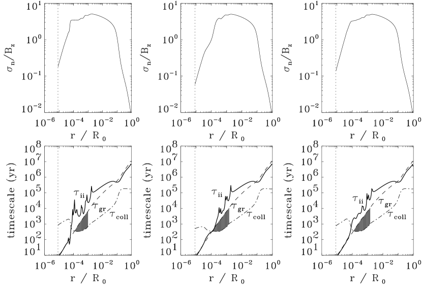
Figure 13: Upper panel: Local mass-to-flux ratio normalized to the critical value for collapse at $t=33,500$ yr (left); $t=36,000$ yr (middle); $t=37,251$ yr (right). Lower panel: Gravitational contraction timescale ($\tau_{\rm gr}$, dashed line), magnetic field - neutral fluid collisional coupling timescale ($\tau_{\rm coll}$, dot-dashed line), and growthtime of most unstable mode of interchange instability in hydrostatic equilibrium ($\tau_{\rm ii}$, bold solid line), as functions of $r$, at the same times as in the upper panel. The shaded area correspond to span of allowed instability growthtimes.

In the lower panel of Figure 13 we have plotted the gravitational-contraction (dashed line) and the collisional-coupling (dot-dashed line) timescales as functions of radius (normalized to $R_{0}$, as usual) at the same times as in the upper panel. Note that in our case, the timescale of collisional coupling between the magnetic field and the neutral fluid is given by

$$\frac{1}{\tau_{\rm coll}}=\frac{1}{\tau_{ne}}+\frac{\Delta_{i}}{\tau_{ni}},$$ (2)

properly accounting for the partial attachment (or full attachment, at certain regions in space) of the ions to the magnetic field (e.g., see Ciolek & Mouschovias 1993). This is in contrast to Ciolek & Königl (1998) who used $\tau_{\rm coll}=\tau_{ni}$ (a much smaller value than that given by eq. [2]) for their corresponding stability check, since in their model the ions were assumed to be always attached to the magnetic field.

The shaded region in each graph in the lower panel of Figure 13 corresponds to the span of allowed instability growthtimes, i.e., growthtimes which are not excluded from developing due to negative slope in the local mass-to-flux ratio, or due to inefficient coupling between magnetic field and neutrals, or due to erasing of perturbations by the neutral flow.

The bold solid line is the growthrate for the most unstable linear interchange mode calculated for discs in hydrostatic equilibrium (Spruit & Taam 1990; Lubow & Spruit 1995),

$$\tau_{\rm ii}=\left(\frac{B_{z,{\rm eq}}B_{r,Z}}{2\pi\sigma_{\rm n}}\frac{d}{dr}\ln\frac{\sigma_{\rm n}}{B_{z,{\rm eq}}}\right)\,.$$ (3)

Since our system is not in equilibrium, and there is no exact force balance between magnetic and gravitational forces, the actual instability growthtime will be longer; thus the bold line represents a lower limit for the instability timescale.

The innermost region ($\lesssim 10^{-4}\approx 90$ AU), where the slope of the local mass-to-flux ratio is steepest and the growth of the instability is fast (small growthtime), is entirely excluded at all times due to inefficient coupling, since in this region the ions are detached from the magnetic field and the electrons are not as effective in coupling the neutrals to the field lines. At radii greater than the point of intersection of the two curves $\tau_{\rm coll}$ and $\tau_{\rm gr}$, the lower limit of the instability timescale, $\tau_{\rm ii}$, is always greater than the contraction timescale, so perturbations are swept away before they have an opportunity to grow. Therefore, the magnetic interchange instability is not at all relevant.

4 Conclusions

We have studied the structure of the magnetic accretion disk surrounding a forming star, using the central-sink approximation to make the problem tractable numerically. The differences in the formulation of the problem compared to previous work (Ciolek & Königl 1998) have been discussed in detail in Paper I.

Multiple shocks develop and propagate in the neutral fluid, associated with a quasi-periodic magnetic cycle. Flux accumulation close to the central sink leads to the formation of a region of enhanced magnetic field strength, a “magnetic wall”, where magnetic forces exceed the gravitational forces. The magnetic wall drives outflows in the neutrals and associated shocks. In time, the magnetic wall disperses, and the neutrals are reaccelerated inward behind the shock (at smaller radii), dragging with them the electrons and, consequently, magnetic flux (since the field is frozen in the electrons). Flux can then reaccumulate, and the magnetic wall gets recreated, which causes the magnetic cycle to repeat.

The shocks in the neutrals propagate outward with supermagnetosonic speeds in the rest frame of the central sink. This is in contrast to the slow accretion shock expected by Li & McKee (1996) and found numerically by Ciolek & Königl (1998) because they assumed that the magnetic flux is frozen in the ion fluid. The infall velocities of the neutrals in the rest frame of the shock vary between 2 and 6 times the magnetosonic speed.

The development and propagation of multiple outflows and shocks result in mass accretion onto the forming star that occurs in magnetically controlled bursts. We refer to this phenomenon as spasmodic accretion. During the outflow of the neutrals, the inner part of the disk is almost “emptied” of matter (its column density decreases significantly) and the mass accretion rate drops almost by two orders of magnitude below its maximum value. It is only when the neutrals get reaccelerated inward by the mass of the forming star that the inner part of the disk is refilled with matter and the mass accretion rate increases again. The time required for 1 ${\rm M_{\odot}}$ to accumulate in the central sink is $2.55\times 10^{5}\,{\rm yr}$, characteristic of the relatively inefficient accretion process due to the magnetically-driven, repeated outflows in the neutrals.

The radial extent of the region which is affected by the magnetic cycle (in which the velocity of the neutrals exhibits the quasi-periodic oscillation characteristic of the magnetic cycle) includes almost the entire magnetically supercritical core. The magnetically supported envelope, as expected, is not affected by the magnetic flux redistribution in the core.

The period of the magnetic cycle decreases in time, and is well represented by the local flux-loss (ambipolar-diffusion) timescale. This is expected because the bottleneck in the chain of events comprising the magnetic cycle is the rebuilding of the magnetic wall behind the outward propagating shock in the neutrals. This reaccumulation of flux does indeed occur on the ambipolar-diffusion timescale, and it becomes faster as time progresses, since the gravitational field (dominated by the central point mass) monotonically increases with time, thereby increasing the maximum infall velocity of the neutrals (which in turn drag the electrons inward).

We found that the magnetically supercritical core is stable against interchange-type instabilities. This result is in contrast to the predictions by Li & McKee (1996) and Ciolek & Königl (1998). The reason for this difference with the results of Ciolek & Königl is the fact that they assumed flux-freezing in the ions, which is not valid above $\sim 10^{8}$ ${\rm cm^{-3}}$ and which leads to much better coupling between the neutrals and the magnetic field in their calculation.

Ambipolar diffusion by itself during the accretion phase significantly contributes to the resolution of the magnetic flux problem of star formation by increasing the mass-to-flux ratio of the protostar by more than two orders of magnitude above its critical value. However, this is not sufficient to resolve the entire magnetic flux problem yet.

References

- Bonnor (1956) Bonnor, W. B. 1956, MNRAS, 116, 351
- Ciolek & Königl (1998) Ciolek, G. E. & Königl, A. 1998, ApJ, 504, 257
- Ciolek & Mouschovias (1993) Ciolek, G. E. & Mouschovias, T. Ch. 1993, ApJ, 418, 774
- Desch & Mouschovias (2001) Desch, S. J. & Mouschovias, T. Ch. 2001, ApJ, 550, 314
- Ebert (1955) Ebert, R. 1955, Zs. Ap., 37, 217
- Ebert (1957) Ebert, R. 1957, Zs. Ap., 42, 263
- (7) Li, Z.Y & McKee C.F. 1996, ApJ, 464, 373
- (8) Lubow, S. H. & Spruit, H. C. 1995, ApJ, 445, 337
- (9) Mouschovias, T. Ch. 1987, in Physical Processes in Interstellar Clouds, ed. G. E. Morfill & M. Scholer (Dordrecht: Reidel), 453
- (10) Mouschovias, T. Ch. & Morton, S. A. 1991, ApJ, 371, 296
- (11) Spruit, H.C. & Taam, R.E. 1990. A&A, 229, 475
- (12) Tassis & Mouschovias 2004a, ApJ submitted (Paper I)