New $VR$ magnification ratios of QSO 0957+561

Abstract

We present $VR$ magnification ratios of QSO 0957+561, which are inferred from the GLITP light curves of Q0957+561A and new frames taken with the 2.56m Nordic Optical Telescope about 14 months after the GLITP monitoring. To extract the fluxes of the two close components, two different photometric techniques are used: pho2comC and psfphot. From the two photometric approaches and a reasonable range for the time delay in the system (415–430 days), we do not obtain achromatic optical continuum ratios, but ratios depending on the wavelength. Our final global measurements $\Delta m_{AB}(\lambda_{V})$ = 0.077 $\pm$ 0.023 mag and $\Delta m_{AB}(\lambda_{R})$ = 0.022 $\pm$ 0.013 mag (1$\sigma$ intervals) are in agreement with the Oslo group results (using the same telescope in the same seasons, but another photometric task and only one time delay of about 416 days). These new measurements are consistent with differential extinction in the lens galaxy, the Lyman limit system, the damped Ly $\alpha$ system, or the host galaxy of the QSO. The possible values for the differential extinction and the ratio of total to selective extinction in the $V$ band are reasonable. Moreover, crude probability arguments suggest that the ray paths of the two components cross a similar dusty environment, including a network of compact dust clouds and compact dust voids. As an alternative (in fact, the usual interpretation of the old ratios), we also try to explain the new ratios as caused by gravitational microlensing in the deflector. From magnification maps for each of the gravitationally lensed images, using different fractions of the surface mass density represented by the microlenses, as well as different sizes and profiles of the $V$–band and $R$–band sources, several synthetic distributions of [$\Delta m_{AB}(\lambda_{V})$,$\Delta m_{AB}(\lambda_{R})$] pairs are derived. In some gravitational scenarios, there is an apparent disagreement between the observed pair of ratios and the simulated distributions. However, several microlensing pictures work well. To decide between either extinction, or microlensing, or a mixed scenario (extinction + microlensing), new observational and interpretation efforts are required.

1 Introduction

The first lensed quasar QSO 0957+561 (Walsh, Carswell, & Weymann 1979) is an important laboratory to study the evolution of multiwavelength magnification ratios in a lens system and the nature of the involved physical phenomena. However, although a lot of magnification ratios were measured during the last twenty years, there is no a fair and complete picture accounting for them. The magnification ratio (in magnitudes) is defined as the difference between the magnitude of Q0957+561A and the time delay corrected magnitude of Q0957+561B. At an observed wavelength $\lambda$ and time $t$, the ratio is $\Delta m_{AB}(\lambda,t)=m_{A}(\lambda,t)-m_{B}(\lambda,t+\Delta t_{AB})$, where $\Delta t_{AB}$ is the time delay between the two components. Different studies have stablished that the radio magnification ratio does not depend on the time and it is close to $-$ 0.31 mag (e.g., Conner, Lehár & Burke 1992; Garrett et al. 1994). Moreover, the optical emission-lines ratio agrees with the radio magnification ratio: $\Delta m_{AB}({\rm radio})\approx\Delta m_{AB}({\rm emission-lines})\approx-$ 0.31 mag (e.g., Schild & Smith 1991). These radio/optical results suggest that the macrolens magnification ratio must be of $-$ 0.31 mag.

On the other hand, the measurements in several optical filters (mostly containing optical continuum light) disagree with the macrolens ratio. The $R$–band magnification ratio has been more or less constant for about 15 years, but relatively far from the expected ratio for no extinction/microlensing (Pelt et al. 1998; Oscoz et al. 2002; Ovaldsen et al. 2003a): $0\leq\Delta m_{AB}(\lambda_{R},{\rm 1986-1999})\leq 0.1$. This ratio was intensively derived from modest ($\sim$ 1m) telescopes in different observatories. Another intriguing result was obtained from the Apache Point Observatory (APO) data. Kundić et al. (1997) used the 3.5m telescope at the APO, and estimated magnification ratios of $\Delta m_{AB}(\lambda_{g},{\rm 1995})\approx 0.12$ mag and $\Delta m_{AB}(\lambda_{r},{\rm 1995})\approx 0.21$ mag. These last $gr$ ratios were analyzed by Press & Rybicki (1998), who did not obtain any fair conclusion. However we feel that the $r$-band ratio is strongly biased because of the methodology to derive it. From the $gr$ light curves, Kundić et al. (1997) simultaneously fitted the magnification ratios (magnitude offsets) and the contaminations of the lens galaxy. Nevertheless, as the contamination of the lens galaxy in a given optical band is basically a noisy magnitud offset, the Kundić et al.’s technique only works when the magnification ratio is noticeably larger than the contamination. Thus, whereas the $g$–band ratio may be close to the true ratio in that optical band, the $r$–band ratio could represent the sum of two contributions: a part related to the true magnification ratio and an important contribution due to the lens galaxy. We note that the intensive $R$–band data agree with this reasonable hypothesis.

Once we solved the $R-r$ paradox, it seems still necessary to do a detailed analysis of the magnification ratios in the red and blue regions of the optical continuum, study the possible evolution of the ratios, and try the interpretation of the results from different perspectives (e.g., extinction and microlensing). In order to justify the optical continuum ratios, gravitational microlensing scenarios are so far the favorite ones. Two facts determine this choice. First, radio–signals and optical emission–lines reasonably come from regions much larger than the optical continuum sources, so microlensing exclusively would change the flux from the optical continuum (compact) sources. Moreover, a dusty environment could lead to emission–lines ratios different to $\approx-$ 0.31 mag. Second, there is ambiguity on the chromaticity/achromaticity and evolution/rest of the ratios (using the oldest data, some authors claimed the existence of a drop in 1983: $\Delta m_{AB}(\lambda_{R},{\rm 1983})\sim-0.3$ mag, which would represent the recuperation of the macrolens magnification ratio and would be difficult to interpret: a void in a dust cloud crossing the A image, or an interface between two consecutive dust clouds or microlensing events?). This ambiguity permits to assume achromaticity and rest, which are fully consistent with sources moving across a roughly constant magnification pattern (on the scale and path of the sources). However, Press & Rybicki (1998) remarked that the excessive constancy of the optical ratios from 1980 through 1995 (and so, the constancy of the magnification) is relatively discordant with a microlensing scenario.

In this paper (Section 2) we present new $VR$ magnification ratios of QSO 0957+561. The data correspond to the 2000/2001 seasons. In Section 3, the results are compared with the predictions of a dusty intervening system. In Section 4, we study the feasibility of an interpretation based on a population of microlenses within the deflector (lens galaxy + cluster). Finally, the main conclusions and future prospects are included in Section 5.

2 Optical continuum magnification ratios

We observed QSO 0957+561 from 2000 February 3 to 2000 March 31, as well as in 2001 April. All observations were made with the 2.56m Nordic Optical Telescope (NOT) in the $V$ and $R$ bands. The main period (in 2000) corresponds to the Gravitational Lenses International Time Project (GLITP) monitoring, which was already reduced, analyzed and discussed (Ullán et al. 2003). In 2001 April, we obtained frames at two nights. Unfortunately, only the frames on April 10 are useful for photometric tasks. We used the Bessel $V$ and $R$ passbands, with effective wavelengths of $\lambda_{V}$ = 0.536 $\mu$m and $\lambda_{R}$ = 0.645 $\mu$m, respectively. Therefore, as the source quasar is at redshift $z_{s}$ = 1.41, we deal with the rest-frame ultraviolet continuum (0.222–0.268 $\mu$m).

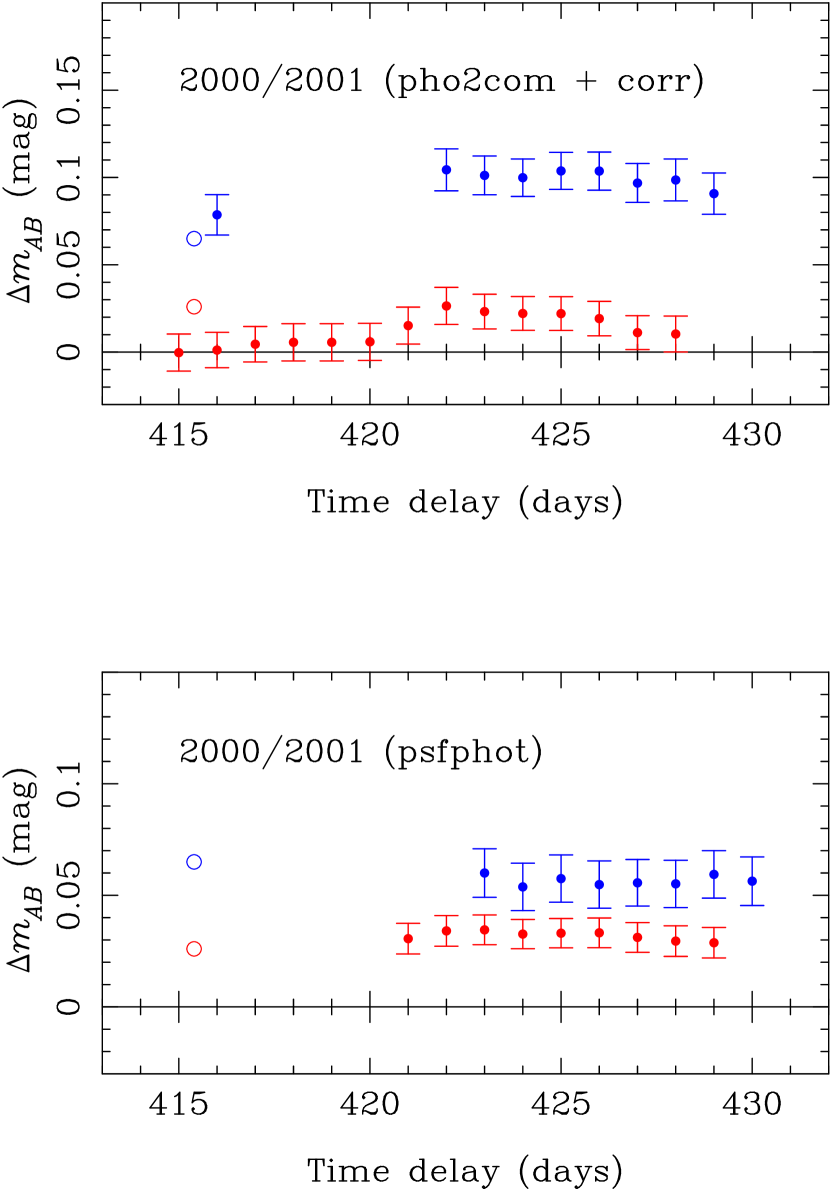
Figure 1: QSO 0957+561 magnification ratios in 2000 (2000/2001 seasons). While the top panel contains the results from the photometric method pho2comC, the bottom panel includes the results from an alternative photometric task (psfphot). Blue and red points are associated with ratios in the $V$ and $R$ bands, respectively. The filled circles are our measurements and the open circles are the typical estimates by the Oslo group (they did not use pho2comC or psfphot, but a different task). We are able to find ratios for time delays different to 415–416 days. In particular, the 420–430 days interval is very well tested.

From the GLITP brightness records of Q0957+561A and the about 14 months delayed Q0957+561B fluxes, one can find the $V$–band and $R$–band magnification ratios. Thus, first, we take the Q0957+561A fluxes in Figs. (6–7) of Ullán et al. (2003). These fluxes were derived from two photometric approaches: pho2com and psfphot, which led to two datasets consistent each other. Second, using the pho2com task, the subtraction of the lens galaxy in the Q0957+561B region is not perfect, and some additional correction must be incorporated (Serra-Ricart et al. 1999). Ullán et al. presented GLITP correction laws that qualitatively agree with contamination trends for the IAC–80 telescope/camera (operated in the Teide Observatory by the Instituto de Astrofisica de Canarias), so we use the pho2com method and the GLITP contamination laws to extract clean fluxes of Q0957+561B on 2001 April 10 (at the time $t_{B}$). The combined technique (pho2com + corr) is called pho2comC. Third, we obtain the fluxes of Q0957+561B at $t_{B}$ through the psfphot task. In this photometric technique, the way to determine the brightnesses of the two quasar components and the lens galaxy is from PSF fitting. We use the code developed and described by McLeod et al. (1998), which was kindly provided us. Several details on the psfphot approach were included in section 2 of that paper. The $V$–band (blue filled circles) and $R$–band (red filled circles) ratios are presented in Figure 1. While the top panel contains the results from pho2comC, the bottom panel includes the psfphot results. The $\Delta m_{AB}$ differences are computed in a simple way: given an optical filter, a task and a time delay $\Delta t_{AB}$, we compare the Q0957+561A data in a 5–days bin centered on $t_{B}-\Delta t_{AB}$ and the Q0957+561B flux at $t_{B}$. Only relatively populated bins are taken into account, i.e., bins with 3 or more data. It is a clear matter that the $\Delta m_{AB}(\lambda_{V},{\rm 2000})=\Delta m_{AB}(\lambda_{V})$ and $\Delta m_{AB}(\lambda_{R},{\rm 2000})=\Delta m_{AB}(\lambda_{R})$ are not similar. In other words, given a photometric approach and a time delay, the magnification ratios are not achromatic, and it is apparent the existence of a correlation between the ratios and the corresponding wavelengths, with the higher ratio for the smaller wavelength.

However, as we only have one frame in both filters ($V$ and $R$) at $t_{B}$, the $VR$ fluxes of Q0957+561B are not so well–determined as the free–of–peaks–of–noise and binned fluxes of Q0957+561A. Due to this fact, there is a small discrepancy between the $VR$ ratios from the two photometries. Fortunately, Ovaldsen et al. (2003b) reported $VR$ fluxes of QSO 0957+561 through five nights (one in 2000 January and four in 2001 March) of intensive monitoring at the NOT. The Oslo group used the same telescope in the same seasons, although they reduced the frames from another method (different to pho2comC or psfphot) and only tested the $VR$ magnification ratios for a delay of about 416 days. Their typical values $\Delta m_{AB}(\lambda_{V})$ = 0.065 mag (blue open circles in Fig. 1) and $\Delta m_{AB}(\lambda_{R})$ = 0.026 mag (red open circles in Fig. 1) agree with our results, and roughly represent a gap larger than the gap associated with psfphot, but smaller than the pho2comC gap. Once we confirm the absence of strongly biased results, as the $VR$ estimates for a given photometry do not seem to be very sensitive to the delay value, we introduce delay–averaged $VR$ ratios. In this first step, the effective ratios are: $\Delta m_{AB}(\lambda_{V})$ = 0.097 $\pm$ 0.011 mag and $\Delta m_{AB}(\lambda_{R})$ = 0.012 $\pm$ 0.010 mag, and $\Delta m_{AB}(\lambda_{V})$ = 0.057 $\pm$ 0.011 mag and $\Delta m_{AB}(\lambda_{R})$ = 0.032 $\pm$ 0.007 mag, from pho2comC and psfphot, respectively. The effective measurements are obtained from the averages of the typical values and errors for the different delays. In a second step, taking into account the estimates from the two photometric techniques, we infer the final global measurements. These $VR$ measurements are: $\Delta m_{AB}(\lambda_{V})$ = 0.077 $\pm$ 0.023 mag and $\Delta m_{AB}(\lambda_{R})$ = 0.022 $\pm$ 0.013 mag (1$\sigma$ intervals). Each 1$\sigma$ interval accounts for both the scatter between the typical values and the formal uncertainty of the photometric methods. The two individual contributions are added in quadrature.

3 Dust system

We are going to discuss the feasibility of two physical scenarios, which are usually introduced to explain optical ratios in disagreement with the expected macrolens ratio. The relative extinction of Q0957+561A is our first option. This relative extinction may be caused by dust in an intervening system. What system?. As the Milky Way is a bad candidate (the psfphot measurements and a hypothetical dust system at $z$ = 0 lead to unphysical extinction parameters), one can discard the differential extinction inside the Galaxy. However, in QSO 0957+561, we have four more candidates. Lens galaxies can generate differential extinction between the components of lensed quasars (e.g., Falco et al. 1999, Motta et al. 2002). Thus, the $z$ = 0.36 lens galaxy is an obvious candidate. It was discovered by Stockton (1980), and it is a giant elliptical galaxy residing in a cluster of galaxies. The light related to the A component and the light associated with the B component cross over two galaxy regions that are separated by $\sim$ 20 $h^{-1}$ kpc, where the Hubble constant is given by $H$ = 100 $h$ km s^-1 Mpc^-1, $\Omega$ = 0.3, and $\Lambda$ = 0.7. Besides the lens galaxy, there are two Ly absorption-line systems at redshifts $z$ = 1.1249 and $z$ = 1.3911 (e.g., Michalitsianos et al. 1997). The object closer to the observer ($z$ = 1.1249) is a Lyman limit system. For this system, spectra of QSO 0957+561 showed that the absorption in component A is marginally greater compared with component B. Therefore, assuming that more gas implies more dust, a relative extinction of Q0957+561A could be produced at $z$ = 1.1249. Michalitsianos et al. (1997) did a detailed study of the damped Ly $\alpha$ system at $z$ = 1.3911. In this far object, there is a strong evidence for different H I column densities between the lensed components, with the line of sight to image A intersecting a larger column density. The result $N_{A}$(H I) $>$ $N_{B}$(H I) was also claimed by Zuo et al. (1997), who suggested the possibility of a differential reddening by dust grains in the damped Ly $\alpha$ absorber. At $z$ = 1.3911, the ray paths of the lensed images are separated by $\approx$ 160 $h^{-1}$ pc (the separation between the ray paths is estimated from the scheme by Smette et al. 1992, but using an $\Omega$ = 0.3 and $\Lambda$ = 0.7 cosmology). Apart from the lens galaxy and the Ly absorption–line systems, one can also consider the source’s host galaxy at $z$ = 1.41.

Neglecting gravitational microlensing effects and assuming $R_{V}$–dependent Cardelli, Clayton, & Mathis (1989) extinction laws which are identical for both components, the dusty scenario leads to

$$\Delta m_{AB}(\lambda)=\Delta m_{AB}(\infty)+\Delta E(B-V)[a(x)R_{V}+b(x)],$$ (1)

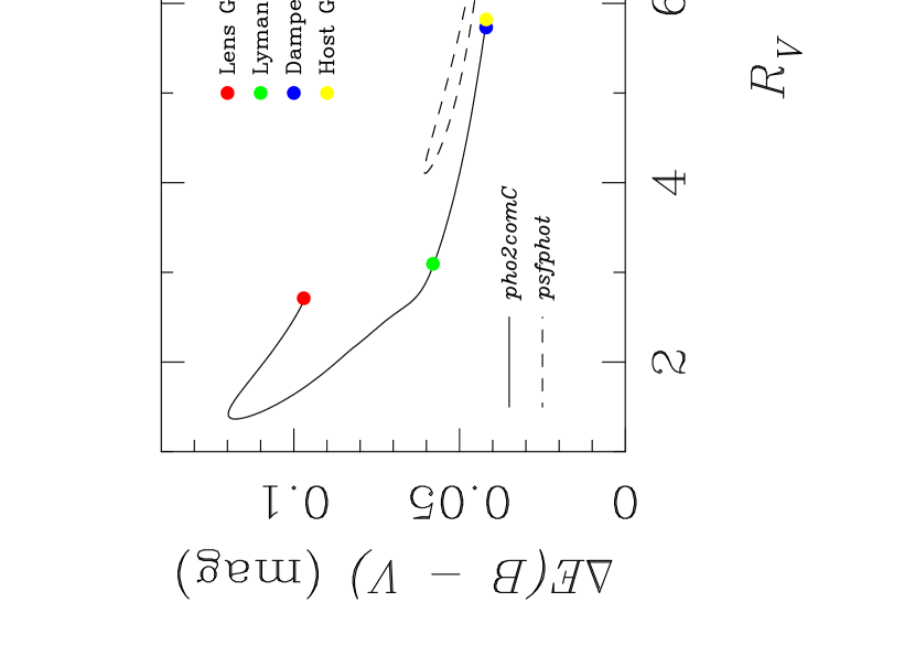
Figure 2: $\Delta E(B-V)$ and $R_{V}$ extinction parameters for dusty objects at 0.36 $\leq z_{dust}\leq$ 1.41. The solid line represents the parameters from the typical delay-averaged pho2comC ratios, whereas the dashed line traces the parameters from the typical delay-averaged psfphot ratios. The red points are the solutions for a dust system within the lens galaxy ($z_{dust}$ = 0.36), the green points represent the solutions for $z_{dust}$ = 1.1249 (Lyman limit system), the blue points are related to a dusty damped object ($z_{dust}$ = 1.3911), and the yellow points are associated with a dusty host galaxy ($z_{dust}$ = 1.41).

where $\Delta m_{AB}(\infty)$ is the macrolens ratio or the ratio at $\lambda=\infty$ (in our case, $\Delta m_{AB}(\infty)=-$ 0.31 mag; see Introduction), and $\Delta E(B-V)$ is the differential extinction. Here, $R_{V}=A_{V}/E(B-V)$ is the ratio of total to selective extinction in the $V$ band, and $a(x)$ and $b(x)$ are known functions of $x=(1+z_{dust})/\lambda$ (Cardelli et al. 1989). We take the typical delay–averaged $VR$ magnification ratios from pho2comC and psfphot, which are considered as two extreme cases: a big gap of 0.085 mag (pho2comC) and a small gap of 0.025 mag (psfphot). The Ovaldsen et al.’s measurement would correspond to an intermediate case of $\Delta m_{AB}(\lambda_{V})-\Delta m_{AB}(\lambda_{R})\approx$ 0.040 mag. For each photometry, we estimate the two extinction parameters, $\Delta E(B-V)$ and $R_{V}$, as a function of the redshift of an intervening object, $z_{dust}$. The results are showed in Figure 2. The solid line represents the extinction parameters from the pho2comC ratios, whereas the dashed line traces the parameters from the psfphot ratios. In Fig. 2, the red points are the solutions for $z_{dust}$ = 0.36 (lens galaxy), the green points are the solutions for $z_{dust}$ = 1.1249 (Lyman limit system), the blue points are associated with $z_{dust}$ = 1.3911 (damped Ly $\alpha$ system), and the yellow points are associated with $z_{dust}$ = 1.41 (host galaxy). If we focus on the four candidates (lens galaxy, Ly absorption–line systems, and QSO’s host galaxy), global intervals $\Delta E(B-V)$ = 0.03–0.10 mag and $R_{V}$ = 2–9 are derived. In the Galaxy, typical paths have a ratio of total to selective extinction $R_{V}\approx$ 3.1, while paths through typical and non–typical extinction regions have values in the range 2–6. The $R_{V}$ values in far galaxies can be even higher. For example, the $z$ = 0.68 spiral lens B0218+357 has $R_{V}\approx$ 7–12 (Falco et al. 1999; Muñoz et al. 2004). Therefore, the results on $R_{V}$ seem reasonable. On the other hand, the range for differential extinction agrees with typical values in lens systems, and as a general conclusion, the observations can be explained by means of a dusty scenario.

How is the structure of the dust system?. The ray paths of the two components cross either different environments (i.e., B crosses an empty zone and A crosses a dusty zone) or the same dusty environment. In the first case, as the emission–lines sources do not experience (important) differential extinction and the optical continuum compact sources suffer it, the A zone would include a compact dust cloud in the trajectory of the A beam together with a random distribution of similar clumps of dust. The distribution of clouds cannot significantly perturb the radiation from the emission–lines sources. If the projected (into the source plane) cloud radius is $R_{cloud}$ = 0.01 pc, i.e., similar to the expected radial size of the whole accretion disk around a 10⁸ M_⊙ black hole, then the time of cloud crossing by the optical continuum region (OCR) is of about 30 years (considering $R_{OCR}<R_{cloud}$ and an effective transverse velocity of 600 km s^-1; e.g., Wambsganss et al. 2000). If we also consider the existence of $N$ dust clouds in front of the broad–line region (BLR) as well as a typical radius $R_{BLR}$ = 0.1 pc, the surface covering factor of the dust would be $f_{dust/BLR}=N(R_{cloud}/R_{BLR})^{2}=10^{-2}N$. As $f_{dust/BLR}$ should be much smaller than 1 ($f_{dust/BLR}<<$ 1), a constraint on the surface density of clouds can be derived in a simple way. It must be much smaller than 10⁴/$\pi$ clouds pc^-2, so the probability to see a cloud crossing phenomenon is equal to or less than 10%. The situation is better in the second case, when the A and B zones are within the same environment. While a homogeneous distribution of dust is not consistent with the optical continuum ratios, an inhomogeneous distribution works well. We assume an environment constituted by a network of compact dust clouds and compact empty regions ($R_{cloud}$ = $R_{void}$ = 0.01 pc), with a cloud in the trajectory of the A beam and a void in the trajectory of the other (B) beam. In this picture, the optical continuum ratios would be anomalous, but the emission–line ratios would be very close to the macrolens ratio, because two large regions contain a very similar amount of dust. Moreover, both the probability of a cloud crossing (component A) and the probability of a void crossing (component B) are of about 50%. Hence, the probability of a cloud(A)/void(B) crossing is crudely of 25%. For the farest candidate (host galaxy), the common environment is a very reasonable approach, and for the nearest candidate (lens galaxy), the common environment could be due to the presence of an inhomogeneous dust lane with a length of $\geq$ 20 kpc.

4 Microlensing

To explain the chromatic ratios, the gravitational microlensing of QSO 0957+561 is our second option. While the emission-lines regions are not magnified from gravitational microlensing, the optical continuum compact sources could be affected by this physical phenomenon. Using the values for the normalized surface mass density (convergence) and the shear, we produce 2–dimensional magnification maps with a ray shooting technique (Wambsganss 1990, 1999). These values are: $\kappa_{A}$ = 0.22, $\gamma_{A}$ = 0.17, $\kappa_{B}$ = 1.24, and $\gamma_{B}$ = 0.9 (Pelt et al. 1998). With respect to the fraction of the surface mass density represented by the microlenses, we consider three cases: (a) all the mass is assumed to be in granular form (compact objects), (b) 50% of the mass in granular form, and (c) the mass is dominated by a smoothly distributed material, with only 25% of the mass in compact objects. All the microlensing objects are assumed to have a similar mass $M$ and are distributed randomly over the lens plane. We obtain detailed results for $M=1M_{\odot}$, and comment the expected results for smaller masses ($M<1M_{\odot}$). The effect of the source is taken into account by convolving a selected source intensity profile with the magnification maps. We consider two different circularly–symmetric profiles: a $p$ = 3/2 power–law (PL) profile and a Gaussian (GS) profile. The PL profile was introduced by Shalyapin (2001), and it is roughly consistent with the standard accretion disk. The GS profile is not so smooth as the PL one, and it was used in almost all previous microlensing studies in QSO 0957+561. In our model we assume that the $V$–band source has a characteristic length (intensity distribution) of $R_{V}$ = 3 $\times$ 10¹⁴ cm (small source), $R_{V}$ = 10¹⁵ cm (intermediate source), or $R_{V}$ = 3 $\times$ 10¹⁵ cm (large source), and the source size ratio $q=R_{V}/R_{R}$ is given by about 0.8 or 1/3. For the standard accretion disk model, one has the relationship $R(\lambda)\propto\lambda^{4/3}$ (e.g., Shalyapin et al. 2002), and consequently, the standard ratio $q\approx$ 0.8, which is close to the critical ratio ($q$ = 1). It is also assumed that the source, the deflector and the observer are embedded in a standard flat cosmology: $H$ = 100 $h$ km s^-1 Mpc^-1, $h$ = 2/3, $\Omega$ = 0.3, $\Lambda$ = 0.7.

In other recent analyses about QSO 0957+561 microlensing (Refsdal et al. 2000; Wambsganss et al. 2000), the authors concentrated on the time evolution of $\Delta m_{AB}$ in a given optical band. Refsdal et al. (2000) used a GS source and found 90% confidence level constraints for the microlenses mass $M$ and the source radius $R$: $M$ = 2 $\times$ 10^-3 – 0.5 $M_{\odot}$, $R<$ 6 $\times$ 10¹⁵ cm. On the other hand, Wambsganss et al. (2000) claimed that the microlenses mass must be $\geq$ 0.1 $M_{\odot}$ for small GS sources (3$\sigma$ limit). All these previous constraints are based on the hypothesis of a Gaussian source, and moreover, as the analyses were focused on the time domain, some hypotheses about both the effective transverse velocity and the random microlens motion were needed. However, our approach is different, because we wish to study the spectral evolution of $\Delta m_{AB}$ at a given emission time. In this paper, we discuss both the GS and PL profiles and do not need to introduce a dynamical hypothesis. In fact, in relation to multiepoch simulations, multiband simulations have the advantage of being free from assumptions on the peculiar motions of the quasar and deflector, and the orbits of the microlenses in the lens galaxy and cluster centre.

The key idea is that the $VR$ magnification ratios are generated by two circular concentric sources with different size. The common center of the $V$–band and $R$–band sources is placed at two arbitrary pixels of the two magnification patterns, and we look for the corresponding [$\Delta m_{AB}(\lambda_{V})$,$\Delta m_{AB}(\lambda_{R})$] pair. For a given set of physical parameters, we can test a very large number of pairs of pixels (10⁴), and thus, obtain a distribution of pairs of magnification ratios. In the [$\Delta m_{AB}(\lambda_{V})$,$\Delta m_{AB}(\lambda_{R})$] plane, for $q$ = 1 (critical source size ratio), the simulated distributions would lie exactly on the $\Delta m_{AB}(\lambda_{R})$ = $\Delta m_{AB}(\lambda_{V})$ straight line (critical line). However, when $q\neq$ 1, we must infer 2D distributions, including points at non-zero distances (in magnitudes) from the critical line. The 2D distributions in the six panels of Fig. 3 have been derived by using a deflector with only granular matter ($M=1M_{\odot}$) and GS sources. In Fig. 3 (and also Fig.4), the results for the small, intermediate and large $V$–band sources are depicted in the top, middle and bottom panels, respectively. The left panels correspond to a standard $q$, and the right panels correspond to a non–standard $q$ ($q$ = 1/3). We also draw the rectangle associated with the 1$\sigma$ measurements. It is apparent that larger differences between $R_{V}$ and $R_{R}$ imply wider distributions. In Fig. 3, we only see a very interesting region of the whole plane, which includes the observed magnification ratios. The reader can extrapolate the six behaviours in this region towards a larger region along and around the critical line. In order to get a good resolution, instead of the whole 2D distributions, we decided in favour of a smaller (but representative) region. What about the PL intensity profile?. In Fig. 4, we again consider all the mass in compact objects of $M=1M_{\odot}$, but PL sources. The new distributions are different to their partners in Fig. 3 (with similar values of $R_{V}$ and $R_{R}$). However, for obtaining quantitative conclusions, some additional analyses are needful.

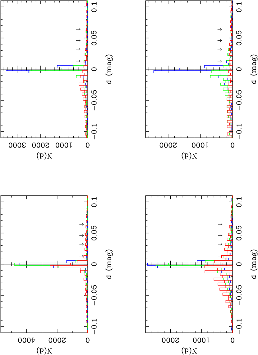
Figure 5: Histograms $N(d)$ for the scenarios with 100% of the mass in compact objects ($M=1M_{\odot}$). For a given set of physical parameters, we infer a distribution of 10⁴ points in the [$\Delta m_{AB}(\lambda_{V})$,$\Delta m_{AB}(\lambda_{R})$] plane. In a second step, we obtain the number of points at different distances $d$ (in magnitudes) from the critical line $\Delta m_{AB}(\lambda_{R})=\Delta m_{AB}(\lambda_{V})$. The distribution $N(d)$ is computed for points above the critical line ($d<$ 0) and below the critical line ($d>$ 0). The results from Gaussian sources and a standard source size ratio ($\approx$ 0.8), Gaussian sources and a non–standard $q$ (= 1/3), $p$ = 3/2 power–law sources and a standard $q$, and $p$ = 3/2 power–law sources and a non–standard $q$ appear in the top left panel, the top right panel, the bottom left panel, and the bottom right panel, respectively. We use blue lines for $R_{V}$ = 3 $\times$ 10¹⁴ cm, green lines for $R_{V}$ = 10¹⁵ cm, and red lines for $R_{V}$ = 3 $\times$ 10¹⁵ cm. The four arrows indicate the distances from the critical line to the four vertexes of the 1$\sigma$ rectangle in Figs. 3 and 4.

We make 12 histograms $N(d)$ for the 12 scenarios where 100% of the mass is contained in compact objects ($M=1M_{\odot}$). Each histogram represents the number of points at different distances $d$ (in magnitudes) from the critical line. Given the [$\Delta m_{AB}(\lambda_{V})$,$\Delta m_{AB}(\lambda_{R})$] pair, the distance from the critical line, $d=[\Delta m_{AB}(\lambda_{V})-\Delta m_{AB}(\lambda_{R})]/\sqrt{2}$, and the difference between ratios, $D=\Delta m_{AB}(\lambda_{V})-\Delta m_{AB}(\lambda_{R})$, differ only in a factor $\sqrt{2}$. Therefore, we analyze histograms $N(d)$, which are basically $D$ distributions. The points above the critical line have negative distances ($d<$ 0), whereas the points below the critical line have positive distances ($d>$ 0). All the histograms are showed in Fig. 5: GS profile and standard $q$ (top left panel), GS profile and $q$ = 1/3 (top right panel), PL profile and standard $q$ (bottom left panel), and PL profile and $q$ = 1/3 (bottom right panel). We use blue lines for the small $V$–band source, green lines for the intermediate $V$–band source, and red lines for the large $V$–band source. The four arrows indicate the distances from the critical line to the four vertexes of the 1$\sigma$ rectangle in Figs. 3 and 4. If the true [$\Delta m_{AB}(\lambda_{V})$,$\Delta m_{AB}(\lambda_{R})$] pair would be within the 1$\sigma$ box, then the true distance would verify $d\geq$ 0.013 mag. Here, we assume that the true pair is placed at $d\geq$ 0.013 mag, so probabilities $P$($d<$ 0.013 mag) are computed. Some probability distributions (histograms) lead to very high values of $P$($d<$ 0.013 mag), and thus, we can rule out the corresponding scenarios. On the contrary, other $N-d$ relationships are relatively consistent with the constraint. The estimates of $P$($d<$ 0.013 mag) appear in Table 1, and we see several values $\leq$ 90%, which suggest realistic physical parameters, or in other words, viable scenarios. In the GS profile case, the feasible pictures are related to either the large $V$–band source or an intermediate $V$–band source together with a non–standard $R$–band companion. In the PL profile case, from the $P\leq$ 90% criterion, all the scenarios seem to be plausible.

In Fig. 6, we see the magnification maps for the Q0957+561A (left panel) and Q0957+561B (right panel) components as well as the 10000 pairs of pixels (white marks) used to produce Figs. 3, 4 and 5. For the B component, the granular mass density is high and the caustic network almost takes up the whole map. The 10⁴ highlighted pixels in each map are randomly distributed, so the sampling is not biased. In Fig. 7, the chromatic microlensing is apparent. The caustic maps in Fig. 6 are convolved with the largest Gaussian sources ($R_{V}$ = 3 $\times$ 10¹⁵ cm, $R_{R}$ = 3 $\times$ $R_{V}$). In the three top panels of Fig. 7, we include the $V$–convolved map for the A component (left), the $R$–convolved map for the A component (centre), and the difference between the two convolutions (right). The results for the B component appear in the three bottom panels of Fig. 7: $V$–convolution (left), $R$–convolution (centre), and difference (right). It is clear that the convolutions with the $V$–band source are different to the convolutions with the $R$–band source. This fact gives rise to the appearance of chromatic effects, i.e., there are difference signals in the two right panels.

When all the mass is not contained in compact objects, i.e., a certain mass fraction is smoothly distributed, we can repeat the above–mentioned procedure and obtain new 2D distributions, histograms, probabilities, etc. To avoid an ”excess of complementary material” (figures), only the $P$($d<$ 0.013 mag) values are included in Table 1. Two different cases are analyzed in this paper: 50% of the mass in granular form (50% of the mass in a smoothly distributed component), and 25% of the mass in compact objects (75% of the mass is contained in a smoothly distributed material). As the percentage of mass in compact objects decreases, it is more difficult to find scenarios in agreement with the observational constraint. In fact, when the mass is dominated by a smoothly distributed material, almost all the physical pictures are ruled out by the observations at the 90% level. Only two rare scenarios (where the source sizes are in a relation 1:3) lead to $P$($d<$ 0.013 mag) $\leq$ 90%, or equivalently, $P$($d\geq$ 0.013 mag) $>$ 10%. Although from a population of microlenses of $M=1M_{\odot}$ we are able to test an important set of physical situations, we must also think about the expected results from a population of microlenses of $M<1M_{\odot}$. In the extreme (but still plausible) case of $M=10^{-2}M_{\odot}$, the physical size of the magnification maps (the maps are 2048 pixels a side which cover a physical size of 16 Einstein radii) reduces in a factor 10 (just the factor that relates the Einstein radii for 1 $M_{\odot}$ and $10^{-2}M_{\odot}$). Now, the $V$–band and $R$–band sources with radii $R_{R}$ and $R_{V}$ work as the sources with radii 10 $\times R_{R}$ and 10 $\times R_{V}$ in the old case ($M=1M_{\odot}$). For example, the results in Table 1 for $R_{V}$ = 3 $\times$ 10¹⁵ cm would be the results for $R_{V}$ = 3 $\times$ 10¹⁴ cm and $M=10^{-2}M_{\odot}$.

We remark that the discussion is based on arrays of 2048 by 2048 pixels, which cover 16 $R_{E}$ $\times$ 16 $R_{E}$ regions. Similar arrays were used by Schmidt & Wambsganss (1998) in the cases $M\geq 10^{-2}M_{\odot}$, and we think that our results are reliable. However, in very detailed studies to discriminate between different microlensing pictures, magnification maps with larger spatial coverage and better spatial resolution may be useful. Some of these improvements are related to the availability of high performance computers.

5 Conclusions and future work

We present in this work a very robust estimation of the $VR$ magnification ratios of QSO 0957+561. The new measurements are based on observations (in 2000–2001) with the 2.56m Nordic Optical Telescope, two different photometric techniques, and a reasonable interval for the time delay in the system. Our 1$\sigma$ estimates $\Delta m_{AB}(\lambda_{V})$ = 0.077 $\pm$ 0.023 mag and $\Delta m_{AB}(\lambda_{R})$ = 0.022 $\pm$ 0.013 mag are supported by the results in Ovaldsen et al. (2003b). A first conclusion is the relation $\Delta m_{AB}(\lambda_{V})>\Delta m_{AB}(\lambda_{R})$, which means that the optical continuum magnification ratios are not achromatic, and moreover, the higher ratio corresponds to the smaller wavelength.

To explain the measurements, two alternatives are explored: a dust system between the quasar and the observer, or a population of microlenses in the deflector (the most popular picture). We find that the observed ratios are consistent with both alternatives, i.e., differential extinction in a dust system and gravitational microlensing in the deflector. We cannot rule out the existence of a dusty scenario constituted by a network of compact dust clouds and compact empty regions, with a cloud in the line of sight to the Q0957+561A component and a void in the trajectory of the Q0957+561B beam. The new estimates cover a narrow spectral range (0.536–0.645 $\mu$m), and this fact plays a dramatic role in the discrimination of possible physical scenarios. We think that future accurate measurements at a large collection of wavelengths, with a good coverage of the 0.2–1 $\mu$m range, will decide on the feasibility of a dust system in QSO 0957+561 and other things. For example, the GTC (a segmented 10.4 meter telescope to be installed in one of the best sites of the Northern Hemisphere: the Roque de los Muchachos Observatory, La Palma, Canary Islands, Spain. First light is planed for 2005) will have an instrument (OSIRIS) with very interesting preformances. OSIRIS will incorporate tunable filters with FWHM from 10^-4 to 7 $\times$ 10^-3 $\mu$m over the whole optical wavelength range, and thus, tunable imaging of the two quasar components at two epochs (separated by the time delay) could lead to solve the current puzzle (dust or microlenses?) and infer tight constraints on the physical parameters of the favoured alternative. Observations in the ultraviolet wavelength range ($\leq 0.36\mu$m) may also be a decisive tool. In particular, if the actual origin of the magnification ratio anomalies is a dust system in the lens galaxy.

If the 0.2175 $\mu$m extinction bump would be unambiguously detected (assuming dusty scenarios in the 0.36–1.41 redshift interval, the rest-frame wavelength of the peak corresponds to 0.30–0.52 $\mu$m in the observer frame), then the current extinction/microlensing degeneration would be broken. In this last case (detection of extinction), one may try to derive a very rich information: the differential extinction, the ratio of total to selective extinction in the $V$ band, the macrolens ratio, the redshift of the dust, and so on (e.g., Falco et al. 1999). On the other hand, if the dusty scenarios would be ruled out from future observations at lots of wavelengths, the multiwavelength ratios may be used to decide on the viable gravitational microlensing scenarios. From a simple analysis, we show that several microlensing scenarios are ruled out by the new observations at the 90% level (see Table 1 and Sect. 4), so future detailed data could lead to important constraints. The future observational work will require new ingredients in the microlensing scheme, e.g., new source intensity profiles (in particular, the standard accretion disk profile; Shalyapin et al. 2002), or a two mass population of microlenses, describing the granular matter in the lens galaxy and the granular matter in the cluster centre (e.g., Schechter, Wambsganss & Lewis 2004). Sophisticated source models could be also included. The double ring structure suggested by Schild & Vakulik (2003) is an obvious candidate. These authors have described the $R$–band source, but they did not quote the chromatic behaviour of the five model parameters: the radius of the large ring, the radial thickness of the large ring, the radius of the small ring, the thickness of the small ring, and the brightness ratio of the two rings, which is a basic issue to simulate multiwavelength magnification ratios. The extinction and microlensing hypotheses can be tested in both the frequency and time domains, and several previous efforts focused on the possible microlensing variability (e.g., Refsdal et al. 2000; Wambsganss et al. 2000). Obviously, the observations in the time domain (evolution of the magnification ratios) have a great interest. However, when they are compared to microlensing simulations, the microlensing framework must incorporate dynamical information, i.e., the confrontation between the observed evolution and the microlensing scheme requires additional free parameters (which are needless in multiwavelength studies). Finally, we note that the two alternative schemes (only dust or only microlenses) might be biased models of the actual situation, and a mixed scenario (extinction + microlensing) is also possible. Very recently, to explain spectrophotometric observations of the lens system HE 0512$-$3329, Wucknitz et al. (2003) proposed this mixed model.

Table 1: Probabilities for measuring a pair of magnification ratios (one in the $V$ band and the other in the $R$ band) at a distance $<$ 0.013 magnitudes from the critical line $\Delta m_{AB}(\lambda_{R})$ = $\Delta m_{AB}(\lambda_{V})$.

Mass in granular form (%)	Intensity profile	$R_{V}$ (cm)	$q=R_{V}/R_{R}$	$P$($d<$ 0.013 mag) (%)	$P\leq$ 90%?
100	Gaussian	3 $\times$ 1014	$\approx$ 0.8	93.5	–
			1/3	91.4	–
		1015	$\approx$ 0.8	91.1	–
			1/3	81.7	yes
		3 $\times$ 1015	$\approx$ 0.8	80.0	yes
			1/3	68.6	yes
	Power–law ($p$ = 3/2)	3 $\times$ 1014	$\approx$ 0.8	89.1	yes
			1/3	85.5	yes
		1015	$\approx$ 0.8	86.6	yes
			1/3	75.3	yes
		3 $\times$ 1015	$\approx$ 0.8	78.2	yes
			1/3	69.0	yes
50	Gaussian	3 $\times$ 1014	$\approx$ 0.8	97.9	–
			1/3	96.5	–
		1015	$\approx$ 0.8	96.8	–
			1/3	90.8	–
		3 $\times$ 1015	$\approx$ 0.8	91.3	–
			1/3	80.4	yes
	Power–law ($p$ = 3/2)	3 $\times$ 1014	$\approx$ 0.8	95.6	–
			1/3	93.1	–
		1015	$\approx$ 0.8	93.9	–
			1/3	84.7	yes
		3 $\times$ 1015	$\approx$ 0.8	85.9	yes
			1/3	75.8	yes
25	Gaussian	3 $\times$ 1014	$\approx$ 0.8	99.3	–
			1/3	99.0	–
		1015	$\approx$ 0.8	98.8	–
			1/3	96.6	–
		3 $\times$ 1015	$\approx$ 0.8	95.8	–
			1/3	89.4	yes
	Power–law ($p$ = 3/2)	3 $\times$ 1014	$\approx$ 0.8	98.2	–
			1/3	97.2	–
		1015	$\approx$ 0.8	97.7	–
			1/3	92.5	–
		3 $\times$ 1015	$\approx$ 0.8	92.3	–
			1/3	80.8	yes

Figure 3: Synthetic distributions of [$\Delta m_{AB}(\lambda_{V})$,$\Delta m_{AB}(\lambda_{R})$] pairs for a deflector with only granular matter ($M=1M_{\odot}$) and Gaussian sources. The radii of the $V$–band sources are $R_{V}$ = 3 $\times$ 10¹⁴ cm (top panels), $R_{V}$ = 10¹⁵ cm (middle panels), and $R_{V}$ = 3 $\times$ 10¹⁵ cm (bottom panels). In the left panels, we consider a standard $q=R_{V}/R_{R}$ of about 0.8, and in the right panels, we take a non–standard source size ratio of $q$ = 1/3. The 1$\sigma$ measurements in this paper are also depicted in each panel (small rectangle). A few simulated pairs are within the 1$\sigma$ rectangle, so they are fully consistent with the observations. However, we generate 10⁴ pairs for each physical picture, with the vast majority of points out of the observational box, and even out of the $-0.15\leq\Delta m_{AB}(\lambda_{V})$ (in mag) $\leq 0.15$ and $-0.15\leq\Delta m_{AB}(\lambda_{R})$ (in mag) $\leq 0.15$ region.

Figure 4: Synthetic distributions of [$\Delta m_{AB}(\lambda_{V})$,$\Delta m_{AB}(\lambda_{R})$] pairs for a deflector with only granular matter ($M=1M_{\odot}$) and $p$ = 3/2 power–law sources. See the caption in Fig. 3 for comments on the six panels.

Figure 6: Details on the caustic maps and the locations of the 10⁴ pairs of pixels used to produce Figs. 3–5. The selected pairs of pixels (white marks) are randomly distributed within the magnification maps for the A (left panel) and B (right panel) components.

Figure 7: Example of chromatic microlensing. We use the magnification maps in Fig. 6 and the largest GS sources ($R_{V}$ = 3 $\times$ 10¹⁵ cm, $R_{R}$ = 3 $\times$ $R_{V}$). The convolved maps for the A component appear in the top panels: $V$–convolution (left), $R$–convolution (centre), and difference between both convolutions (right). On the other hand, the convolved maps for the B component are depicted in the bottom panels: $V$–convolution (left), $R$–convolution (centre), and difference (right). The difference signals have a structure that is correlated to the structure of the caustic networks.

References

- (1) Cardelli, J. A., Clayton, G. C., & Mathis, J. S. 1989, ApJ, 345, 245
- (2) Conner, S. R., Lehár, J., & Burke, B. F. 1992, ApJ, 387, L61
- (3) Falco, E. E., Impey, C. D., Kochanek, C. S., Lehár, J., McLeod, B. A., Rix, H.-W., Keeton, C. R., Muñoz, J. A., & Peng, C. Y. 1999, ApJ, 523, 617
- (4) Garrett, M. A., Calder, R. J., Porcas, R. W., King, L. J., Walsh, D., & Wilkinson, P. N. 1994, MNRAS, 270, 457
- (5) Kundić, T., Turner, E. L., Colley, W. N., Gott III, J. R., Rhoads, J. E., Wang, Y., Bergeron, L. E., Gloria, K. A., Long, D. C, Malhotra, S., & Wambsganss, J. 1997, ApJ, 482, 75
- (6) McLeod, B. A., Bernstein, G. M., Rieke, M. J., & Weedman, D. W. 1998, AJ, 115, 1377
- (7) Michalitsianos, A. G., Dolan, J. F., Kazanas, D., Bruhweiler, F. C., Boyd, P. T., Hill, R. J., Nelson, M. J., Percival, J. W., & van Citters, G. W. 1997, ApJ, 474, 598
- (8) Motta, V., Mediavilla, E., Muñoz, J. A., Falco, E., Kochanek, C. S., Garcia–Lorenzo, B., Oscoz, A., & Serra–Ricart, M. 2002, ApJ, 574, 719
- (9) Muñoz, J. A., Falco, E. E., Kochanek, C. S., McLeod, B. A., & Mediavilla, E. 2004, ApJ, 605, 614
- (10) Oscoz, A., Alcalde, D., Serra–Ricart, M., Mediavilla, E., & Muñoz, J. A. 2002, ApJ, 573, L1
- (11) Ovaldsen, J. E., Teuber, J., Schild, R. E., & Stabell, R. 2003a, A&A, 402, 891
- (12) Ovaldsen, J. E., Teuber, J., Stabell, R., & Evans, A. K. D. 2003b, MNRAS, 345, 795
- (13) Pelt, J., Schild, R., Refsdal, S., & Stabell, R. 1998, A&A, 336, 829
- (14) Press, W. H., & Rybicki, G. B. 1998, ApJ, 507, 108
- (15) Refsdal, S., Stabell, R., Pelt, J., & Schild, R. 2000, A&A, 360, 10
- (16) Schechter, P. L., Wambsganss, J., & Lewis, G. F. 2004, astro-ph/0403558
- (17) Schild, R. E., & Smith, R. C. 1991, AJ, 101, 813
- (18) Schild, R., & Vakulik, V. 2003, AJ, 126, 689
- (19) Schmidt, R., & Wambsganss, J. 1998, A&A, 335, 379
- (20) Serra–Ricart, M., Oscoz A., Sanchís, T., Mediavilla, E., Goicoechea, L. J., Licandro, J., Alcalde, D., & Gil–Merino, R. 1999, ApJ, 526, 40
- (21) Shalyapin, V. N. 2001, Astron. Lett., 27, 150
- (22) Shalyapin, V. N., Goicoechea, L.J., Alcalde, D., Mediavilla, E., Muñoz, J.A., & Gil–Merino, R. 2002, ApJ, 579, 127
- (23) Smette, A., Surdej, J., Shaver, P. A., Foltz, C. B., Chaffee, F. H., Weymann, R. J., Williams, R. E., & Magain, P. 1992, ApJ, 389, 39
- (24) Stockton, A. 1980, ApJ, 242, L141
- (25) Ullán, A., Goicoechea, L.J., Muñoz, J.A., Mediavilla, E., Serra–Ricart, M., Puga, E., Alcalde, D., Oscoz, A., & Barrena, R. 2003, MNRAS, 346, 415
- (26) Walsh, D., Carswell, R. F., & Weymann, R. J. 1979, Nature, 279, 381
- (27) Wambsganss, J. 1990, PhD thesis, Munich University (report MPA 550)
- (28) Wambsganss, J. 1999, Journ. Comp. Appl. Math., 109, 353
- (29) Wambsganss, J., Schmidt, R. W., Colley, W., Kundić, T., & Turner, E. L. 2000, A&A, 362, L37
- (30) Wucknitz, O., Wisotzki, L., Lopez, S., & Gregg, M. D. 2003, A&A, 405, 445
- (31) Zuo, L., Beaver, E. A., Burbidge, E. M., Cohen, R. D., Junkkarinen, V. T., & Lyons, R. W. 1997, ApJ, 477, 568