Variable stars in the bar of the Large Magellanic Cloud: the photometric catalogue

The catalogue of the Johnson-Cousins $B,V$ and $I$ light curves obtained for 162 variable stars (135 RR Lyrae, 4 candidate Anomalous Cepheids, 11 Classical Cepheids, 11 eclipsing binaries and 1 $\delta$ Scuti star) in two areas close to the bar of the Large Magellanic Cloud is presented along with coordinates, finding charts, periods, epochs, amplitudes, and mean quantities (intensity- and magnitude-averaged luminosities) of the variables with full coverage of the light variations. A star by star comparison is made with MACHO and OGLE II photometries based on both variable and constant stars in common, and the transformation relationships to our photometry are provided. The pulsation properties of the RR Lyrae stars in the sample are discussed in detail. Parameters of the Fourier decomposition of the light curves are derived for the fundamental mode RR Lyrae stars with complete and regular curves (29 stars). They are used to estimate metallicities, absolute magnitudes, intrinsic $(B-V)_{0}$ colours, and temperatures of the variable stars, according to Jurcsik and Kovács (1996), and Kovács and Walker (2001) method. Quantities derived from the Fourier parameters are compared with the corresponding observed quantities. In particular, the “photometric” metallicities are compared with the spectroscopic metal abundances derived by Gratton et al. (2004) from low resolution spectra obtained with FORS at the Very Large Telescope.

1 Introduction

RR Lyrae stars and Cepheids are primary distance indicators and set the astronomical distance scale to the Large Magellanic Cloud and to the galaxies of the Local Group. Being from 2 to 6-7 magnitudes brighter than the RR Lyrae stars, Cepheids allow to reach galaxies as far as $\simeq$ 20 Mpc (see Freedman et al. 2001). Conspicuous samples of these variables have been discovered in the Large Magellanic Cloud (LMC) as a by-product of the microlensing surveys conducted by the MACHO collaboration (Alcock et al. 1996, hereinafter A96) and by OGLE II (Udalski et al. 1997). A96 found more than 7,900 RR Lyrae stars in the $\sim$ 39,000 arcmin² of the LMC they surveyed, among which 181 double-mode pulsators (RRd’s, Alcock et al. 1997, 2000), as well as large numbers of Cepheids and eclipsing binary systems. Similar numbers are reported by OGLE II (Soszyński et al. 2003), who also increased to 230 the number of double-mode RR Lyrae stars. Calibrated photometry for the LMC RR Lyrae stars has been published by both the MACHO collaboration (Alcock et al. 2003a) and the OGLE II team (Soszyński et al. 2003). However, non-standard photometric passbands were used by MACHO, and the RR Lyrae stars are near the limiting magnitudes of these surveys, so that the photometric accuracy of the individual light curves is reduced. This limits the use of these samples in the derivation of very precise estimates of the LMC distance, or in the study and theoretical reproduction of the light curves (see for instance Marconi & Clementini 2004). Besides, in these experiments the variable stars were mainly observed in $V$ and $I$ and only to a lesser extent in the $B$ passband, thus limiting the comparison with most of the Galactic samples which instead generally use $B$ and $V$.

We have obtained accurate multiband time series photometry reaching $V\sim$ 23 (i.e. $\sim$ 3.5 mag fainter than the RR Lyrae stars in the LMC) of two 13${}^{\prime}\times 13^{\prime}$ fields close to the bar of the LMC and studied their variable stars (135 RR Lyrae, 4 candidate Anomalous Cepheids, 11 Classical Cepheids, 11 eclipsing binaries, and 1 $\delta$ Scuti). The photometric data were complemented by spectroscopic observations obtained with the 3.6 m and the VLT ESO telescopes in 1999 and 2001, respectively, and used to derive individual metallicities for 103 of the variables in the present sample, and the luminosity-metallicity relation (M${}_{V}(RR)-$ [Fe/H]) of the LMC RR Lyrae stars (Bragaglia et al. 2001, Clementini et al. 2003a, hereinafter C03, Gratton et al. 2004, hereinafter G04). A discussion of the astrophysical impact of the new data on the derivation of the $M_{V}(RR)-$[Fe/H] relationship and on the definition of the distance to the LMC has been presented in C03.

In this paper we present the catalogue of the $B,V,I$ light curves obtained for the 162 short period variables we have identified in the two fields. In Section 2 we describe the acquisition, reduction and calibration of the data. Section 3 describes the identification, the period search procedures and the characteristics of the variables. In Section 4 we present the star-by-star comparison with MACHO and OGLE II photometries, based on both variable and constant stars in common, and provide transformation relationships. The period distribution and the period amplitude relations followed by the RR Lyrae stars in our sample are discussed in Section 5. In Section 6 we discuss the metallicities, absolute magnitudes, intrinsic $(B-V)_{0}$ colours, and effective temperatures derived from the the Fourier decomposition of the light curve of the ab-type RR Lyrae stars with regular light curves (29 stars) and compare them with the corresponding observed quantities.

2 Observations and reductions

The photometric observations presented in this paper were carried out at the 1.54 m Danish telescope located in La Silla, Chile, on the nights 4-7 January 1999, UT, and 23-24 January 2001, UT, respectively. The journal of the photometric observations is provided in Table 1 along with information about sky conditions during the observations.

Table 1: Journal of the photometric observations

Observing date (UT)	N.of Observations							Photom. cond.	Seeing
	Field A				Field B
	$B$	$V$	$I$		$B$	$V$	$I$		arcsec
Jan.  4, 1999	11	20	–		3	10	–	clear	1.4-1.8
Jan.  5, 1999	3	11	–		11	22	–	clear	1.4-1.9
Jan.  6, 1999	10	19	–		3	9	–	photometric	1.3-1.4
Jan.  7, 1999	3	8	–		7	14	–	poor-cirri	1.3-1.7
Jan. 23, 2001	7	7	7		7	7	7	photometric	0.9-1.6
Jan. 24, 2001	7	7	7		7	8	7	photometric	0.8-1.2
Total	41	72	14		38	70	14	–	–

In both observing runs we centered our observations at two different positions, hereinafter called field A and B, close to the bar of the LMC and contained in fields #6 and #13 of the MACHO microlensing experiment (see A96 and the MACHO web site at http://wwwmacho.mcmaster.ca). Field A turned out also to have an about 40% overlap with OGLE II field LMC_SC21 (Udalsky et al. 2000). The observed fields and their positions with respect to MACHO’s map of the LMC are shown in Figure 1, where the elongated rectangle indicates the position of the OGLE II field LMC_SC21.

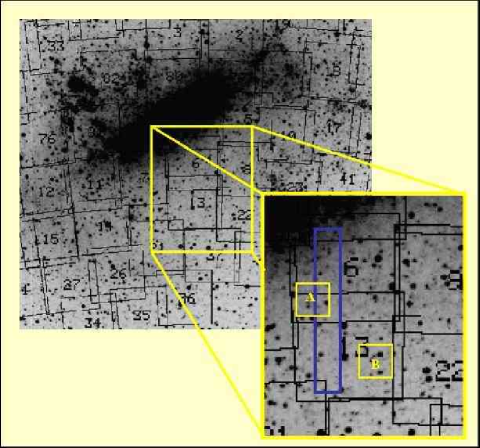
Figure 1: The light squares indicate the approximate positions of our observed fields with respect to MACHO’s fields # 6 and #13. The elongated rectangle identifies the position of the OGLE II field LMC_SC21.

The two positions were chosen in order to maximize the number of known RRd’s observable with only two pointings of the 1.54 m Danish telescope, since a major purpose of our study was to derive the mass-metallicity relation for double mode pulsators (Bragaglia et al. 2001). We expected to observe about 80 RR Lyrae’s according to A96 average density of RR Lyr’s in the LMC, among which 5 and 4 double mode RR Lyrae (RRd), in field A and B, respectively (Alcock et al. 1997, hereinafter A97). Coordinates (epoch 2000) of the two centers are: $\alpha$ = 5:22:48.49, $\delta$ = –70:34:06 (field A), and $\alpha$ = 5:17:35.7, $\delta$ = –71:00:13 (field B). In both observing runs the telescope was equipped with the DFOSC focal reducer. In 1999 data were acquired on a Loral/Lesser 2052x2052 pixel chip (CCD #C1W7, scale 0.4 arcsec/pix, field of view of 13.7 arcmin²), and a filter wheel mounting the Johnson standard system. Observations were done in the Johnson-Bessel $B$ and $V$ filters (ESO 450, and 451), and we obtained 58 $V$ and 27 $B$ frames for field A, and 55 $V$ and 24 $B$ frames for field B. Seeing conditions were quite variable during each night and the whole observing run; typical values were in the range 1.3-1.9 arcsec (see Table 1) .

Exposure times varied from 180 to 300 sec in $V$ and from 360 to 480 sec in $B$, depending on weather/seeing conditions and hour angle. They were chosen as an optimal compromise between S/N and time resolution of the light variations of the RR Lyrae variables. Eighteen stars from Landolt (1992) standard fields were observed during each night in order to secure the transformation to the standard Johnson photometric system.

In the 2001 run, data were acquired on an EEV 42-80 CCD (2048x4096 pixels, scale of 0.39 arcsec/pix and field of view of 13.7 arcmin²). The CCD has pixel size of 15 $\mu$m and is back-illuminated to increase its quantum efficiency, particularly at shorter wavelengths. Due to the field of view of the DFOSC focal reducer, only half of the CCD is actually used to image data. Observations were done in the Johnson-Bessel $B$, $V$ and in the $i$-Gunn filters (ESO 450, 451, and 425) and we obtained 14 $V$, 14 $B$ and 14 $i$ frames for field A, and 15 $V$, 14 $B$, and 14 $i$ frames for field B. Exposure times were of 360 sec in $B$, and 180 sec in $V$ and $i$.

Both nights of the 2001 run were fully photometric with good seeing conditions. Transparency and seeing were better in the second night with most frequent values of the seeing around 1.0 arcsec in $B$ and $V$, and 0.8 arcsec in $i$. A large number of standard stars in Landolt (1992) - Stetson (2000) standard fields PG0918+029, PG0231+051, PG1047+003, and SA98 were observed several times during both nights to estimate the nightly extinction and to tie the observations to the standard Johnson-Cousins photometric system (see Section 2.2). Two exposures of different length were taken at any pointings of the standard fields, in order to obtain well exposed measurements of both bright and faint standard stars.

2.1 Reductions

Reduction and analysis of the 1999 photometric data were done using the package DoPHOT (Schechter, Mateo & Saha 1993), which uses an elliptical Gaussian PSF to evaluate instrumental magnitudes. We used a PSF varying with the position on the frame and run DoPHOT independently on all frames, with a threshold for source detection of 5 $\sigma$ above the local sky. The resulting tables were then aligned to the “best” frame for each field (i.e., to the one taken in best seeing and weather conditions, and near meridian) and stars were counteridentified using a private software written by P. Montegriffo. Catalogues were produced, all containing the same number of stars, and with a unique identifying number: this helped in the following variability search and study. The number of objects classified as stars in each frame is variable (from several thousands to about 30,000). The final 1999 catalogues, after counteridentification in $V$ and $B$, contain about 29,000 objects for field A and about 23,000 for field B; this difference seems reasonable since field A is slightly closer to the LMC bar and thus more crowded than field B.

Photometric reductions of the 2001 data were done using DAOPHOT/ALLSTAR II (Stetson 1996) and ALLFRAME (Stetson 1994). DAOPHOT/ALLSTAR II allows to obtain very precise brightness estimates and astrometric positions for stellar objects in individual two-dimensional digital images starting from a rough initial estimate for the position and brightness of each star, and a model of the PSF for each frame. We used a source detection threshold of 4 $\sigma$ above the local sky background, and a PSF which varied quadratically with the position in the frame. Modelling of the PSF in each frame was obtained by considering a set of about 100 stars. The resulting PSFs are hybrid models consisting of an analytic function and a table of residuals, thus offering both the advantages of an analytic and of an empirical PSF.

Because of the high crowding of our LMC fields, in addition to DAOPHOT/ALLSTAR, reductions were executed with ALLFRAME, which performed the simultaneous consistent reductions of all the 2001 multicolour images of our fields: 42 frames for field A, and 43 frames for field B, respectively. By combining informations coming from all images it was thus possible to obtain a better precision in the identification and centering of the stars, and to resolve objects that appeared blended in frames with worse seeing conditions.

Aperture corrections were derived for the $B,\leavevmode\nobreak\ V,\leavevmode\nobreak\ I$ reference frames from about 10 bright and relatively isolated stars in each frame. The choice of these stars has been particularly difficult for field A, the more crowded one, for which we also derived larger corrections. The mean differences between PSF and aperture magnitudes were used to correct the PSF magnitudes of all other objects. The $B,\leavevmode\nobreak\ V,\leavevmode\nobreak\ I$ corrections (aperture minus PSF) were: –0.140, –0.073, –0.020 mag for field A, and –0.026, –0.035, –0.040 mag for field B respectively.

Aperture magnitudes for the photometric standard stars were computed using PHOT in DAOPHOT, rejecting all saturated stars and all objects with less than 1000 detected counts. The aperture radii for these stars were determined from curves of growth.

2.2 Night extinction calculation and absolute photometric calibration

Only the third night (January 6, 1999) of the 1999 run was fully photometric. Viceversa, both nights in the 2001 run were photometric and with good seeing conditions. Since the 2001 run was definitely superior both for photometric quality and seeing, and since a much larger number of standard stars were observed, our entire photometric data set has been tied to the standard Johnson-Cousins photometric system through the absolute photometric calibration of the 2001 run.

The extinction coefficients for the nights were computed from observations of the standard stars in the selected areas PG0918 and SA98 (Landolt 1992). We used 7 bright standard stars in PG0918, with measurements at different airmasses ($1.180<\sec z<1.626$) to estimate the extinction coefficients for the night of January 23, and 7 bright standard stars of SA98 with measurements at $1.145<\sec z<2.028$, to estimate the extinction for the night of January 24. The derived first order extinction coefficients are: $K_{V}=0.142\pm 0.008$, $K_{B}=0.240\pm 0.020$, and $K_{i}=0.071\pm 0.006$ for January 23; $K_{V}=0.123\pm 0.005$, $K_{B}=0.220\pm 0.009$, and $K_{i}=0.052\pm 0.010$ for January 24. These extinction coefficients well compare to the average ones for La Silla, as deduced from the relevant web pages.

Stetson (2000) has extended Landolt (1992) standard fields to a fainter magnitude limit, reaching $V\sim$ 20 mag. To transform to the standard Johnson-Cousins photometric system, we used Stetson (2000) standard star magnitudes, as available from the web site http://cadcwww.hia.nrc.ca/standards, for a large number of standards in Landolt’s fields PG0918+029, PG0231+051, PG1047+003, and SA98. We have verified that Stetson (2000) standard system reproduces very well the Johnson-Cousins standard system by Landolt (1992). In fact, if we restrict only to the original Landolt standards in each field, and derive the calibrating equations using both Landolt’s and Stetson’s values, the colour terms agree to the thousandth of magnitude both in $B$ and $V$. In $I$ there are two deviating stars, namely PG0231 for which Landolt’s $I$ magnitude is about 0.2 mag too bright, and SA98-1002 whose Landolt’s $I$ magnitude is about 0.02-0.04 mag fainter. If these two stars are discarded, agreement to within a thousandth of magnitude is found for the $I$ colour terms as well.

We measured magnitudes for 67 stars in these areas. However, since most of the new faint standard stars observed by Stetson (2000) only have $V$ measurements, while the $B$ and $I$ database is still poor, only a subset of 27 stars with accurate standard magnitudes in all three photometric pass-bands of our interest were actually used in the calibration procedure. Aperture photometry magnitudes of these stars measured in the two nights of the 2001 run, corrected for the extinction appropriate to each night, were combined to derive the following calibration equations:

$$B-b=0.111(\pm 0.032)\times(b-v)-5.472$$

$$V-v=0.021(\pm 0.017)\times(b-v)-5.175$$

$$I-i=-0.023(\pm 0.025)\times(v-i)-6.507$$

where $B,V,I$ are in the Johnson-Cousins system, while $b$, $v$, $i$ are the instrumental magnitudes. The calibration relations are are based on 127 measurements in the two nights of the 2001 run of the restricted sample of 27 standard stars with magnitude and colours in the ranges $12.773<V<17.729$, $-0.273<B-V<1.936$, $-0.304<V-I<2.142$. Note that we adopted an iterative rejecting procedure, eliminating those objects that deviated more than 2.5 $\sigma$ (where $\sigma$ is the standard deviation of the residuals) from the least square fit regression lines. Photometric zero points accuracies are of 0.02 mag in $V$ and 0.03 mag in $B$ and $I$, respectively.

2.3 Comparison between the 1999 and the 2001 photometries

Figure 2 shows the instrumental colour magnitude diagrams (CMDs) obtained from the photometric reductions of one $V$ and one $B$ frames of field A, from the 1999 and 2001 data sets respectively, using the various different packages employed in this study, namely DoPhot for the 1999 data set (left panel), DAOPHOT + ALLSTAR (central panel), and DAOPHOT + ALLSTAR + ALLFRAME (right panel) for the 2001 data set.

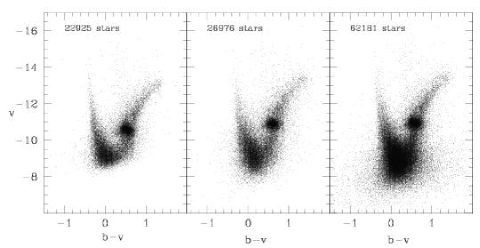
Figure 2: Comparison between instrumental CMDs (all based on two frames) of the 1999 and 2001 datasets. Left panel: DoPhot reductions of the 1999 data; central panel: DAOPHOT+ALLSTAR reductions of the 2001 data; right panel: DAOPHOT+ALLSTAR+ALLFRAME reductions of the 2001 data.

The figure very well illustrates the superiority of the 2001 data and reduction procedures with respect to the 1999 ones. In particular, the increased number of objects and the fainter magnitude limit reached by the 2001 data in the central panel of Figure 2 is due predominantly to the better seeing and photometric conditions and the improved sensitivity of the CCD in run 2001, and in part to the better performances of the DAOPHOT reduction package with respect to DoPhot. The CMD in the right panel demonstrates the efficiency and superiority of the ALLFRAME package to resolve and measure faint stellar objects in crowded fields: the number of stars in the right panel of the figure is more than doubled and reaches one magnitude fainter than data shown in the other two panels. For these reasons all considerations about the CMDs have been based on the ALLFRAME reductions of the 2001 data (see C03).

3 Identification of the variable stars

Variable stars were identified on the 1999 $v$ and $b$ instrumental time-series independently, using the program VARFIND, by P. Montegriffo. VARFIND performs the following actions: (i) normalizes the files containing measures of the fitted stars to a reference frame, using all stars in 1.5 magnitude bins about 2 magnitudes brighter than the expected average level of the RR Lyrae variables to determine mean frame-to-frame offsets with respect to the reference frames. As $v$ and $b$ reference frames we chose those taken in the best seeing and photometric conditions; (ii) computes the average magnitude of each star and its standard deviation by combining all frames in a given filter, using the offsets determined in step (i); (iii) displays the scatter diagrams of the average measurements, namely the standard deviations vs. average $<v>$ and $<b>$ plots from which candidate variables are identified thanks to their large rms and picked up interactively. In our scatter diagrams the RR Lyrae’s and the Cepheids define very well distinct groups of stars with large rms values, respectively at 18.6$<V<$19.8 mag and 15.1$<V<$16.6 mag; (iv) extracts the time-series sequence of each candidate variable and of its selected reference stars (see below).

The search procedure was repeated several times, subsequently lowering the detection threshold. Stars whose standard deviations of the $v$ and $b$ measurements were larger than 3 $\sigma$, where $\sigma$ is the rms of bona-fide non-variable stars at same magnitude level, were flagged as candidate variables and closely inspected for variability using the program GRATIS (GRaphycal Analyzer of TIme Series) a private software developed at the Bologna Observatory by P. Montegriffo, G. Clementini and L. Di Fabrizio. This code, directly interfaced to VARFIND, allows to display the sequence of differential measurements of the object with respect to the selected reference stable stars, as a function of the Heliocentric Julian day of observation, and to perform a period search on these data (see below). A total number of 1165 and 747 objects were checked for variability in fields A and B, respectively. We are confident that our identification of the RR Lyrae stars is rather complete, and we will come back to this point in Sections 3.2 and 5.

Variable stars were then counteridentified on the 2001 frames using private software by P. Montegriffo. A few further variables originally missed by the search on the 1999 data were recovered in the comparison with MACHO and OGLE II datasets (see Section 4). In the end the two fields were found to contain a total number of 162 short period variable stars (P$<$ 7 days), mainly of RR Lyrae type (125 single-mode and 10 double-mode, one of which not previously known from A97; see Section 5.1), and an additional 8 candidate variable objects: 5 possible binary systems, 1 possible ab-type RR Lyrae, and 2 other variables that we were not able to classify.

The number of variables divided by type and field is given in Table 2.

Table 2: Number and type of variables identified in the two fields

Type	Field A	Field B	Total
RRab	52	35	87
RRc	20	18	38
RRd	6	4	10
Anomalous Cepheid	3	1	4
Cepheids	10	1	11
Binaries	6	5	11
$\delta$ Scuti	1	—	1
Total	98	64	162
Candidate variables	5	3	8

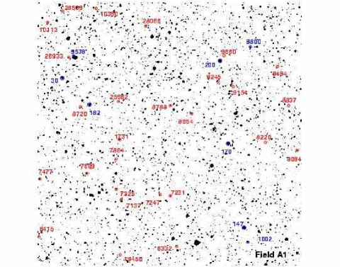
Figure 3: LMC sub-field A1 ($6.8^{\prime}\times 6.8^{\prime}$), North-East quadrant. North is up and East is left. Variables are marked by open circles. Identification numbers are as in Table 5.

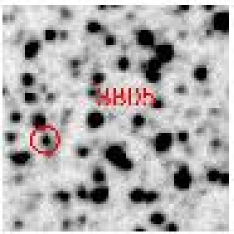
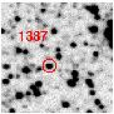
Figure 11: Left panel: finding chart of the ab-type RR Lyrae star # 3805, which is located slightly outside sub-field A4 in the East direction. Right panel: finding chart of the c-type RR Lyrae star # 1387, which is located slightly outside sub-field B4 in the South/East direction. Both maps show a 40 $\times$ 40 arcsec area, North is up and East is left.

Finding charts for all the variables are provided in Figures 3 to 10, where each field is divided in 4 quadrants 6.8${}^{\prime}\times 6.8^{\prime}$ large (subfields A1, A2, A3, A4, and B1, B2, B3, B4, respectively), which correspond to the pre-imaging fields of our spectroscopic study with FORS1 at the VLT (see G04). There is some overposition at the centre of the each set of 4 quadrants and a few objects appear twice. RR Lyrae stars are marked by red open circles in the electronic version of the finding charts, the other variables are in blue. Two RR Lyrae stars fall outside the FORS fields and are shown separately in Figure 11.

3.1 Period search and average quantities

All variables were studied using their differential photometry with respect to two stable, well isolated objects used as reference stars, whose constancy was carefully checked on the full 1999-2001 data set. Coordinates and calibrated magnitudes of the reference stars from the 2001 photometry are given in Table 3. Errors quoted in the table include both the internal error contribution given by ALLFRAME (about 0.005 mag in $V$ and $I$, and 0.004 mag in $B$), and the systematic errors in the transformation to the standard system (which include uncertainties of the aperture corrections: about 0.02 mag in $V$ and $I$ and 0.03 mag in $B$, and the zero points of the photometric calibration: $\pm 0.02$ mag in $V$, and $\pm 0.03$ mag in $B$ and $I$, see Section 2.2).

Note that in a preliminary analysis, variables were studied using their differential photometry with respect to a larger number of comparison stars selected in each field (namely four stars per field). However, since results were very much the same in the final study we used just one star per field, namely in each field the star with most accurate magnitude determinations and with colours better matching the RR Lyrae’s average colour. This procedure minimize any colour effect on the differential light curves and amplitudes of the variable stars, due to the colour of the comparison stars and the different colour response of the detectors used in the two runs.

Table 3: Coordinates and magnitudes of the comparison stars

Id	$\alpha_{2000}$	$\delta_{2000}$	$V$	nV	$B$	nB	$I$	nI
Field A
1253	5 22 57.93	$-$70 31 31.96	16.889$\pm$0.026	14	17.575$\pm 0.045$	14	16.102$\pm$0.025	14
Field B
128	5 16 29.75	$-$71 01 46.62	16.194$\pm$0.023	15	16.888$\pm 0.037$	14	15.410$\pm$0.035	14

In order to define the periodicities we run GRATIS on the instrumental differential photometry of the variable stars. GRATIS performs a period search according to two different algorithms: (a) the Lomb periodogram (Lomb 1976, Scargle 1982) and (b) the best-fit of the data with a truncated Fourier series (Barning 1962). We first performed the Lomb analysis on a wide period interval. Then the Fourier algorithm was used to refine the period definition and to find the best fitting model from which to measure the amplitude and average luminosity of each variable. The period search employed each of the complete (1999+2001) $\Delta b$, $\Delta v$, and $\Delta i$ data-sets. We derived periods and epochs accurate to the third-fourth decimal place for all the variable in our sample, well sampled the $B$ and $V$ light curves for about 95% of the RR Lyrae stars, and detected the Blazhko modulation of the light curve (Blazhko 1907) in about 17% of the RRab’s and 5.3% of the RRc’s (see Section 5). Complete coverage of the light variation was also obtained for 4 candidate Anomalous Cepheids (see Section 3.2), for 9 eclipsing binaries with short orbital period (P$<$1.4 days), and for 6 of the Cepheids. GRATIS also performs a search for multiple periodicities, and was run on the data of the 10 double-mode variables falling in our two fields, 9 in A97 and 1 newly discovered. However, our data sampling for these stars is inadequate to allow a very accurate derivation of the double-mode periodicities: on this particular aspect, the very extensive data set collected by MACHO and OGLE II are clearly superior to ours.

Best fitting models of the light variation were computed for all variables with full light curve coverage, using GRATIS. These models are based on Fourier series, with the number of harmonics generally varying from 1 to 5 for the c-type RR Lyrae’s, and from 4 to 12 for the ab-type variables. Intensity-average differential $<\Delta v>$, $<\Delta b>$, and $<\Delta i>$ magnitudes were derived for all the variables with complete light curves as the integral over the entire pulsation cycle of the models best fitting the observed data. By adding the instrumental magnitudes of the reference stars, we obtained the $b$, $v$, $i$ mean instrumental magnitudes of the variables, and the mean $B$, $V$, $I$ magnitudes in the Johnson-Cousins system were calculated using the calibration equations given in Section 2.2 and the aperture corrections in Section 2.1.

Average residuals from the best fitting models for RR Lyrae’s with well sampled light curves are 0.02-0.03 mag in $V$ and 0.03-0.04 mag in $B$ for the single-mode, non Blazhko variables, and 0.05-0.10 in $V$ and 0.06-0.12 in $B$ for the double-mode stars. The lower accuracy of the $B$ light curves is because the RR Lyrae stars are intrinsically fainter in this passband.

The individual $B,V,I$ photometric measurements of the variables are provided in Table 4. For each star we indicate the star identification number, the field where the star is located, the variable type, Heliocentric Julian Day of observations and corresponding $V$, $B$, $I$ magnitudes.

Table 4: $V,B,I$ photometry of the variable stars

Star #2525 - Field A - RRab
HJD	$V$	HJD	$B$	HJD	$I$
($-$2451183)		($-$2451183)		($-$2451933)
0.623172	19.708	0.626309	20.227	0.580303	18.666
0.630545	19.741	0.634897	20.243	0.608358	18.591
0.660672	19.738	0.666204	20.047	0.633786	18.731
0.670556	19.558	0.685707	19.517	0.683115	18.799
0.681100	19.231	0.704341	19.193	0.708370	18.712
0.690070	19.120	0.722720	19.010	0.757143	19.024
0.699977	19.006	0.747280	19.057	0.784249	19.127
0.708693	18.863	0.766320	19.206	1.574978	18.922
0.718368	18.831	0.785521	19.278	1.600522	18.922
0.727072	18.759	0.807245	19.430	1.625198	18.970

A portion of Table 4 is shown here for guidance regarding its form and content. The entire catalogue is available only electronically at CDS.

In Table 5 and 6 we summarize the main characteristics of the variables for stars in field A and B, separately. Namely we list: identifier, coordinates ($\alpha$ and $\delta$) at the 2000 equinox, variable star type, period, heliocentric Julian day (HJD) of maximum light for the pulsating variables (RR Lyrae’s, Cepheids and $\delta$ Scuti) and of the primary (deeper) minimum light for the eclipsing binaries, number of data-points on the $V,B,I$ light curves, $V,B,I$ mean magnitudes and amplitudes of the light curves, computed as the difference between maximum and minimum of the best fitting models, for the variable stars with complete coverage of the light variation. At the bottom of each table we also give informations on the candidate variables. The atlas of light curves is presented in the Appendix.

The average apparent luminosities of the RR Lyrae stars with full coverage of the light curve and without shifts between the 1999 and 2001 photometry are $<V>=19.417\pm 0.019$ ($\sigma$ =0.154, 67 stars), $<B>=19.816\pm 0.021$ ($\sigma$ =0.171, 67 stars) in field A, and $<V>=19.318\pm 0.022$ ($\sigma$ =0.157, 49 stars), $<B>=19.678\pm 0.023$ ($\sigma$ =0.159, 49 stars) in field B. These values (the $V$ average luminosities in particular) are fully consistent with those presented in C03. We refer to this paper for an in-depth discussion of their implications on the distance to the LMC and related issues. We also recall that our average luminosities for the field LMC RR Lyrae stars are in very good agreement with Walker (1992) mean apparent luminosity of the RR Lyrae stars in the LMC globular clusters (see Section 6 of C03).

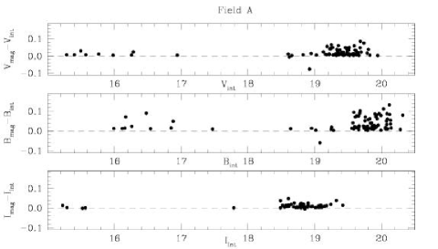
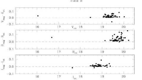
Figure 12: Differences between magnitude-averaged and intensity-averaged mean magnitudes for the variable stars in field A (upper panels) and B (lower panels), separately.

It has often been argued on the better way to compute the average magnitude of a variable star and on the colour that better represents the temperature of an RR Lyrae star (Sandage 1990, 1993; Carney, Storm & Jones 1992; Bono, Caputo & Stellingwerf 1995). The average magnitudes of the variable stars in Tables 5 and 6 were computed in two different ways, as intensity-averaged means (Columns 8,9,10) and as magnitude-averaged means (Columns 11,12,13). Based on theoretical grounds it has been claimed that large differences may exist between these two different types of averages, and that for RR Lyrae stars the difference may be as large as 0.1-0.2 mag in $V$ and $B$, respectively (Bono et al. 1995). In Figure 12 we plot the differences between the two types of averages for star in Field A and B separately. Magnitude-averaged mean magnitudes are generally fainter than the intensity-averaged mean magnitudes, and the differences increase for fainter magnitudes. However, they are generally small and only in a few cases exceed 0.1 mag. At the luminosity level of the RR Lyrae stars the average differences are $<V_{mag}-V_{int}>$=0.020, $<B_{mag}-B_{int}>$=0.035 and $<I_{mag}-I_{int}>$=0.010 for stars in Field A, and 0.022, 0.042, and 0.011 mag for stars in Field B.

Figures 13 and  14 show the position of the various types of variables in the $V,B-V$ CMDs of Field A and B.

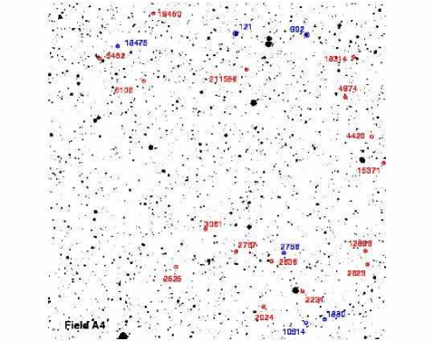
Figure 4: FORS1 LMC sub-field A4 ($6.8^{\prime}\times 6.8^{\prime}$), South-East quadrant. North is up and East is left. Variables are marked by open circles. Identification numbers are as in Table 5.

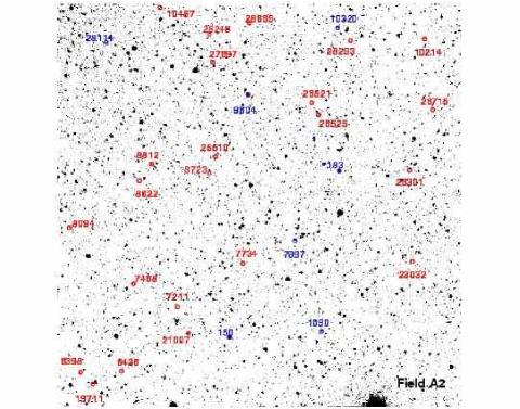
Figure 5: FORS1 LMC sub-field A2 ($6.8^{\prime}\times 6.8^{\prime}$), North-West quadrant. North is up and East is left. Variables are marked by open circles. Identification numbers are as in Table 5.

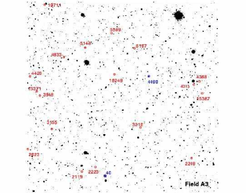
Figure 6: FORS1 LMC sub-field A3 ($6.8^{\prime}\times 6.8^{\prime}$), South-West quadrant. North is up and East is left. Variables are marked by open circles. Identification numbers are as in Table 5.

Figure 7: FORS1 LMC sub-field B1 ($6.8^{\prime}\times 6.8^{\prime}$), North-East quadrant. North is up and East is left. Variables are marked by open circles. Identification numbers are as in Table 6.

Figure 8: FORS1 LMC sub-field B4 ($6.8^{\prime}\times 6.8^{\prime}$), South-East quadrant. North is up and East is left. Variables are marked by open circles. Identification numbers are as in Table 6.

Figure 9: FORS1 LMC sub-field B2 ($6.8^{\prime}\times 6.8^{\prime}$), North-West quadrant. North is up and East is left. Variables are marked by open circles. Identification numbers are as in Table 6.

Figure 10: FORS1 LMC sub-field B3 ($6.8^{\prime}\times 6.8^{\prime}$), South-West quadrant. North is up and East is left. Variables are marked by open circles. Identification numbers are as in Table 6.

Table 5: Informations and average quantities for the variable stars in field A.

Id	$\alpha$	$\delta$	Type	P	Epoch	Np	$<{\rm V_{int}}>$	$<{\rm B_{int}}>$	$<{\rm I_{int}}>$	$<{\rm V_{mag}}>$	$<{\rm B_{mag}}>$	$<{\rm I_{mag}}>$	AV	AB	AI	Notes
	(2000)	(2000)		(days)	($-$2400000)	(V,B,I)	(mag)	(mag)	(mag)	(mag)	(mag)	(mag)	(mag)	(mag)	(mag)
1731	5:23:38.69	-70:31:08.17	ab	0.58245	51183.63490	6,14,$-$	$-$	$-$	$-$	$-$	$-$	$-$	$-$	1.100:	$-$	Incomplete
2525	5:23:32.39	-70:39:15.34	ab	0.61615	51933.57692	69,41,$-$	19.340	19.764	$-$	19.376	19.826	$-$	0.991	1.272	$-$
2767	5:23:17.70	-70:38:55.90	ab	0.53106	51183.52271	64,33,$-$	19.467	19.874	19.074	19.517	19.962	19.089	1.091	1.363	$-$
3061	5:23:25.13	-70:38:28.94	ab	0.47622	51182.69038	66,41,11	19.631	20.037	19.220	19.679	20.121	19.239	0.809	1.093	0.765	Blazhko
3805	5:24:04.69	-70:37:18.42	ab	0.62740	51185.78000	60,37,10	19.402	19.866	18.850	19.415	19.889	18.848	0.623	0.805	0.345
3948	5:22:40.34	-70:37:16.96	ab	0.66656	51182.61069	69,40,14	19.292	19.686	18.628	19.331	19.757	18.647	0.959	1.287	0.654	Blazhko?,(a)
4313	5:21:33.88	-70:36:52.65	ab	0.64222	51933.55000	54,33,9	19.270	19.779	18.451	19.276	19.791	18.488	0.356	0.454	$-$
4933	5:22:29.99	-70:35:53.61	ab	0.61350	51182.85143	65,32,13	19.103	19.531	18.542	19.127	19.572	18.546	0.793	1.044	0.442	Blazhko?
4974	5:22:51.21	-70:35:47.69	ab	0.58069	51933.57692	69,41,11	19.384	19.809	18.778	19.406	19.850	18.801	0.764	1.039	0.482
5106	5:22:14.40	-70:37:43.54	ab	0.56476	51183.84000	46,29,12	18.820	18.939	18.587	18.827	18.952	18.596	0.391:	0.565:	0.455::	Blend
5148	5:22:20.87	-70:35:34.08	ab	0.56862	51186.68716	71,39,12	$-$	$-$	$-$	$-$	$-$	$-$	$-$	$-$	$-$	(b)
5167	5:21:59.65	-70:35:34.99	ab	0.63023	51934.57159	64,33,11	19.359	19.837	18.808	19.373	19.864	18.822	0.570	0.765	0.550:
5331	5:23:15.30	-70:35:14.46	ab	0.58234	51185.61000	32,21,14	19.673	20.079	19.103	19.696	20.133	19.107	0.932:::	1.192	0.322
5452	5:23:51.03	-70:35:01.06	ab	0.67849	51933.62602	67,38,12	19.296	19.799	$-$	19.309	19.812	$-$	0.589	0.569	$-$
5589	5:22:09.54	-70:35:02.50	ab	0.63648	51934.60800	59,33,11	19.574	20.079	18.942	19.578	20.089	18.949	0.364	0.417	0.391:	Blazhko?
6398	5:22:40.71	-70:33:50.18	ab	0.56026	51182.78609	70,41,12	19.317	19.745	18.730	19.347	19.802	18.736	0.883	1.156	0.561
6426	5:22:32.47	-70:33:48.73	ab	0.66224	51182.78094	70,41,14	19.185	19.584	18.555	19.227	19.660	18.569	1.045	1.312	0.707
7211	5:22:21.12	-70:32:43.96	ab	0.51978	51182.97180	67,36,14	$-$	$-$	$-$	$-$	$-$	$-$	0.875::	1.377::	0.655:::	Incomplete
7247	5:23:25.53	-70:32:33.45	ab	0.56171	51182.56088	70,40,14	19.408	19.795	18.857	19.429	19.835	18.852	0.714	0.865	0.422
7325	5:23:39.08	-70:32:24.81	ab	0.48677	51183.68571	68,40,13	19.435	19.845	18.893	19.479	19.927	18.906	1.131	1.449	0.677
7468	5:22:30.00	-70:32:20.56	ab	0.63550	51182.79217	62,37,12	19.615	20.126	18.850	19.622	20.142	18.855	0.492	0.692	0.304:
7477	5:24:02.92	-70:32:08.60	ab	0.65641	51183.08070	69,40,14	19.183	19.552	18.670	19.249	19.628	18.695	1.108	1.371	0.730
7609	5:23:48.34	-70:32:00.33	ab	0.57336	51182.80975	65,38,14	19.313	19.699	$-$	19.340	19.751	$-$	0.788	1.004	$-$
7734	5:22:07.82	-70:31:59.83	ab	0.61699	51183.25568	53,24,$-$	$-$	$-$	$-$	$-$	$-$	$-$	0.502	0.661	$-$	(c)
						13,14,10	$-$	$-$	$-$	$-$	$-$	$-$	0.519	0.673	0.311
8094	5:22:43.00	-70:31:23.70	ab	0.74575	51182.23076	60,40,13	19.353	19.891	18.676	19.360	19.908	18.682	0.452	0.644	0.323
8220	5:22:52.79	-70:31:11.11	ab	0.67684	51182.92564	70,41,12	19.469	19.920	18.770	19.483	19.949	18.780	0.608	0.829	0.382
8720	5:23:50.14	-70:30:16.73	ab	0.65767	51934.68800	66,38,14	19.129	19.489	18.590	19.185	19.584	18.607	1.163	1.447	0.760
8788	5:23:22.35	-70:30:14.64	ab	0.55960	51183.01548	70,41,14	19.444	19.844	$-$	19.482	19.916	$-$	0.939	1.240	0.830:::	Blazhko
9154	5:23:02.88	-70:29:44.63	ab	0.61981	51933.61768	67,40,11	19.552	20.032	18.931	19.569	20.059	18.933	0.662	0.755	0.255	Blazhko,(d)
						53,26,$-$	$-$	$-$	$-$	$-$	$-$	$-$	0.759	0.913	$-$
						14,14,11	$-$	$-$	$-$	$-$	$-$	$-$	0.384	0.478	0.263::
9245	5:23:07.61	-70:29:36.50	ab	0.55980	51182.81277	65,38,12	$-$	$-$	$-$	$-$	$-$	$-$	0.706	0.948	0.402::	(e)
9494	5:22:49.20	-70:29:13.50	ab	0.57860	51185.74736	69,40,12	19.217	19.584	$-$	19.266	19.674	$-$	1.150	1.410	$-$
9660	5:23:05.71	-70:28:56.83	ab	0.62181	51183.68200	67,41,14	19.392	19.862	18.795	19.407	19.890	18.796	0.669	0.811	0.312
10214	5:21:31.10	-70:28:12.01	ab	0.59994	51934.74600	60,32,10	19.204	19.639	$-$	19.217	19.665	$-$	0.633	0.824	$-$
10487	5:22:24.55	-70:27:40.52	ab	0.58957	51182.40810	54,38,12	19.569	20.022	18.886	19.603	20.073	18.896	0.913	1.106	0.603
12896	5:22:46.09	-70:38:54.95	ab	0.57368	51185.65865	71,37,12	19.589	20.027	18.955	19.620	20.087	18.964	0.911	1.248	0.691
15371	5:22:41.56	-70:37:07.14	ab	0.58712	51185.66370	31,28,12	19.460	19.874	18.557	19.480	19.936	18.605	0.929	1.201	0.957
15387	5:21:30.38	-70:37:11.30	ab	0.55983	51933.58300	58,30,5	19.612	20.043	$-$	19.630	20.075	$-$	0.705	0.839:	$-$
16249	5:22:08.22	-70:36:31.00	ab	0.60475	51183.72300	71,41,13	19.378	19.759	18.844	19.430	19.837	18.847	1.118	1.403	0.360	Blazhko,(d)
						57,27,$-$	$-$	$-$	$-$	$-$	$-$	$-$	1.252	1.500	$-$
						14,14,13	$-$	$-$	$-$	$-$	$-$	$-$	0.764	1.090	0.337:
18314	5:22:49.08	-70:34:59.12	ab	0.58711	51183.17420	70,41,13	19.410	19.790	18.815	19.459	19.793	18.835	1.120	1.426	0.719
19450	5:23:37.89	-70:34:06.71	ab	0.39792	51182.55700	70,41,14	19.662	19.983	19.286	19.737	20.116	19.324	1.344	1.709	1.098
19711	5:22:38.14	-70:34:02.02	ab	0.55296	51181.77241	29,18,14	19.200	19.535	18.607	19.244	19.606	18.617	0.961	1.148	0.756
21007	5:22:18.85	-70:33:10.84	ab	0.75730	51933.80000	14,13,8	19.319	19.841	18.487	19.323	19.851	18.488	0.340	0.456	0.162
25301	5:21:33.95	-70:30:24.47	ab	0.56059	51182.71139	63,32,12	19.766	20.237	$-$	19.805	20.317	$-$	1.005	1.359	$-$
25362	5:23:38.48	-70:30:08.55	ab	0.57746	51182.73348	70,41,14	19.443	19.816	18.764	19.488	19.903	18.785	1.078	1.466	0.671::
25510	5:22:13.37	-70:30:11.50	ab	0.64956	51183.78150	64,38,11	19.150	19.614	18.554	19.160	19.631	18.561	0.609	0.707	0.417	Blazhko?
26525	5:21:52.45	-70:29:28.68	ab	0.52288	51186.67057	66,37,14	19.473	19.913	$-$	19.507	19.991	$-$	0.863	1.269	$-$
26821	5:21:53.90	-70:29:17.47	ab	0.58755	51185.75937	65,39,13	19.624	20.097	19.097	19.644	20.132	19.104	0.752	0.989	0.473
26933	5:23:53.78	-70:28:59.71	ab	0.48829	51186.66446	59,35,14	19.295	19.577	18.750	19.355	19.679	18.754	1.188	1.490	0.791
28066	5:23:30.05	-70:28:11.07	ab	0.59975	51933.60857	51,24,$-$	$-$	$-$	$-$	$-$	$-$	$-$	0.496	0.666	$-$	(f)
						13,14,12	$-$	$-$	$-$	$-$	$-$	$-$	0.503	0.629	0.326
28246	5:22:14.65	-70:28:06.71	ab	0.47777	51934.62544	15,32,10	19.605	20.030	19.144	19.660	20.106	19.182	1.270	1.543	1.023
28293	5:21:46.08	-70:28:13.20	ab	0.66148	51186.76300	56,24,7	19.520	20.053	$-$	19.524	20.062	$-$	0.403	0.553	0.472:::	(g)
28539	5:23:55.73	-70:27:48.61	ab	0.61388	51934.75195	68,36,11	19.533	19.916	18.796	19.592	20.028	18.815	1.149	1.495	0.707
2024	5:23:10.96	-70:40:03.33	c	0.36008	51933.70166	72,40, 8	19.500	19.876	19.165	19.513	19.893	19.177	0.509	0.606	0.455
2119	5:22:22.20	-70:39:59.98	c	0.26526	51934.60511	64,39,10	19.659	19.986	19.407	19.663	19.990	19.421	0.297	0.354	0.479::::
2223	5:22:16.48	-70:39:50.18	c	0.28784	51934.58000	67,36,10	19.556	19.836	19.136	19.568	19.856	19.145	0.493	0.604	0.499
2234	5:23:01.41	-70:39:44.47	c	0.32280	51933.74938	38,26,$-$	$-$	$-$	$-$	$-$	$-$	$-$	0.531	0.664	$-$	(f)
						14,14,12	$-$	$-$	$-$	$-$	$-$	$-$	0.425	0.584	0.389
2623	5:22:45.59	-70:39:11.37	c	0.29130	51183.62631	65,40,13	19.368	19.631	19.046	19.379	19.649	19.057	0.441	0.595	0.454
2636	5:23:09.26	-70:39:08.61	c	0.31611	51934.76812	69,40,7	19.595	19.896	19.080	19.605	19.919	19.083	0.464	0.633	0.234
3216	5:21:57.05	-70:38:25.85	c	0.21824	51185.76536	67,39,$-$	$-$	$-$	$-$	$-$	$-$	$-$	0.407	0.515	$-$	(h)
						53,26,$-$	$-$	$-$	$-$	$-$	$-$	$-$	0.411	0.526	$-$
						14,13,14	$-$	$-$	$-$	$-$	$-$	$-$	0.392	0.513	0.405
4388	5:21:31.63	-70:36:46.15	c	0.34194	51185.64493	63,30, 9	19.427	19.758	$-$	19.431	19.764	$-$	0.305	0.363	0.200::
6332	5:23:20.39	-70:33:53.53	c	0.25047	51933.59613	68,41,14	19.433	19.753	19.005	19.439	19.766	19.007	0.374	0.527	0.300	Blazhko,(i)
				0.24961	51933.57400	14,14,14	19.444	19.750	19.023	19.452	19.764	19.027	0.383	0.531	0.298

Table 5: - continued -

Id	$\alpha$	$\delta$	Type	P	Epoch	Np	$<{\rm V_{int}}>$	$<{\rm B_{int}}>$	$<{\rm I_{int}}>$	$<{\rm V_{mag}}>$	$<{\rm B_{mag}}>$	$<{\rm I_{mag}}>$	AV	AB	AI	Notes
	(2000)	(2000)		(days)	($-$2400000)	(V,B,I)	(mag)	(mag)	(mag)	(mag)	(mag)	(mag)	(mag)	(mag)	(mag)
6415	5:24:03.13	-70:33:38.44	c	0.44299	51186.74600	64,38,12	19.206	19.573	18.713	19.215	19.583	18.715	0.438	0.473	0.229
7231	5:23:22.37	-70:32:35.39	c	0.32349	51183.11007	66,36,14	19.322	19.643	18.861	19.331	19.664	18.866	0.413	0.607	0.287
7864	5:23:39.20	-70:31:38.15	c	0.31347	51182.78235	67,39,14	19.464	19.774	19.047	19.475	19.792	19.050	0.433	0.545	0.233
8622	5:22:28.87	-70:30:35.86	c	0.32082	51934.69553	66,39,14	19.542	19.868	19.103	19.552	19.887	19.108	0.429	0.628	0.307
8812	5:22:26.38	-70:30:19.05	c	0.35485	51182.82224	69,41,14	19.397	19.767	18.821	19.410	19.791	18.829	0.515	0.626	0.396
8837	5:22:45.64	-70:30:14.33	c	0.31629	51182.66999	64,41,14	19.566	19.905	19.057	19.580	19.927	19.061	0.501	0.631	0.328
10113	5:24:00.31	-70:28:06.22	c	0.35231	51186.78595	69,40,14	19.486	19.878	18.891	19.494	19.894	18.895	0.415	0.535	0.321
10360	5:23:45.34	-70:27:44.11	c	0.27926	51934.58000	53,26,$-$	$-$	$-$	$-$	$-$	$-$	$-$	0.431	0.541	$-$	(f)
						13,13,13	$-$	$-$	19.199	$-$	$-$	19.201	0.363	0.507	0.203
26715	5:21:29.21	-70:29:23.32	c	0.35646	51182.69358	52,25,$-$	19.378	19.725	$-$	19.388	19.746	$-$	0.486	0.678	$-$	(l)
27697	5:22:13.98	-70:28:34.98	c	0.38293	51184.64328	66,39,$-$	19.166	19.541	18.744	19.174	19.554	18.746	0.396	0.471	$-$	Blazhko?,(m)
						53,25,$-$	$-$	$-$	$-$	$-$	$-$	$-$	0.380	0.486	$-$
						13,14,11	$-$	$-$	$-$	$-$	$-$	$-$	0.485	0.513	0.229:
28665	5:22:06.49	-70:27:55.55	c	0.30047	51183.77067	64,38,$-$	$-$	$-$	$-$	$-$	$-$	$-$	0.348	0.536	$-$	(n)
						52,25,$-$	$-$	$-$	$-$	$-$	$-$	$-$	0.336	0.553	$-$
						12,13,12	$-$	$-$	19.264	$-$	$-$	19.270	0.422	0.564	0.342
2249	5:21:33.31	-70:39:51.28	d	0.30731	51182.99235	70,41,12	19.372	19.704	18.878	19.389	19.729	18.903	0.600	0.709	0.744::
3155	5:22:35.25	-70:38:28.39	d	0.38161	51934.66700	66,40,14	19.209	19.577	18.792	19.218	19.598	18.803	0.419	0.664	0.496
				0.38141
4420	5:22:44.66	-70:36:35.68	d	0.35989	51182.65973	72,41,14	19.409	19.726	18.784	19.417	19.740	18.794	0.419	0.554	0.432
7137	5:23:37.64	-70:32:41.42	d	0.34301	51934.60052	72,40,14	19.413	19.736	$-$	19.420	19.750	$-$	0.413	0.557	0.424
8654	5:23:15.72	-70:30:27.24	d	0.34544	51183.77084	66,35,12	19.269	19.651	18.848	19.275	19.658	18.849	0.475	0.817	0.113
23032	5:21:33.40	-70:31:57.24	d	0.34226	51182.93313	71,39,13	19.597	19.993	$-$	19.682	20.081	$-$	0.693	0.935	$-$
28114	5:22:35.51	-70:28:15.66	$\delta$S	0.11268	51183.63220	69,40,11	19.940	20.273	$-$	19.943	20.280	$-$	0.280	0.388	0.185
9578	5:23:52.36	-70:28:57.87	AC	0.54758	51186.81780	62,34,12	18.626	19.277	17.789	18.620	19.293	17.790	0.307	0.576	0.205
9604	5:22:07.01	-70:29:07.41	AC	0.61569	51182.38306	62,29,12	18.932	19.234	18.550	18.947	19.253	18.558	0.655	0.774	0.532
10320	5:21:48.72	-70:28:00.82	AC	0.29177	51185.76536	66,37,14	18.655	19.236	$-$	18.658	19.244	$-$	0.264	0.419	$-$
30	5:23:55.92	-70:29:31.92	Ceph.	3.66050	51933.77646	67,41,14	15.396	15.980	$-$	15.403	15.992	$-$	0.392	0.532	$-$
40	5:22:12.23	-70:40:09.81	Ceph.	2.39797	51934.66602	69,40,13	15.753	16.237	15.212	15.765	16.260	15.225	0.501	0.691	0.513
121	5:23:17.88	-70:34:30.81	Ceph.	2.13218	51180.99088	66,41,12	15.975	16.532	15.288	15.980	16.543	15.290	0.344	0.472	0.205::
147	5:22:59.43	-70:33:24.15	Ceph.	4.69248	51181.61046	67,37,14	15.467	16.099	$-$	15.497	16.170	$-$	0.830	1.218	$-$
150	5:22:10.50	-70:33:14.98	Ceph.	3.13782	51181.70621	56,36,14	16.251	16.837	15.524	16.257	16.852	15.523	0.415	0.574	$-$
170	5:23:04.43	-70:31:13.83	Ceph.	6.66000	51933.30000	64,35,12	15.277	16.105	$-$	15.284	16.117	$-$	0.394	0.568	$-$
182	5:23:47.50	-70:30:13.46	Ceph.	2.80545	51184.80502	61,38,14	15.820	16.389	$-$	15.862	16.479	$-$	0.940	1.354	$-$
183	5:21:48.21	-70:30:25.86	Ceph.	2.49288	51182.99807	68,39,10	16.259	16.830	15.566	16.283	16.879	15.567	0.689	0.976	0.193:::
200	5:23:07.02	-70:29:05.06	Ceph.	2.73228	51179.44316	61,41,14	15.568	16.142	14.920	15.575	16.156	14.921	0.424:	0.571	0.208
902	5:23:00.61	-70:34:32.31	Ceph.	1.17104	51182.99969	69,41,13	16.936	17.460	$-$	16.941	17.469	$-$	0.368	0.487	$-$
1880	5:22:56.07	-70:40:17.73	EB	2.18677	51183.76190	69,40,13	18.997	19.139	$-$	18.921	19.078	$-$	$-$	$-$	$-$
2756	5:23:06.01	-70:38:57.82	EB	1.18211	51183.81265	70,39,14	19.327	19.595	$-$	19.342	19.612	$-$	0.733	0.781	$-$
4490	5:21:53.47	-70:36:35.13	EB	1.38051	51184.69877	70,39,10	19.016	19.011	19.017	19.022	19.015	19.020	0.727	0.523	$-$
9800	5:22:57.60	-70:28:43.46	EB	0.59749	51184.78793	66,41,14	18.590	18.627	18.504	18.602	18.638	18.518	0.617	0.626	0.592
10914	5:23:00.60	-70:40:22.44	EB	0.56184	51183.79300	65,39,13	19.767	20.041	$-$	19.784	20.058	$-$	0.689	0.647	0.615::
18475	5:23:46.56	-70:34:46.31	EB	0.80928	51185.66801	60,41,12	19.821	19.872	$-$	19.826	19.880	$-$	0.452	0.570	$-$
1002	5:22:58.16	-70:33:46.41	EB	$-$	$-$	$-$	$-$	$-$	$-$	$-$	$-$	$-$	$\sim$0.29	$\sim$0.32	$>$0.2
1090	5:21:51.82	-70:33:08.41	EB	$-$	$-$	$-$	$-$	$-$	$-$	$-$	$-$	$-$	$\sim$0.23	$\sim$0.34	$>$0.3
3276	5:24:04.96	-70:38:06.35	?	$-$	$-$	70,38,14	19.040	19.268	18.862	19.051	19.279	18.877	$>$0.5	$>$0.6	$>$0.6
7997	5:21:57.21	-70:31:36.27	EB?	$-$	$-$	$-$	$-$	$-$	$-$	$-$	$-$	$-$	$\sim$0.14	$\sim$0.46	$>$0.5
8723	5:22:14.60	-70:30:27.49	EB	$\sim$1.16	51183.78600	51,21,14	19.152	19.859	$-$	19.161	19.862	18.455	0.789	$-$	$-$

Notes:
(a) The minimum light in 2001 is systematically brighter than in 1999 both in $B$ and $V$, possibly indicating a Blazhko modulation.

(b) No reliable average magnitudes and amplitudes are available since in 1999 the star occasionally fell on a CCD bad column.

(c) The 2001 light curves are systematically fainter than the 1999 ones. The star could be an unresolved blend in the 1999 photometry. Amplitudes and average luminosities are provided for the 1999 (upper line) and 2001 data (lower line), separately.

(d) Amplitudes and average luminosities are provided for the combined 1999 + 2001 data (upper line), and for the 1999 (middle line) and 2001 data (lower line), separately.

(e) The 2001 light curves are systematically fainter than the 1999 ones. The star could either be an unresolved blend in the 1999 photometry, or could be affected by Blazhko effect. Amplitudes correspond to the 1999 data-set.

(f) The 2001 light curves are systematically brighter than the 1999 ones. Amplitudes and average luminosities are provided for the 1999 (upper line) and 2001 data (lower line), separately.

(g) Light curves are very noisy possibly indicating the presence of secondary periodicities.

(h) The 2001 light curves are systematically slightly brighter than in 1999, particularly in $B$. Amplitudes are provided for the combined 1999 + 2001 data (upper line), and for the 1999 (middle line) and the 2001 data (lower line), separately.

(i) Period and shape of the 2001 light curves are slightly different than in 1999. Amplitudes and average luminosities are provided for the combined 1999+2001 data (upper line) and for the 2001 data (lower line), separately.

(l) The star was not observed in 2001. (m) Amplitudes and average luminosities are provided separately for the combined 1999 + 2001 data (upper line), for the 1999 data (middle line), and for the 2001 data (lower line). (n) The 2001 light curves are systematically fainter than the 1999 ones. Amplitudes are provided separately for the combined 1999 + 2001 data (upper line), for the 1999 data (middle line), and for the 2001 data (lower line).

Table 6: Informations and average quantities for the variable stars in field B.

Id	$\alpha$	$\delta$	Type	P	Epoch	Np	$<{\rm V_{int}}>$	$<{\rm B_{int}}>$	$<{\rm I_{int}}>$	$<{\rm V_{mag}}>$	$<{\rm B_{mag}}>$	$<{\rm I_{mag}}>$	AV	AB	AI	Notes
	(2000)	(2000)		(days)	($-$2400000)	(V,B,I)	(mag)	(mag)	(mag)	(mag)	(mag)	(mag)	(mag)	(mag)	(mag)
1408	5:17:13.79	-71:06:06.91	ab	0.62600	51182.73500	52,31,14	19.343	19.772	18.777	19.369	19.813	18.778	0.812	0.978	0.376:
1575	5:16:31.27	-71:05:48.49	ab	0.67389	51182.40483	70,37,14	19.250	19.666	18.690	19.290	19.733	18.703	1.029	1.284	0.740
1907	5:18:12.30	-71:04:59.49	ab	0.58048	51182.92634	55,23,$-$	$-$	$-$	$-$	$-$	$-$	$-$	0.658	0.796	$-$	Blazhko,(a)
						70,37,13	19.287	19.724	18.726	19.306	19.762	18.739	$-$	$-$	$-$
2055	5:17:17.39	-71:04:50.18	ab	0.52295	51182.41018	47,34,12	$-$	$-$	$-$	$-$	$-$	$-$	0.749:::	1.304	0.534::
2249	5:17:13.01	-71:04:27.10	ab	0.61044	51933.59040	69,35,14	19.346	19.775	18.689	19.371	19.823	18.728	0.747	0.987	0.634
2379	5:18:43.16	-71:04:03.24	ab	0.48854	51182.14762	66,36,13	$-$	$-$	$-$	$-$	$-$	$-$	0.931::	1.292::	0.482::::	Incomplete
2407	5:16:51.61	-71:04:13.40	ab	0.67004	51182.54647	68,36,14	19.186	19.613	18.531	19.201	19.639	18.539	0.652	0.818	0.466	Blazhko?
2884	5:16:52.13	-71:03:25.18	ab	0.61943	51183.71406	70,36,11	19.217	19.630	18.655	19.249	19.689	18.639	0.869	1.182	0.475::
3033	5:18:13.98	-71:03:00.56	ab	0.49938	51933.59874	69,37,14	$-$	$-$	$-$	$-$	$-$	$-$	1.157:	1.254:	0.371::::	Incomplete
3054	5:17:45.36	-71:03:01.45	ab	0.50798	51183.21819	68,35,14	19.066	19.440	$-$	19.089	19.486	$-$	0.902	1.149	$-$
3400	5:17:14.46	-71:02:26.58	ab	0.48616	51182.21055	67,37,14	19.469	19.805	18.824	19.530	19.921	18.851	1.263	1.619	0.836
3412	5:18:38.21	-71:02:14.47	ab	0.53020	51182.91258	68,36,13	19.425	19.834	18.856	19.460	19.902	18.876	0.834	1.159	0.707
4244	5:16:27.60	-71:00:59.85	ab	0.55621	51182.84333	70,37,14	19.260	19.633	18.782	19.297	19.702	18.808	0.944	1.159	$-$	Blazhko?,(b)
						55,23,$-$	$-$	$-$	$-$	$-$	$-$	$-$	0.881	1.179	$-$
						15,14,14	$-$	$-$	$-$	$-$	$-$	$-$	1.122	1.399	0.800
4540	5:16:13.67	-71:00:28.34	ab	0.56892	51182.52598	61,31, 8	19.414	19.801	18.858	19.450	19.866	18.878	0.880	1.208	0.668	(c)
4780	5:16:53.00	-71:00:02.53	ab	0.61757	51934.63778	69,35,14	19.396	19.860	18.707	19.411	19.895	18.718	0.595	0.972	$-$	Blazhko?,(b)
						54,21,$-$	$-$	$-$	$-$	$-$	$-$	$-$	0.592	0.930	$-$
						15,14,14	$-$	$-$	$-$	$-$	$-$	$-$	0.466::::	0.673:::	0.499
4859	5:16:10.87	-70:59:54.34	ab	0.52336	51184.68400	46,21,$-$	19.240	19.617	$-$	19.294	19.687	$-$	1.061	1.182	$-$	(c)
5394	5:17:15.73	-71:04:11.37	ab	0.50993	51182.86900	64,31,11	19.463:	19.957:	19.117:	19.499:	19.976:	19.121:	$>$0.643	$>$0.735	0.318	Incomplete
5902	5:16:12.23	-70:58:04.86	ab	0.56975	51182.87903	54,23,$-$	19.121	19.472	$-$	19.165	19.571	$-$	1.015	1.282	$-$	(c)
5950	5:18:06.56	-70:57:48.52	ab	0.49957	51182.07579	55,24,14	$-$	$-$	$-$	$-$	$-$	$-$	$>$0.4	$>$0.5	$-$	Incomplete
6020	5:16:32.44	-70:57:53.68	ab	0.61428	51183.70139	53,22,$-$	$-$	$-$	$-$	$-$	$-$	$-$	0.858	0.973	$-$	(d)
						15,14,14	$-$	$-$	$-$	$-$	$-$	$-$	0.931	1.157	0.534
6440	5:16:16.68	-70:57:11.56	ab	0.49482	51934.75800	43,23,13	19.247	19.612	18.865	19.280	19.664	18.876	0.875	1.053	0.592
6798	5:17:11.33	-70:56:32.65	ab	0.58405	51182.44080	53,22,$-$	19.253	19.658	18.711	19.291	19.730	18.720	1.035	1.376	$-$	Blazhko,(e)
						15,14,14	$-$	$-$	$-$	$-$	$-$	$-$	0.760	1.043	0.499
7063	5:18:43.98	-70:55:55.77	ab	0.65428	51183.79572	68,36,13	19.195	19.629	18.549	19.213	19.654	18.569	0.633	0.686	0.457	Blazhko?
7158	5:16:45.89	-71:03:27.94	ab	0.80192	51182.91400	54,28,12	19.198	19.610	18.452	19.212	19.636	18.462	0.679	0.830	0.433
7442	5:17:15.68	-70:55:26.77	ab	0.57795	51933.63581	70,36,14	19.426	19.835	18.855	19.446	19.876	18.877	0.650	0.917	0.655
7620	5:18:03.53	-70:55:03.12	ab	0.65616	51182.75690	70,37,14	19.079	19.409	18.461	19.133	19.489	18.471	1.071	1.366	0.710
7652	5:17:32.87	-71:03:13.94	ab	0.50700	51934.78000	61,36,12	19.426	19.763	19.191	19.492	19.888	19.207	1.270	1.629	0.811
10692	5:18:04.54	-71:04:34.91	ab	0.55094	51182.70020	68,37,14	19.548	19.956	18.918	19.574	20.009	18.938	0.862	1.109	0.747:	Blazhko?
10811	5:18:15.95	-71:04:27.07	ab	0.47637	51182.81620	69,36,14	19.431	19.797	$-$	19.492	19.893	$-$	1.166	1.392	0.452
14449	5:17:05.32	-71:01:40.85	ab	0.58413	51934.57998	64,36,13	19.514	19.851	18.727	19.450	19.906	18.734	0.804	1.016	0.329::
19037	5:16:20.66	-70:58:06.31	ab	0.41128	51933.76200	67,33,14	19.702	20.023	19.293	19.784	20.174	19.332	1.466	1.821	0.917
21801	5:16:36.29	-70:58:21.72	ab	0.50723	51182.88136	68,34,14	19.598	20.013	19.216	19.627	20.067	19.235	0.874	1.198	0.653::
22917	5:18:19.05	-70:54:56.03	ab	0.56468	51182.63629	60,35,14	19.426	19.797	18.887	19.462	19.863	18.893	0.957	1.283	0.729
23502	5:18:01.58	-70:54:31.81	ab	0.47217	51934.61759	46,31,9	19.385	19.662	$-$	19.446	19.792	$-$	1.296	1.638	1.300:::	(c)
24089	5:17:44.64	-70:54:03.08	ab	0.55977	51183.74000	55,21,$-$	19.365	19.798	$-$	19.370	19.797	$-$	0.371	0.485	1.386	(f)
						$-$,14,8	$-$	$-$	$-$	$-$	$-$	$-$	1.339	$-$	$-$
1387	5:18:47.52	-71:05:58.35	c	0.36448	51185.77393	69,36,14	19.252	19.561	18.737	19.263	19.580	18.741	0.443	0.587	0.316
2517	5:16:31.25	-71:04:03.32	c	0.23176	51934.70774	69,36,12	19.695	19.925	19.374	19.706	19.943	19.379	0.452	0.555	0.312
2811	5:18:31.15	-71:03:21.74	c	0.27757	51183.04260	70,35,13	19.384	19.691	18.956	19.389	19.699	18.958	0.313	0.371	0.242
3625	5:16:52.66	-71:02:01.87	c	0.27654	51182.93263	61,35,14	$-$	$-$	$-$	$-$	$-$	$-$	0.292	0.379	$-$	(g)
						46,21,$-$	$-$	$-$	$-$	$-$	$-$	$-$	0.305	0.343	$-$
						15,14,14	$-$	$-$	$-$	$-$	$-$	$-$	0.322	0.378	0.194
				0.27995	51182.89758	59,35,$-$	$-$	$-$	$-$	$-$	$-$	$-$	0.297	0.403	$-$
						44,21,$-$	$-$	$-$	$-$	$-$	$-$	$-$	0.293	0.360	$-$
						15,14,14	$-$	$-$	$-$	$-$	$-$	$-$	0.308	0.379	0.197
3957	5:18:39.60	-71:01:12.61	c	0.34232	51182.70003	68,35,13	19.533	19.932	19.038	19.543	19.948	19.050	0.427	0.509	0.218
4008	5:17:04.72	-71:01:17.28	c	0.28474	51934.75471	66,34,14	19.281	19.559	18.855	19.290	19.574	18.859	0.421	0.507	0.282
4179	5:17:19.90	-71:01:02.08	c	0.35587	51186.69270	50,29,14	19.173	19.502	18.640	19.183	19.520	18.644	0.438	0.560	0.298
4749	5:17:49.67	-71:00:01.38	c	0.32703	51184.82256	63,35,13	19.314	19.653	18.834	19.321	19.667	18.838	0.394	0.512	0.306
4946	5:18:11.02	-70:59:35.60	c	0.31275	51934.63003	68,34,12	19.432	19.739	18.929	19.443	19.757	18.933	0.433	0.561	0.298
5256	5:18:45.57	-70:58:56.79	c	0.34248	51182.67690	70,36,14	19.259	19.614	18.795	19.268	19.628	18.796	0.417	0.527	0.210
6164	5:18:10.12	-70:57:30.75	c	0.37487	51934.68304	70,36,14	19.057	19.353	18.604	19.068	19.374	18.613	0.451	0.615	0.389
6255	5:17:17.83	-70:57:26.43	c	0.35239	51933.61784	58,33,11	19.264	19.600	18.807	19.272	19.614	18.810	0.380	0.539	0.223
6957	5:18:18.03	-70:56:08.75	c	0.40567	51182.81240	70,37,13	19.197	19.532	18.673	19.205	19.549	18.680	0.396	0.568	0.370
7064	5:18:18.59	-70:55:58.64	c	0.40070	51934.75034	70,37,13	19.122	19.433	18.644	19.135	19.454	18.655	0.474	0.607	0.451
7490	5:18:44.67	-70:55:10.81	c	0.30481	51186.72128	70,37,13	$-$	$-$	$-$	$-$	$-$	$-$	0.505	0.637	$-$	(h)
						55,22,$-$	$-$	$-$	$-$	$-$	$-$	$-$	0.483	0.528	$-$
						15,14,13	$-$	$-$	$-$	$-$	$-$	$-$	0.568	0.709	0.430
7648	5:16:38.53	-70:55:09.52	c	0.34268	51186.66994	69,35,14	19.384	19.688	18.947	19.399	19.707	18.951	0.467	0.598	0.339
7783	5:17:25.70	-70:54:51.95	c	0.34634	51933.69588	70,35,12	19.279	19.564	18.828	19.298	19.596	18.837	0.553	0.742	0.417
10585	5:17:29.07	-71:04:45.16	c	0.26954	51934.63450	70,37,12	19.628	19.934	19.158	19.641	19.959	19.167	0.478	0.657	0.407:

Table 6: - continued -

Id	$\alpha$	$\delta$	Type	P	Epoch	Np	$<{\rm V_{int}}>$	$<{\rm B_{int}}>$	$<{\rm I_{int}}>$	$<{\rm V_{mag}}>$	$<{\rm B_{mag}}>$	$<{\rm I_{mag}}>$	AV	AB	AI	Notes
	(2000)	(2000)		(days)	($-$2400000)	(V,B,I)	(mag)	(mag)	(mag)	(mag)	(mag)	(mag)	(mag)	(mag)	(mag)
3347	5:16:26.98	-71:02:36.58	d	0.36040	51182.84429	70,37,14	19.204	19.547	18.762	19.211	19.558	18.765	0.372	0.452	0.256
4509	5:17:36.92	-71:00:28.22	d	0.37130	51934.77500	69,37,14	19.462	19.823	18.717	19.468	19.833	18.725	0.333	0.429	0.397
6470	5:16:45.06	-70:57:07.67	d	0.36979	51934.63003	70,37,14	19.207	19.571	18.831	19.218	19.583	18.840	0.448	0.480	0.258
7467	5:18:17.14	-70:55:16.22	d	0.35775	51183.81805	70,37,14	19.043	19.372	18.597	19.055	19.389	18.599	0.487	0.560	0.252
5952	5:18:04.30	-70:57:50.13	AC	0.63300	51183.69855	64,35,12	18.459	19.120	17.648	18.463	19.135	17.631	0.325	0.601	0.274
204	5:17:54.15	-70:55:16.84	Ceph.	3.11055	51182.93750	68,36,13	16.009	16.620	$-$	16.038	16.679	$-$	0.765:	1.058:	$-$
1710	5:18:13.72	-71:05:19.83	EB	0.73439	51186.68150	70,34,14	19.402	19.501	19.240	19.416	19.518	19.232	0.643	0.650	0.682
5357	5:16:32.35	-70:59:00.82	EB	1.02684	51183.35399	70,37,14	19.288:	19.424:	$-$	19.066:	19.226:	$-$	1.015:::	1.039:::	$-$
6499	5:17:48.42	-70:56:57.99	EB	0.60784	51184.77200	68,34,14	19.376	19.500	$-$	19.383	19.509	$-$	0.401	0.433	0.329
15500	5:17:15.83	-71:00:50.06	EB	0.78568	51184.71789	66,37,14	19.792	19.884	$-$	19.805	19.899	$-$	0.620	0.704	$-$
21007	5:18:21.08	-70:56:27.16	EB	1.35753	51186.69270	68,34,14	20.010	20.207	$-$	20.024	20.226	$-$	0.639	0.790	0.503
2601	5:18:39.98	-71:03:41.03	EB	$-$	$-$	$-$	$-$	$-$	$-$	$-$	$-$	$-$	$\sim$0.61	$\sim$0.63	$>$0.3
3969	5:17:45.59	-71:01:17.38	?	9.90::	$-$	$-$	$-$	$-$	$-$	$-$	$-$	$-$	$\sim$0.21	$\sim$0.23	$>$0.15
7699	5:17:03.10	-70:55:00.65	RR?	$-$	$-$	14,5,$-$	$-$	$-$	$-$	$-$	$-$	$-$	0.600:	0.500:	$-$

Notes:

(a) Amplitudes are from the 1999 data set (upper line), average luminosities are from the combined 1999+2001 data set (lower line).

(b) Amplitudes and average luminosities are provided separately for the combined 1999 + 2001 data (upper line), for the 1999 data (middle line), and for the 2001 data (lower line).

(c) The star was not observed in 2001.

(d) The 2001 light curves are systematically fainter than the 1999 ones. Amplitudes and average luminosities are provided for the 1999 (upper line) and 2001 data (lower line), separately.

(e) Amplitudes and average luminosities are provided for the 1999 (upper line) and 2001 data (lower line), separately.

(f) The star does not have $V$ observations in 2001. The 1999 $B$ light curve has a different shape and amplitude than the 2001 one. Amplitudes and average luminosities for the 1999 data are provided in the fist line, the $B$ amplitude of the 2001 data in the second line.

(g) The 2001 light curves are systematically brighter and have smaller amplitudes than the 1999 ones. Both in 1999 and 2001 the V data provide a slightly different period than the B ones. Amplitudes and average luminosities are provided separately for the combined 1999 + 2001 data (upper line), for the 1999 data (middle line), and for the 2001 data (lower line), and for each of the two periodicities.

(h) The 2001 light curves are systematically fainter than the 1999 ones. Amplitudes are provided for the combined 1999 + 2001 data (upper line), for the 1999 data (middle line), and for the 2001 data (lower line), separately.

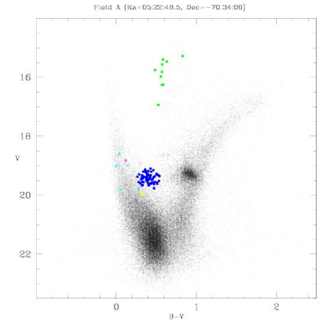
Figure 13: Position of the variable stars on the $V$ vs $B-V$ colour - magnitude diagram of field A. Different symbols are used for the various type of variables (RR Lyrae stars: filled circles; candidate Anomalous Cepheids: open squares; blended variables: asterisks; Cepheids: filled squares; binaries: filled triangles; crosses: $\delta$ Scuti) which are plotted according to their intensity average magnitudes and colours.

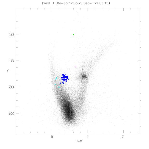
Figure 14: Same as Figure 13 for the variable stars in Field B.

Variable stars are plotted according to their intensity-averaged magnitudes and colours, and with different symbols corresponding to different types. $B,V,I$ magnitudes and coordinates (in pixels) of all the stars shown in these figures (63409 in field A and 58556 in field B) are available in electronic form at CDS.

3.2 The variable stars just above the horizontal branch

Our sample contains 5 variables (star #5106, #9578, #9604 and #10320 in Field A, and star #5952 in field B) with periods in the range from 0.29 to 0.63 days, which is typical of RR Lyrae stars, but with $V$ average magnitudes from 0.5 to about 0.9 mag brighter than the average luminosities of the RR Lyrae in the same fields (see open squares and asterisk in Figures 13 and 14). They also have amplitudes generally smaller than the RR Lyrae of similar period. Average luminosities and amplitudes of these stars are summarized in Table 7 where, in columns 7 and 8, we also list the difference in magnitude with respect to the average luminosity of the RR Lyrae stars in the same field (see Section 3.1).

Table 7: Characteristcs of the 5 variables above the HB

Id	Field	$<V>$	$<B>$	AV	AB	$\Delta V$	$\Delta B$	$<SHARP_{V}>$	$<SHARP_{B}>$
5106	A	18.820	18.939	0.391	0.565	0.597	0.877	+0.286	+0.337
9578	A	18.626	19.277	0.307	0.576	0.787	0.535	+0.264	+0.220
9604	A	18.932	19.234	0.655	0.774	0.481	0.578	+0.099	+0.110
10320	A	18.655	19.236	0.264	0.419	0.758	0.576	$-$0.209	$-$0.340
5952	B	18.459	19.120	0.325	0.601	0.862	0.560	+0.144	+0.092

Notes: $\Delta V$=$<V_{RR}>-<V_{*}>$, $\Delta B$=$<B_{RR}>-<B_{*}>$

These objects could be RR Lyrae variables blended with stars of comparable luminosity on the red and blue sides of the horizontal branch (HB) of the old stellar population in the LMC, namely clump and/or young main sequence stars. Indeed, star # 5952 in field B is considered the blend of an RR Lyrae and a red giant in MACHO web catalogue of variable stars (Alcock et al. 2003a, see Section 4.2.1). Table 8 shows schematically how the luminosities and amplitudes of a typical RR Lyrae in field A (namely the ab-type RR Lyrae # 2525) are expected to change, during the pulsation cycle, were the star blended to a red giant with luminosity equal to the average magnitude of the clump stars in the same field: $<V_{Clump\leavevmode\nobreak\ A}>$=19.304, and $<B_{Clump\leavevmode\nobreak\ A}>$=20.215 mag, according to C03. The comparison between light curves of resolved and blended variable is shown in Figure 15.

Table 8: Blend of an ab-type RR Lyrae and a clump star in field A

$<V_{RR}>$=19.326   $<B_{RR}>$=19.757
AV(RR)=0.882   AB(RR)=1.177
$<V_{Clump\leavevmode\nobreak\ A}>$=19.304   $<B_{Clump\leavevmode\nobreak\ A}>$=20.215
Phase	$V_{RR}$	$B_{RR}$		$V_{RR+Clump}$	$B_{RR+Clump}$
0.00	18.798	19.026		18.269	18.713
0.10	19.024	19.331		18.402	18.933
0.20	19.191	19.625		18.493	19.128
0.30	19.318	19.819		18.558	19.246
0.40	19.477	20.019		18.634	19.360
0.50	19.542	20.012		18.664	19.356
0.60	19.583	20.114		18.682	19.411
0.70	19.580	20.156		18.681	19.433
0.80	19.680	20.203		18.723	19.456
0.90	19.592	19.994		18.686	19.346
1.00	18.798	19.026		18.269	18.713
$<V_{RR+Clump}>$=18.551   $<B_{RR+Clump}>$=19.190
AV(RR+Clump)=0.454   AB(RR+Clump)=0.743
$\Delta V$=$<V_{RR+Clump}>-<V_{RR}>$ = 0.775
$\Delta B$=$<B_{RR+Clump}>-<B_{RR}>$ = 0.567

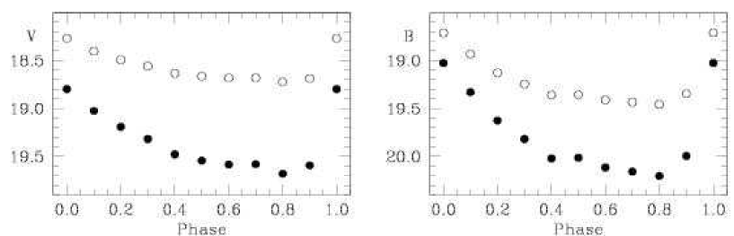
Figure 15: Schematic light curves of a resolved ab-type RR Lyrae star in field A (filled circles) and of its blend with a clump star in the same field (open circles).

This exercise shows that as the result of the blend the variable star would appear about 0.8 and 0.6 mag brighter than its average $V$ and $B$ luminosities of RR Lyrae star, its $V$ amplitude would be reduced by about 50% and the $B$ amplitude by about 37%. These numbers are very similar to the $\Delta V$ and $\Delta B$ value and amplitudes listed in Table 7, thus showing that blending is a plausible cause of the overluminosities of these 5 variable stars. In order to further investigate the blending hypothesis we checked the frames. Stars # 9578 and #9604 appear to be rather isolated. Stars # 10320, #5952 and #5106 instead have faint companions that may occasionally fall within the PSF of the primary star in bad seeing conditions. This should produce an increased scatter of the light curves as is indeed the case for star # 5106 which also is rather blue ($B-V$=0.119) indicating that this RR Lyrae is likely blended with a main sequence star. The other 4 objects in Table 7 have instead all rather clean light curves (star # 5952 in particular) and show no shifts between the 1999 and 2001 light curves that might hint they could be unresolved blends in our 1999 photometry, which was taken in less favourable seeing conditions.

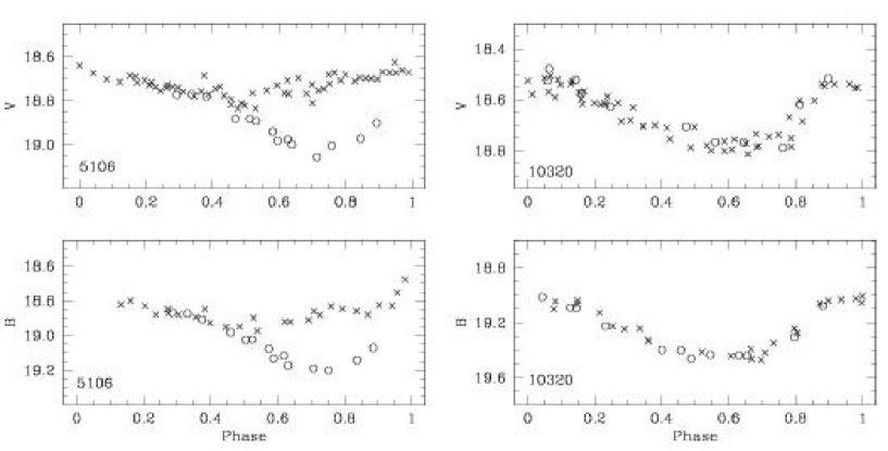
Figure 16: Light curves of the variable stars # 5106 (left panels) and # 10320 (right panels), open circles and crosses correspond to the 2001 and 1999 data, respectively.

Figure 16 shows the B,V light curves of star # 5106 (left panels) and # 10320 (right panels). The 1999 light curves of # 5106 are overluminous, particularly at minimum light, and have smaller amplitudes compared to the 2001 ones, as if the star was an unresolved blend in the 1999 photometry, those of star # 10320 do not show any systematic difference between the two datasets.

For each photometrized object DAOPHOT returns a shape defining parameter called SHARP, which is related to the intrinsic angular size of the object image and measures the regularity and symmetry of the PSF stellar profile. According to DAOPHOT user manual objects with values of $SHARP>>$ 0 are galaxies and blended doubles, objects with values of $SHARP<<$ 0 are cosmic rays and image defects. In our 2001 photometry stars at the luminosity level of the HB generally have: $\mid SHARP\mid<$ 0.10$-$0.20. Average $SHARP$ values for the 5 overluminous variables are given in Columns 9 and 10 of Table 7. Stars # 5952 and # 9604 have very good $SHARP$ values, $SHARP$ of star # 9578 is worse but still acceptable. Star # 10320 has negative values of $SHARP$ reflecting the fact that is at the frame edge where there are geometric distorsions. Finally, # 5106 has large positive values of $SHARP$ possibly indicating that the star is double. In conclusion, star # 5106 is likely a blended variable, while if the other four stars are actually blends, the two components must be completely unresolved, so to appear as just one single object within the PSF profile.

Tests with artificial stars performed to evaluate the completness of our photometry in field A show that at the luminosity level of the RR Lyrae and clump stars (19.20 $\leq V\leq$ 19.40 mag) our photometry is complete to 96.5 %. Since there are 78 RR Lyrae stars in field A we thus estimate that about 2-3 of this type of variables may be lost due to incompletness/blending, and, roughly scaling down to the smaller number of RR Lyrae stars and lower crowding, less than 2 in field B. These estimates are reasonably consistent with the number of variables detected just above the HB in each field.

G04 obtained spectra with FORS1 at the Very Large Telescope (VLT) and measured the metallicity of 3 of the overluminous variables. All of them appear as single objects in the FORS1 slit. The derived metallicities are: [Fe/H]=$-1.96\pm 0.16$ for #9604, [Fe/H]=$-1.66\pm 0.09$ for #10320, and [Fe/H]=$-1.59\pm 0.03$ for #5952, for an average value of [Fe/H]=$-1.74\pm 0.11$. The spectra of these 3 objects are shown in figures 9 and 21 of G04, along with those of LMC RR Lyrae and clump stars, and of Anomalous Cepheids (ACs) in $\omega$ Cen (see G04 figure 20), taken with the same instrumental set-up. The 3 stars have spectra very similar to the ACs in $\omega$ Cen. No clear evidence of spectral features due to secondary unresolved componens are seen, however star # 5952 has a prominent G-band similar to that observed in the spectrum of the clump star shown in figure 9 of G04.

The 5 overluminous variables were observed by MACHO and classified respectively as: ab-type RR Lyrae stars (# 5106 and # 9604), an RRab blended with a red giant (# 5952), and eclipsing binaries (# 9578 and 10320; see Table 9). The average $V$ magnitudes of stars # 5106 and 5952 agree with ours within 0.05 mag, with our values being systematically fainter. Stars # 10320, # 9604 and 9578 are instead brighter in our photometry, by 0.14, 0.17 and 0.27 mag, respectively. Nevertheless, even in MACHO photometry they lie above the HB.

Finally, we note that stars # 9604 and # 10320 were also observed by OGLE II (see Section 4.3 and Table 14) and classified ab- and c-type RR Lyrae, respectively. OGLE II average luminosities and light curves of star # 9604 agree within 0.1 mag, with our values being slightly brighter (by 0.04 mag in $B$ and 0.11 mag in $I$, see Table 14). Similarly, OGLE II $B$ data for star # 10320 agree within 0.03 mag to our value, being 0.03 mag fainter (we do not have $I$ photometry for this star). However, OGLE II $V$ average luminosities are respectively 0.79 and 0.71 mag fainter than ours, causing these two variables to have rather unlikely colours for RR Lyrae stars: ($B-V$)₉₆₀₄=$-$0.45, ($V-I$)₉₆₀₄=1.21 mag, and ($B-V$)₁₀₃₂₀=$-$0.17, ($V-I$)₁₀₃₂₀=1.53 mag in OGLE II photometry. Indeed, the OGLE II $V$ light curves of these objects are very poor. No actual $V$ light variation is seen for # 10320, possibly indicating a mismatched $B,V,I$ counteridentification.

In conclusion, based on the available observational evidences star # 5106 is likely to be the blend of an ab-type RR Lyrae with a young main sequence star. Instead, it is not possible to definitely assign a classification to the other 4 overluminous variables. Sub-arcsec photometry would be needed to shed some light on this issue.

On the other hand, given the complex stellar population in the LMC, we should also consider whether these 4 objects could be pulsating variables intrinsically brighter that the RR Lyrae stars, such as the Anomalous Cepheids (ACs) commonly found in dwarf Spheroidal galaxies (Pritzl et al. 2002 and references therein), or the low luminosity (LL) Cepheids (Clementini et al. 2003b) and the short period Classical Cepheids (SPCs) found in a number of dwarf Irregular galaxies (Smith et al. 1992, Gallart et al. 1999, 2004, Dolphin et al. 2002).

Anomalous Cepheids are metal-poor (Population II) helium burning stars in the instability strip, from about 0.5 up to about 2 mag (Bono et al. 1997) brighter than the HB of the old stars. They generally have periods in the range 0.3-2 days, but are too luminous for their periods to be Population II Cepheids (Wallerstein & Cox 1984). The high luminosity can be accounted for if they are more massive than normal old HB stars, as if they formed from the coalescence of a close binary (originally a blue straggler), although in some cases they may result from the evolution of younger, single massive stars. At low metallicities (Z$\leq$0.0004, i.e. [Fe/H]$\leq-1.7$), a hook in the HB is predicted, the so called “HB turnover” (see Caputo 1998, and references therein), so that stars with masses larger than $\sim 1.3M_{\odot}$ may cross the instability strip. Thus, there is a limiting metallicity above which no Anomalous Cepheid should be generated (Bono et al. 1997, Marconi et al. 2004). This limit in metallicity should be about [Fe/H]$\sim-1.7$ for variables around $\sim 1.3M_{\odot}$ and [Fe/H]$\sim-2.3$ for variables around $\sim 1.8M_{\odot}$. While very common in dwarf Spheroidal galaxies, Anomalous Cepheids are very rare in globular clusters: only one is known in the very metal-poor cluster NGC 5466 (Zinn & Dahn 1976, [Fe/H]=$-2.22$ according to Harris 1996) and two suspected ones are found in $\omega$ Cen (Nemec et al. 1994, Kaluzny et al. 1997), a cluster spanning a wide range in metallicity (Norris, Freeman, & Mighell 1996, Suntzeff & Kraft 1996, Pancino et al. 2002) and suspected of being the remnant of a disrupted dwarf galaxy.

The short period Cepheids are blue loop stars, i.e. stars that have ignited the helium in non degenerate cores ($M\geq 2.5M_{\odot}$), and have periods shorter than 10 days. They fall on the extension to short periods of the Classical Cepheids P/L relations (see Smith et al. 1992, Gallart et al. 1999, 2004, Dolphin et al. 2002).

Observed for the first time in NGC 6822 dwarf Irregular galaxy (Clementini et al 2003b), the LL Cepheids have small amplitudes, luminosities just above the HB, and are fainter and have shorter periods than the short period Cepheids.

It is not possible to decide to which of the above classes these four variables brighter than the HB more likely belong, based on the period-luminosity (P/L) relations, since at their short periods the P/L relations of Anomalous and Classical Cepheids merge and are almost indistinguishable. Indeed, in the P/L plane stars #9604, #5952 and #9578 fall on the extension to short periods of the fundamental mode Anomalous and Classical Cepheids, while star #10320 lies on the extension to short periods of the first overtone P/L relations (see Figure 2 of Baldacci et al. 2004). Knowledge of the metallicity may allow to break the degeneracy in the P/L relation, since short period Classical Cepheids and ACs are expected to have different metallicities, similar to those of their respective Population I and II parent populations. Based on the individual and average metallicities G04 conclude that the three overluminous variables they analyzed would more likely be ACs with masses $M\sim 1.3M_{\odot}$ rather than the short period tail of the LMC Classical Cepheids. Star #9578 lacks a metallicity estimate, hence its possible classification as AC is more uncertain.

4 A star by star comparison with MACHO and OGLE II photometries

4.1 Introduction

Fields A and B are contained in MACHO’s fields #6 and #13, respectively, and there is a 42.1% overlap between field A and OGLE II field LMC_SC21. Both MACHO and OGLE II catalogues are available on line. In particular, the MACHO collaboration has made available on web (see http://wwwmacho.mcmaster.ca/Data/MachoData.html) coordinates and instrumental photometry for about 9 milion LMC stars, and instrumental time-series for all the variables they have identified in the LMC. For the variables they also publish calibrated average magnitudes. Calibrated photometric maps (including time-series data of the variable stars) for all the LMC fields observed by OGLE II are instead available on OGLE II web page at http://www.astrouw.edu.pl/$\sim$ogle/ogle2/rrlyr_lmc.html. It was thus possible to make a detailed comparison between our and MACHO and OGLE II photometries, for both variables and constant stars in common.

Before going into the details of this comparison we note that two major differences exist between our, MACHO, and OGLE II databases: (i) observing strategy, exposures and time resolution of our photometric observations were specifically designed to achieve a very accurate definition of the average luminosity level of the RR Lyrae stars in the bar of the LMC, and provide a valuable counterpart to Walker (1992) study of the RR Lyrae stars in the LMC globular clusters. RR Lyrae’s are instead by-products close to the limiting magnitude of MACHO and OGLE surveys, whose main target was the detection of microlensing events in the LMC; (ii) although we used DoPhot to reduce the 1999 time series, the final photometry and calibration of our full dataset was handled by DAOPHOT+ALLFRAME, while both MACHO and OGLE II photometries used the DoPhot package. These packages may give similar results when crowding is not too severe; however DAOPHOT+ALLFRAME is much more efficient than DoPhot to resolve and measure faint stellar objects in crowded fields. This is clearly shown in Figure 2, where, thanks to ALLFRAME, we reach about 1-1.5 mag fainter and resolve almost twice the number of stars as with DoPhot. Moreover, DoPhot is reported to give systematically brighter magnitudes for faint stars in crowded regions than DAOPHOT due to its sky fitting procedure (Alcock et al. 1999, hereinafter A99). These differences should be kept in mind to interpret the results of the comparisons discussed in the next subsections.

4.2 Comparison with MACHO photometry

The MACHO collaboration has published calibrated photometry, namely magnitude-averaged mean magnitudes (Alcock et al. 2003a), only for the LMC variable stars. A99 provide a detailed description of the photometric calibration to the Kron-Cousins $V$ and $R$ system of the twenty top-priority MACHO fields of the LMC which include fields #6 and #13. They quote an internal precision of $\sigma_{V}$=0.021 mag (based on 20,000 stars with $V\;\lower 2.58334pt\hbox{$\sim$}\kern-7.75pt\raise 2.79857pt\hbox{$<$}\;$ 18 mag) and, from the comparison with other published measurements, they estimate a mean offset between MACHO and all the other data of $\Delta V$=$-$0.035 mag (see fig. 7 of their paper). A99 calibration is referred to as version 9903018 in following publications of the MACHO team (e.g. Alcock et al. 2004). However, the calibrated average magnitudes available on MACHO web pages (which, at the time this paper is being written, correspond to the last update of April 18th 2002) are based on a different version of A99 photometric calibration (see Alcock et al. 2004). MACHO catalogue is undoubtedly an invaluable inventory of the LMC variable star content; however, because of the non-standard passbands, the severe “blending” problems in the fields close to the LMC bar, and the complexity of the calibration procedures (see A99 for details), the absolute photometric calibration is a major concern. As a matter of fact different versions of the MACHO calibrated light curves exist, and it would be very important to know which version most closely matches the standard system in order to be able to fully exploit the catalogue. While working at the present paper we discussed this issue with members of the MACHO team who were working on the calibration procedures and/or were using the MACHO variable star catalogues (namely Dr.s D. Alves, C. Clement, and G. Kovács). We exchanged datasets and made comparisons between our photometry and data based on different versions of the MACHO photometric calibrations. In the following we report results based on 4 different datasets of MACHO’s photometry, namely:

1. MACHO’s magnitude-averaged mean values for the variables in common (77 and 54 variables in field A and B, respectively) as published on MACHO web pages. This comparison is described in Section 4.2.1.

2. MACHO’s time-series photometry for 42 RR Lyrae stars (25 in Field A and and 17 in field B, respectively), kindly made available by G. Kovács. This point-to-point comparison of the light curves is described in Section 4.2.2.

3. MACHO’s magnitude-averaged mean magnitudes for 7 c-type RR Lyrae stars (3 in Field A and and 4 in field B, respectively) whose data were sent us by C. Clement (see Section 4.2.3).

4. MACHO’s photometry for 18 RR Lyrae stars (9 in each field) and for the non-variable stars in 4${}^{\prime}\times 4^{\prime}$ areas surrounding the variables, whose photometric data were kindly made available by D. Alves. These comparisons are described in Sections 4.2.4 and 4.2.5, respectively.

4.2.1 Comparison with MACHO photometry for the variable stars in common: the web catalogue

We have retrieved from the MACHO web archive coordinates and magnitude-averaged mean magnitudes for all the variables identified by MACHO in our fields A and B and counteridentified the variable stars in common by coordinates using private software by P. Montegriffo. Counteridentifications between our and MACHO identification numbers are provided in Table 9 where we also give the classifications.

Table 9: Counteridentification between MACHO and us for the variable stars in common in field A and B, separately

Field A
IdMACHO	Id${}_{this\leavevmode\nobreak\ paper}$	TypeMACHO	Type${}_{this\leavevmode\nobreak\ paper}$
6.7055.7	30	Ceph.1st	Ceph
6.6810.11	40	Ceph.1st	Ceph
6.6931.37	57	EB	?
6.6932.22	121	Ceph.1st	Ceph
6.6933.19	147	Cep.Fun	Ceph
6.6812.27	150	Cep.Fun	Ceph
6.6933.11	170	Cep.Fun	Ceph
6.7054.10	182	Cep.Fun	Ceph
6.6934.10	200	EB	Ceph
6.6810.79	242	EB	?

Table 9 is presented in its entirety in the electronic edition of the Journal. A portion is shown here for guidance regarding its form and content.

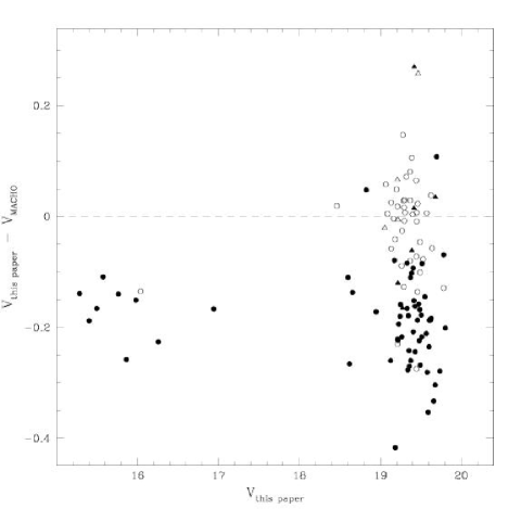
Figure 17: Comparison between our and MACHO mean $V$ magnitudes for the variable stars in common. Residuals are: this paper $-$ MACHO. Filled and open symbols are used for variable stars in field A and B, respectively. Triangles are the double mode RR Lyrae stars.

MACHO detected 85 variables in the portion of their field # 6 in common with our field A. We have counteridentified all of them. Three of these stars (MACHO numbers: 6.6810.67, 6. 7052.518, and 6.7054.463, corresponding to our stars: # 354, 3394 and 17341) are not found to significantly vary in our photometry. Other 5 variables classified eclipsing binaries by MACHO, some of which with very long period (P$>$ 60 day), have small amplitudes, sometime rather dubious in our photometry. On the other hand, we have identified 26 additional variables apparently missed by MACHO; they include 18 RR Lyraes (10 RRab’s and 8 RRc’s), 5 eclipsing binaries, 1 Cepheid, 1 $\delta$ Scuti, and 1 candidate variable of unknown type. Thus we have about 34% more short period variables than MACHO in field A.

57 variables have been found by MACHO in the area in common with field B. We have counteridentified 56 of them. The missing object is at the very edge of our field B and its photometry is not reliable. Two of the variables in common, classified by MACHO as eclipsing binaries, have rather small and dubious amplitudes in both photometries. In field B we have identified 13 additional variables that were not detected by MACHO; they include 9 RR Lyraes (3 RRab’s and 6 RRc’s) and 4 eclipsing binaries. Thus we have about 24% more short period variables than MACHO in field B.

We also noticed that MACHO classification of some of the variable stars in common does not match ours (see Columns 3 and 4 of Table 9). In particular, there are 6 variables classified as eclipsing binaries by MACHO that we classify as RR Lyrae stars (3) and Cepheids (1 Classical and 2 candidate ACs), 2 RR Lyrae for MACHO that we classify as an eclipsing binary and the blend of an RRab and a main sequence star, and an RR Lyrae + giant branch star for MACHO that we classify as candidate Anomalous Cepheid. Finally we assign a different pulsation mode to 13 other variables, classified as RR Lyrae stars in both photometries.

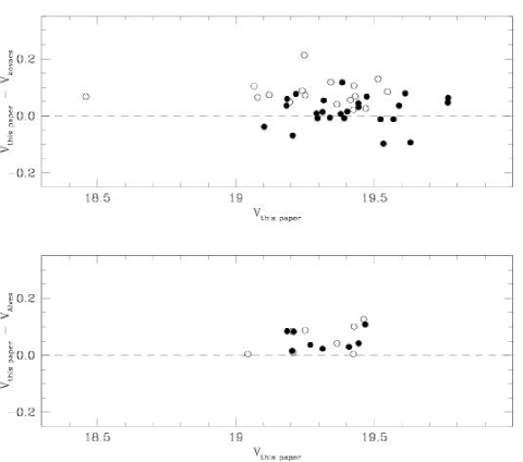
Figure 18: Comparison between our and Kovács (top panel) and Alves (bottom panel) mean $V$ magnitudes for the variable stars in common. Residuals are: this paper $-$ others. Filled and open symbols are used for variable stars in field A and B, respectively.

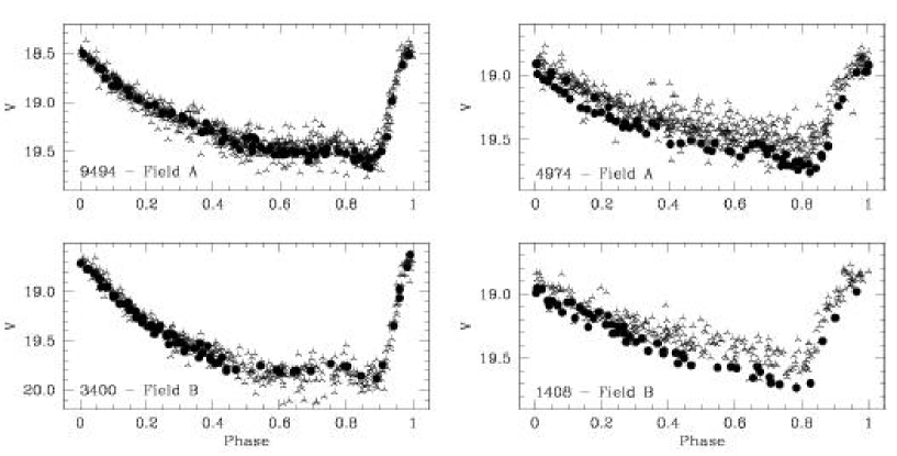
Figure 19: Point-to-point comparison of the light curves for ab-type RR Lyrae stars in common with Kovács subsample. Filled dots: our photometry, three arms crosses: MACHO photometry. These represent the best (left) and worst (right) cases.

Table 10: Comparison with MACHO photometry for the variable stars in common: Kovács subsample

IdMACHO	Id${}_{this\leavevmode\nobreak\ paper}$	$<V_{MACHO}>$	$<V_{this\leavevmode\nobreak\ paper}>$	$<V_{Kovacs}>$	$<V_{this\leavevmode\nobreak\ paper}>$	$\Delta 1$	$\Delta 2$	Field
		(mag-averaged)	(mag-averaged)	(int-averaged)	(int-averaged)
6.6931.603	2525	19.636	19.376	19.346	19.340	$-$0.260	$-$0.006	A
6.6932.948	4974	19.499	19.406	19.267	19.384	$-$0.093	0.117	A
6.6811.882	6398	19.526	19.347	19.263	19.317	$-$0.179	0.054	A
6.6811.736	6426	19.421	19.227	19.125	19.185	$-$0.194	0.060	A
6.6813.923	9494	19.483	19.266	19.140	19.217	$-$0.217	0.077	A
6.6934.1136	9660	19.615	19.407	19.400	19.392	$-$0.208	$-$0.008	A
6.6810.635	12896	19.807	19.620	19.554	19.589	$-$0.187	0.035	A
6.6691.1079	25301	20.006	19.805	19.719	19.766	$-$0.201	0.047	A
6.7054.801	25362	19.656	19.488	19.399	19.443	$-$0.168	0.044	A
6.6692.1042	26525	19.685	19.507	19.406	19.473	$-$0.178	0.067	A
13.5956.410	1408	19.288	19.369	19.225	19.343	0.081	0.118	B
13.5835.395	1575	19.262	19.290	19.177	19.250	0.028	0.073	B
13.6078.524	3054	19.084	19.089	18.962	19.066	0.005	0.104	B
6.6931.817	3061	19.983	19.679	19.724	19.631	$-$0.304	$-$0.093	A
13.5957.489	3400	19.607	19.530	19.443	19.469	$-$0.077	0.026	B
13.6199.527	3412	19.596	19.460	19.403	19.425	$-$0.136	0.022	B
6.7053.758	3805	19.567	19.415	19.387	19.402	$-$0.152	0.015	A
6.6811.752	3948	19.497	19.331	19.283	19.292	$-$0.166	0.009	A
13.5837.629	4540	19.443	19.450	19.358	19.414	0.007	0.056	B
13.5837.382	4859	19.278	19.294	19.152	19.240	0.016	0.088	B
6.6811.591	4933	19.387	19.127	19.141	19.103	$-$0.260	$-$0.038	A
13.5837.566	5902	19.169	19.165	19.047	19.121	$-$0.004	0.074	B
13.6079.125	5952	18.444	18.463	18.392	18.459	0.019	0.067	B
6.7054.713	6415	19.436	19.215	19.275	19.206	$-$0.221	$-$0.069	A
13.5838.576	6440	19.133	19.280	19.038	19.247	0.147	0.213	B
13.6201.449	7063	19.195	19.213	19.147	19.195	0.018	0.048	B
6.7054.582	7477	19.408	19.249	19.148	19.183	$-$0.159	0.035	A
6.7054.373	7609	19.617	19.340	19.299	19.313	$-$0.277	0.014	A
13.6080.435	7620	19.108	19.133	19.014	19.079	0.025	0.065	B
6.6933.1036	8788	19.706	19.482	19.413	19.444	$-$0.224	0.031	A
6.6933.953	9154	19.780	19.569	19.534	19.522	$-$0.211	$-$0.012	A
6.6813.1071	10487	19.838	19.603	19.581	19.569	$-$0.235	$-$0.012	A
13.6078.615	10692	19.568	19.574	19.463	19.548	0.006	0.085	B
13.6078.672	10811	19.538	19.492	19.363	19.431	$-$0.046	0.068	B
6.6931.779	10914	19.853	19.784	19.704	19.767	$-$0.069	0.063	A
13.5957.581	14449	19.459	19.450	19.385	19.514	$-$0.009	0.129	B
6.6690.904	15387	19.814	19.630	19.533	19.612	$-$0.184	0.079	A
6.6811.969	16249	19.674	19.430	19.372	19.379	$-$0.244	0.007	A
13.6080.645	22917	19.439	19.462	19.321	19.427	0.023	0.106	B
13.6080.584	24089	19.450	19.370	19.324	19.365	$-$0.080	0.041	B
6.7055.830	26933	19.597	19.355	19.303	19.295	$-$0.242	$-$0.008	A
6.7055.1045	28539	19.945	19.592	19.631	19.533	$-$0.353	$-$0.098	A

The comparison between MACHO mean V magnitudes and our magnitude-averaged values (see column 11 of tables 5 and 6) for variables in common with full coverage of the light curve and without systematic shifts between the 1999 and the 2001 photometries is shown in Figure 17, where filled and open symbols are used for variables in field A and B, respectively, and triangles mark the double mode RR Lyrae stars. The average $V$ difference, present photometry minus MACHO, is $-0.170$ mag ($\sigma=0.106$, 66 stars) in field A, and $-0.013$ mag ($\sigma=0.099$, 44 stars) in field B. While there is very good agreement for stars in field B, there is a large systematic shift for the variables in field A, with MACHO web luminosities being on average fainter than ours by 0.170 mag. We thus suspect that there may be calibration problems, namely disalignements and photometric shift between different fields, affecting the individual average magnitudes published on MACHO web catalogue for the LMC variable stars. On the other hand we also note that Alcock et al. (2000: hereinafter A00) median luminosity of a sub-sample of 680 RRab’s in the LMC ($<V>$=19.45 mag) is in good agreement, within the respective error bars, with the average luminosity of the RR Lyrae stars in the LMC drawn from the present photometry (see discussion in Section 6 of C03 and their Table 5).

4.2.2 Comparison with MACHO photometry for the variable stars: Kovács subsample

MACHO time series calibrated data for a subsample of 42 variables in common with our photometry (39 RRab, 1 RRc, 1 AC and 1 eclipsing binary, according to our classification; 41 RRab and 1 RRL+GB according to MACHO) were kindly provided to us by Dr. G. Kovács.

This photometry is based on A99 calibration. The comparison between mean magnitudes is shown in the top panel of Figure 18. Individual values are provided in Table 10, where we list MACHO’s web page magnitude-averaged values (Column 3), the present paper magnitude-averaged values (Column 4), and the intensity-averaged values from our photometry and Kovács dataset in Column 5 and 6, respectively. Finally, in Columns 7 and 8 we list the corresponding residuals this paper minus MACHO web ($\Delta$1), and this paper minus Kovács ($\Delta$2). The agreement with Kovács dataset is generally good and without apparent offsets between field A and B. The average difference $\Delta 2$=$<V_{this\leavevmode\nobreak\ paper}>-<V_{Kovacs}>$ is 0.043 mag ($\sigma$=0.059, 42 stars), to compare with $<\Delta 1>$=$<V_{this\leavevmode\nobreak\ paper}>-<V_{MACHO\leavevmode\nobreak\ web}>$ = $-$0.123 mag ($\sigma$=0.120, 42 stars). Our average magnitudes are generally fainter than Kovács’ as expected on the basis of the different reduction procedures (see dicussion in Section 4.1). Figure 19 shows the point-to-point comparison of the light curves of 4 ab-type RR Lyrae stars (two per each of our fields) representing respectively the best (left panels) and the worst (right panels) comparison between the two samples. The two variables shown in the right panels of the figure are systematically brighter in MACHO photometry.

Table 11: Comparison with MACHO photometry for the variable stars in common: Alves subsample

IdMACHO	Id${}_{this\leavevmode\nobreak\ paper}$	$<V_{MACHO}>$	$<V_{this\leavevmode\nobreak\ paper}>$	$<V_{Alves}>$	$<V_{this\leavevmode\nobreak\ paper}>$	TypeMACHO	Type${}_{this\leavevmode\nobreak\ paper}$
		(mag-averaged)	(mag-averaged)	(int-averaged)	(int-averaged)
6.6931.650	2767	19.602	19.517	19.359	19.467	RRab	RRab
6.6810.428	3155	19.338	19.218	19.127	19.209	RRc	RRd
13.6691.4052	4420	19.402	19.417	19.380	19.409	$-$	RRd
6.6811.736	6426	19.421	19.227	19.101	19.185	RRab	RRab
13.7054.2970	7137	19.150	$-$	19.309	19.413	RRd	RRd
6.7054.373	7609	19.617	19.340	19.290	19.313	RRab	RRab
6.6933.939	8654	19.440	19.275	19.233	19.269	RRe	RRd
6.6933.1036	8788	19.706	19.482	19.402	19.444	RRab	RRab
6.6692.853	10214	19.440	19.217	19.189	19.204	RRab	RRab
13.5835.395	1575	19.262	19.290	19.163	19.250	RRab	RRab
13.6078.524	3054	19.084	$-$	18.953	19.066	RRab	RRab
13.5836.525	3347	19.145	19.211	19.120	19.204	RRc	RRd
13.6199.527	3412	19.596	19.460	19.422	19.425	RRab	RRab
13.5958.518	4509	19.210	19.468	19.336	19.462	RRd	RRd
13.5838.497	6470	19.224	19.218	19.197	19.207	RRc	RRd
13.6080.591	7467	19.076	19.055	19.040	19.043	RRc	RRd
13.6080.645	22917	19.439	19.462	19.327	19.427	RRab	RRab
13.6080.584	24089	19.450	19.370	19.323	19.365	RRab	RRab

Notes: Stars # 7137 and # 4509 do not appear in the MACHO on-line catalogue, values in Column 3 for these stars are taken from A97 (see their Table 1).

4.2.3 Comparison with MACHO photometry for the variable stars in common: Clement subsample

Alcock et al. (2004) discuss the properties of 330 first-overtone M5-like RR Lyrae variables contained in 16 LMC MACHO fields including fields #6 and # 13. These restricted sample includes MACHO “best-fit” c-type RR Lyrae with $-0.56<\log P<-0.4$, amplitudes $A_{V}>0.3$ and amplitude ratios in the range $0.75<A_{R}/A_{V}<0.85$ (C. Clement private communication, Alcock et al. 2004). Photometry of these stars is based on version 9903018 of A99 calibration (Alcock et al. 2004). Seven of these RRc’s are in our sample: we find that MACHO’s mean magnitudes are on average 0.07 mag brighter than ours (see Table 12 by Alcock et al. 2004), again as expected on the basis of the different reduction procedures. This shift is totally consistent with that found from the larger sample of newly calibrated MACHO light curves provided us by D. Alves (see following Section 4.2.4), but at odds with the results from the comparison with the MACHO web values. We explicitely notice that this is indeed a small sample, since it was selected as described above, but as discussed in Section 4.2.1, and contrary to what stated by Alves (2004), we have a much larger number of variable stars in common with MACHO database.

4.2.4 Comparison with MACHO photometry for the variable stars in common: Alves subsample

Dr. D. Alves kindly made available to us time series data for a subsample of 18 RR Lyrae variables in common with our database (9 for each field, 10 RRab and 8 RRd according to our classification; 10 RRab, 4 RRc, 2 RRd, 1 RRe and 1 variable of unknown type according to MACHO, but classified RRd by A97) along with photometry for the non-variable stars falling in $\sim 4^{\prime}\times 4^{\prime}$ patches surrounding these RR Lyrae stars. These photometric data are calibrated according to A99 and Alcock et al. (2004) calibrations (Alves 2004, private communication). Counteridentifications and average magnitudes of these 18 stars are given in Table 11. The comparison between intensity-averaged magnitudes is generally good, (see columns 5 and 6 of Table 11 and bottom panel of Figure 18), with Alves values being 0.061 mag brighter ($\sigma=0.042$, 18 stars) than ours and without significant differences between field A and B. The corresponding comparison using the magnitude-averaged luminosities of these RR Lyrae stars available on MACHO web pages leads to a different result: MACHO web values are on average 0.067 mag fainter than ours (see Columns 3 and 4 of Table 11).

4.2.5 Comparison with MACHO photometry for the non-variable stars: Alves subsample

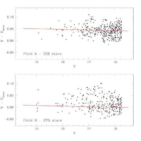
Figure 20: Comparison with MACHO photometry (Alves subsample) for non-variable stars brighter than 18.25 mag. Residuals are this paper minus MACHO. Lines indicate the linear fits of the average residuals of all bins.

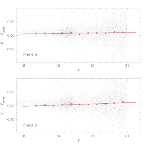
Figure 21: Same as Figure 20 for non-variable with $18.25<V<21$ mag.

Table 12: Comparison with MACHO photometry for the non-variable stars with $V<18.25$, from Alves subsample

Bin	$<\Delta V>$	$\sigma$	N
Field A
15.00 $-$ 17.00	0.045	0.021	64
17.00 $-$ 17.25	0.055	0.031	34
17.25 $-$ 17.50	0.043	0.011	31
17.50 $-$ 17.75	0.037	0.027	58
17.75 $-$ 18.00	0.038	0.021	81
18.00 $-$ 18.25	0.045	0.025	88
Field B
15.00 $-$ 17.00	0.026	0.029	61
17.00 $-$ 17.25	0.022	0.037	36
17.25 $-$ 17.50	0.027	0.041	29
17.50 $-$ 17.75	0.011	0.031	30
17.75 $-$ 18.00	0.012	0.029	57
18.00 $-$ 18.25	0.010	0.022	62

Notes: $<\Delta V>$ = $<V_{this\leavevmode\nobreak\ paper}-V_{Alves}>$

Table 13: Comparison with MACHO photometry for the non-variable stars with $18.25<V<21$, from Alves subsample

Bin	$<\Delta V>$	$\sigma$	N
Field A
18.25 $-$ 18.50	0.030	0.027	123
18.50 $-$ 18.75	0.032	0.030	133
18.75 $-$ 19.00	0.024	0.031	188
19.00 $-$ 19.25	0.035	0.037	502
19.25 $-$ 19.50	0.037	0.042	673
19.50 $-$ 19.75	0.013	0.049	329
19.75 $-$ 20.00	0.035	0.063	327
20.00 $-$ 20.25	0.035	0.065	445
20.25 $-$ 20.50	0.033	0.098	603
20.50 $-$ 20.75	0.054	0.110	753
20.75 $-$ 21.00	0.045	0.129	826
Field B
18.25 $-$ 18.50	0.001	0.030	98
18.50 $-$ 18.75	0.012	0.034	115
18.75 $-$ 19.00	$-0.001$	0.032	164
19.00 $-$ 19.25	0.014	0.040	438
19.25 $-$ 19.50	0.028	0.055	426
19.50 $-$ 19.75	0.019	0.060	268
19.75 $-$ 20.00	0.017	0.057	280
20.00 $-$ 20.25	0.020	0.074	373
20.25 $-$ 20.50	0.027	0.087	466
20.50 $-$ 20.75	0.041	0.119	647
20.75 $-$ 21.00	0.057	0.116	694

Notes: $<\Delta V>$ = $<V_{this\leavevmode\nobreak\ paper}-V_{Alves}>$

The non-variable stars in common were counteridentified by coordinates. They correspond to a total number of 18996 stars (10467 in field A, and 8529 in field B, respectively).

Comparison between the two photometries was done dividing the stars into a bright and a faint sample corresponding respectively to objects with $V<18.25$ mag (356 stars in field A, and 275 in field B) and objects with $18.25<V<21$ mag (4902 stars in field A, and 3969 in field B). Within each subsample stars where further divided into magnitude bins 0.25 mag wide. Average residuals were computed adopting a $\sigma$ rejection procedure that discarded objects deviating more than 2 $\sigma$ from the average in the bin. In Table 12 we list the mean differences $V_{this\leavevmode\nobreak\ paper}$ $-V_{Alves}$ of the stars in the bright subsample (for objects in field A and B separately), with their respective $\sigma$ and number of stars per magnitude bin. Transformation equations between the two photometries were then computed as the linear fit of the average residuals of all bins. They are:

$$V_{this\leavevmode\nobreak\ paper}-V_{Alves}=-0.0028\times V_{this\leavevmode\nobreak\ paper}+0.0916$$

in field A (356 objects) and:

$$V_{this\leavevmode\nobreak\ paper}-V_{Alves}=-0.0025\times V_{this\leavevmode\nobreak\ paper}+0.0438$$

in field B (275 stars). These linear fits are shown in Figure 20.

The same comparison done on the stars with $18.25<V<21$ mag is provided in Table 13 and shown in Figure 21. The transformation equations in this magnitude range using a linear fit with a 2 $\sigma$ rejection are:

$$V_{this\leavevmode\nobreak\ paper}-V_{Alves}=0.0067\times V_{this\leavevmode\nobreak\ paper}-0.0953$$

in field A (4902 objects) and:

$$V_{this\leavevmode\nobreak\ paper}-V_{Alves}=0.0177\times V_{this\leavevmode\nobreak\ paper}-0.3251$$

in field B (3969 stars).

4.3 Comparison with OGLE II photometry

The partial overlap of our field A with OGLE II field LMC_SC21 (Udalski et al. 2000) gave us the possibility to make a detailed comparison between the two photometries based on a large number of stars covering a wide magnitude range. We have retrieved from the OGLE archive the photometric data corresponding to field LMC_SC21. The overlapping region corresponds to 42.25% and 9.84% of our and OGLE II fields, respectively. This region is located at roughly 5:21:29.9 $<\alpha<$ 5:22:38.6 and $-$70:41:00.9 $<\delta<-$ 70:27:18.4, corresponding to 1218.95 $<X<$ 2047.44 and 2976.78 $<Y<$ 4967.58 in OGLE II coordinate system. Inside this area OGLE II has $B$,$V$,$I$ photometry for 15524, 17067 and 17582 stars, respectively, to compare with our 21524 objects. Our limiting magnitude is about 1.5 mag fainter and we resolved about 39, 26, and 22% more stars (in $B$, $V$ and $I$, respectively) than OGLE II. Coordinates were aligned to OGLE II coordinate system and stars in common were counteridentified. Over the total sample of 14734 common stars there are 13688, 14483 and 14734 objects with $B$, $V$ and $I$ magnitude in the ranges 12.5$-$22.7, 12.6$-$23.1 and 12.3$-$21.6, respectively. Among these objects OGLE II reports 39 variable stars. We recovered all of them. Counteridentifications are provided in Table 14 along with average luminosities and classification in types in the two photometries. There is general agreement in the type classification and in the derived periods that, on average, agree within 2-3 decimal digits. OGLE II classification does not match ours for 4 variable stars, namely the new candidate RRd, 2 candidate Anomalous Cepheids and star # 5148 that we classify as RRab while is classified RRc by OGLE II. A further object, star Id_{SC_21} =116626 is classified by OGLE II as CepFA; however, OGLE II light curves for this star are rather poor and the corresponding object in our photometry (# 22592) was not found to vary. Finally, we have three additional variables in the area in common that were apparently missed by OGLE II: an RRc, a binary system, and a $\delta$ Scuti star, which are listed at the bottom of Table 14. For 3 variables (namely stars # 9604, 10320, and 25510) there is a large discrepancy between OGLE II and our $V$ average magnitudes. Two of these stars (# 9604 and 10320) were discussed in Section 3.2. Similarly to them, star # 25510 has a very poor $V$ light curve in OGLE II photometry and an average $V$ magnitude 0.62 mag fainter than ours, leading to unrealistic $<B-V>$=$-$0.11 and $<V-I>$=1.04 colours for an RR Lyrae star. We suspect that these 3 stars may have been wrongly counteridentified in the various photomeric bands. Figure 22 shows the point-to-point comparison of the $V$ light curves for 3 ab-type RR Lyrae stars and one Cepheid representing respectively the best agreement (left panels) and the worst (right panels) comparison between the two photometries (excluding the 3 above mentioned discrepant stars). Large discrepancies are also found among the $B$ magnitudes of stars # 4313 and 8723, that, in the case of the first object, lead in OGLE II photometry to a colour $<B-V>$=0.85 mag rather red for an RR Lyrae star.

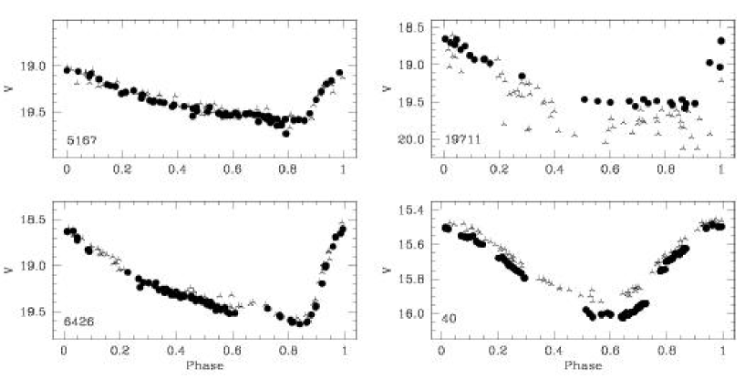
Figure 22: Point-to-point comparison of the $V$ light curves for 3 ab-type RR Lyrae stars and a Classical Cepheid (lower right panel) in common with OGLE II. Filled dots: our photometry, three arms crosses: OGLE II photometry. As in Figure 19, these represent the best (left) and worst (right) cases.

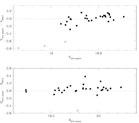
Figure 23: Comparison between our and Ogle II mean $V$ and $B$ magnitudes for the variable stars in common. Residuals are: this paper $-$ OGLE II. Open symbols are used for the most deviating stars (see text).

The comparison between our and OGLE II mean $V$,$B$ magnitudes for variable stars in common with complete light curves and no systematic shifts between our 1999 and 2001 photometry is shown in Figure 23. Average differences are $\Delta V$=0.01 mag ($\sigma=0.11$, 30 stars discarding stars # 9604, 10320 and 25510, open circles in Figure 23) and $\Delta B$=0.04 mag ($\sigma=0.15$, 29 stars, discarding also star # 19711 that does not have $B$ magnitude in OGLE-II), respectively. These average differences do not change restricting the comparison only to the RR Lyrae stars. Our photometry is on average slightly fainter than OGLE-II, again as expected on the basis of the different reduction procedures used in the two photometries (see Section 4.1). The average $V$ magnitude of the RR Lyrae stars in common using objects with reliable photometry in both datasets is $<V_{RR}>$=19.444 mag ($\sigma=0.181$, 24 stars) and $<V_{RR}>$=19.427 mag ($\sigma=0.160$, 24 stars) in our and OGLE-II photometry, respectively. These values are in good agreement with each other and with the average $V$ luminosity of our full sample of RR Lyrae stars in field A (see end of Section 3.1 and C03), but about 0.06-0.08 mag fainter than the average $V$ magnitude from the total sample of OGLE II LMC RRab’s: $<V_{RR}>$=19.36$\pm$0.03 mag (and $<V_{RR}>$=19.31$\pm$0.021 mag for the RRc’s) by Soszyńsky et al. (2003). Given the small sample of variable stars in common this systematic shift might appear not very statistically significant, however it is fully confirmed by the comparison done on the much larger number of non variable stars at the same magnitude level (see remaining part of this section and Table 15).

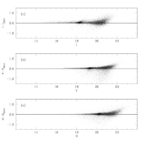
Figure 24: Comparison between our and OGLE II photometry for the about 14,000 stars in common. Residuals are this paper minus OGLE II.

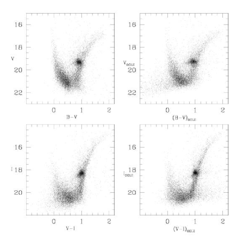
Figure 25: $V\,vs\,(B-V)$ and $V\,\textit{vs\,}(V-I)$ CMDs for the stars in common between our field A and OGLE II field LMC_SC21. Left panels: this paper; right panels: OGLE II.

$B$, $V$ and $I$ residuals between our and OGLE II photometry for the non variable stars in common are shown in Figure 24, while in Figure 25 we plot the corresponding CMDs (left panels: present paper; right panels: OGLE II photometry). Our $B$,$V$ photometry is generally more accurate and deeper than OGLE’s. Objects falling off the main ridge lines of OGLE II  $V,B-V$ CMD for $V>20.0$ and $(B-V)<$0.2 are likely wrong measurements in OGLE II photometry (e.g., blends, wrong identifications, and wrong counteridentifications between $V$ and $B$) since they fall very well on the main branches of our diagram. In the $I$ band our photometry appears to be more uncertain. However, the objects that deviate most in our $I$ photometry ($I>20.0$ and $V-I<$ 0.0) have magnitudes generally well below the magnitude level of RR Lyrae and clump stars, that are the luminosity levels we are mainly interested in.

Table 14: Variable stars inside the area in common with OGLE II field LMC_SC21.

Name	Type	Id	$<V>$	$<B>$	$<I>$	Id	Type	$<V>$	$<B>$	$<I>$	$\Delta V$	$\Delta B$
OGLE	OGLE	SC_21	OGLE	OGLE	OGLE	${}_{this\leavevmode\nobreak\ paper}$	${}_{this\leavevmode\nobreak\ paper}$	${}_{this\leavevmode\nobreak\ paper}$	${}_{this\leavevmode\nobreak\ paper}$	${}_{this\leavevmode\nobreak\ paper}$
OGLE052133.45-703951.6	RRc	111870	19.29	19.57	18.90	2249	RRdm	19.372	19.704	18.878	0.08	0.13
OGLE052130.54-703711.5	RRab	112191	19.48	20.01	18.86	15387	RRab	19.612	20.043	$-$	0.13	0.03
OGLE052131.78-703646.5	RRc	114344	19.48	19.77	18.99	4388	RRc	19.427	19.758	$-$	$-$0.05	$-$0.01
OGLE052148.39-703026.1	CepFU	116226	16.12	16.67	15.46	183	Cep	16.259	16.830	15.566	0.14	0.16
OGLE052134.12-703024.8	RRab	116880	19.72	20.15	19.02	25301	RRab	19.766	20.237	$-$	0.05	0.09
OGLE052133.57-703157.5	RRdm	117174	19.45	19.91	18.99	23032	RRdm	19.597	19.993	$-$	0.15	0.08
OGLE052148.90-702801.2	RRc	119123	19.44	19.27	17.91	10320	AC	18.655	19.236	$-$	$-$0.79	$-$0.03
OGLE052154.07-702917.8	RRab	119283	19.58	20.09	18.92	26821	RRab	19.624	20.097	19.097	0.04	0.01
OGLE052146.25-702813.5	RRab	119434	19.46	19.96	18.76	28293	RRab	19.520	20.053	$-$	0.06	0.09
OGLE052131.26-702812.2	RRab	119439	19.21	19.63	18.59	10214	RRab	19.204	19.639	$-$	$-$0.01	0.01
OGLE052152.61-702929.0	RRab	119754	19.45	19.86	18.93	26525	RRab	19.473	19.913	$-$	0.02	0.05
OGLE052212.39-704010.0	CepFO	159587	15.69	16.18	15.07	40	Cep	15.753	16.237	15.212	0.06	0.06
OGLE052235.42-703828.6	RRdm	160118	19.23	19.51	18.68	3155	RRdm	19.209	19.577	18.792	$-$0.02	0.07
OGLE052157.21-703826.1	RRe	160121	19.22	19.54	18.68	3216	RRc	$-$	$-$	$-$	$-$	$-$
OGLE052222.37-704000.1	RRe	160409	19.70	20.11	19.32	2119	RRc	19.659	19.986	19.407	$-$0.04	$-$0.12
OGLE052216.65-703950.4	RRc	160428	19.48	19.79	19.06	2223	RRc	19.556	19.836	19.136	0.08	0.05
OGLE052230.17-703553.8	RRab	162785	19.24	19.63	18.60	4933	RRab	19.103	19.531	18.542	$-$0.14	$-$0.10
OGLE052159.82-703535.3	RRab	162827	19.35	19.77	18.68	5167	RRab	19.359	19.837	18.808	0.01	0.07
OGLE052221.06-703534.2	RRc	162831	19.02	19.41	18.40	5148	RRab	$-$	$-$	$-$	$-$	$-$
OGLE052209.71-703502.8	RRab	162907	19.52	20.02	18.86	5589	RRab	19.574	20.079	18.942	0.05	0.06
OGLE052232.64-703348.9	RRab	163060	19.15	19.57	18.57	6426	RRab	19.185	19.584	18.555	0.04	0.01
OGLE052208.39-703631.3	RRab	163171	19.38	19.67	18.77	16249	RRab	19.379	19.671	$-$	0.00	0.09
OGLE052238.32-703402.1	RRab	163532	19.49	$-$	18.72	19711	RRab	19.200	19.535	18.607	$-$0.29	$-$
OGLE052210.67-703315.2	CepFU	165209	16.23	16.83	15.48	150	Cep	16.251	16.837	15.524	0.02	0.01
OGLE052221.29-703244.2	RRab	165596	19.37	19.84	18.83	7211	RRab	$-$	$-$	$-$	$-$	$-$
OGLE052230.18-703220.8	RRab	165650	19.52	20.07	18.83	7468	RRab	19.615	20.127	18.850	0.10	0.06
OGLE052207.98-703200.1	RRab	165710	19.43	20.06	18.79	7734	RRab	$-$	$-$	$-$	$-$	$-$
OGLE052226.55-703019.3	RRc	165913	19.46	19.77	18.89	8812	RRc	19.397	19.767	18.821	$-$0.06	$-$0.00
OGLE052213.53-703011.8	RRab	165930	19.77	19.66	18.73	25510	RRab	19.150	19.614	18.554	$-$0.62	$-$0.05
OGLE052229.04-703036.1	RRc	166393	19.49	19.82	19.01	8622	RRc	19.542	19.868	19.103	0.05	0.05
OGLE052207.18-702907.7	RRab	168608	19.66	19.21	18.45	9604	AC	18.932	19.234	18.550	$-$0.73	0.02
OGLE052214.15-702835.3	RRc	168696	19.25	19.53	18.71	27697	RRc	19.166	19.541	$-$	$-$0.08	0.01
OGLE052224.72-702740.8	RRab	168833	19.49	19.77	18.89	10487	RRab	19.569	20.022	18.886	0.08	0.25
OGLE052206.67-702755.9	RRc	169354	19.79	20.01	19.23	28665	RRc	$-$	$-$	$-$	$-$	$-$
OGLE052134.09-703652.8	RRab	111805	19.46	20.31	18.77	4313	RRab	19.270	19.779	18.451	$-$0.19	$-$0.53
OGLE052213.85-700927.2	EB	165895	19.32	19.48	18.81	8723	EB?	19.152	19.859	$-$	$-$0.17	0.38
OGLE052219.01-703311.0	RRab	166016	19.16	19.67	18.73	21007	RRab	19.319	19.841	18.487	0.16	0.17
OGLE052214.83-702807.0	RRab	169311	19.68	20.02	19.06	28246	RRab	19.605	20.030	19.144	$-$0.08	0.01
OGLE052155.09-703212.3	CepFA	116626	19.40	20.42	18.32	22592	(1)	$-$	$-$	$-$ $-$	$-$
OGLE052235.68-702815.9	$-$	169285	$-$	$-$	$-$	28114	$\delta$S	19.940	20.273	$-$	$-$	$-$
OGLE052153.64-703635.4	$-$	114367	$-$	$-$	$-$	4490	EB	19.016	19.011	19.017	$-$	$-$
OGLE052129.44-702923.6	$-$	119268	$-$	$-$	$-$	26715	RRc	19.378	19.725	$-$	$-$	$-$

(1) Star OGLE052155.09-703212.3, ( Id_{SC_21} =116626), is classified by OGLE II as CepFA, however OGLE II light curves for this star are rather poor and the corresponding object in our photometry (# 22592) is not was found to vary.

Table 15: Comparison of our and OGLE II photometry for the non variable stars in common. $<\Delta V>$,$<\Delta B>$,$<\Delta I>$ are: this paper $-$ OGLE II

Bin	$<\Delta V>$	$\sigma_{V}$	N			Bin	$<\Delta B>$	$\sigma_{B}$	N			Bin	$<\Delta I>$	$\sigma_{I}$	N
15.00-17.00	0.045	0.017	64			16.00-17.00	0.014	0.036	16			14.00-15.00	0.063	0.053	35
17.00-17.25	0.044	0.027	60			17.00-17.50	-0.006	0.091	22			15.00-16.00	0.070	0.044	129
17.25-17.50	0.044	0.021	76			17.50-18.00	0.009	0.027	24			16.00-17.00	0.056	0.040	300
17.50-17.75	0.044	0.023	96			18.00-18.25	0.025	0.036	28			17.00-17.50	0.052	0.042	273
17.75-18.00	0.043	0.025	107			18.25-18.50	0.011	0.036	51			17.50-18.00	0.042	0.033	368
18.00-18.25	0.048	0.028	122			18.50-18.75	0.017	0.032	88			18.00-18.25	0.040	0.037	626
18.25-18.50	0.048	0.026	174			18.75-19.00	0.022	0.030	149			18.25-18.50	0.055	0.045	1040
18.50-18.75	0.043	0.021	194			19.90-19.25	0.026	0.034	161			18.50-18.75	0.052	0.049	479
18.75-19.00	0.049	0.026	250			19.25-19.50	0.031	0.038	218			18.75-19.00	0.043	0.054	344
19.00-19.25	0.049	0.030	628			19.50-19.75	0.034	0.030	330			19.00-19.50	0.045	0.062	966
19.25-19.50	0.062	0.032	1105			19.75-20.00	0.032	0.042	524			19.50-19.75	0.027	0.080	723
19.50-19.75	0.069	0.036	579			20.00-20.25	0.026	0.049	1115			19.75-20.00	0.031	0.091	1008
19.75-20.00	0.068	0.044	510			20.25-20.50	0.044	0.047	1125			20.00-20.25	0.035	0.113	1340
20.00-20.25	0.067	0.051	611			20.50-20.75	0.035	0.063	864
20.25-20.50	0.073	0.063	838			20.75-21.00	0.039	0.066	944
						21.00-21.25	0.038	0.082	1046

In order to make a more meaningful comparison of the two photometries we restricted the sample of the stars in common only to objects brighter than $V$=20.5, $B$=21.25, and $I$=20.25 mag. Average residuals were computed dividing the objects in magnitude bins and applying an iterative $\sigma$-rejection procedure which discarded objects deviating more than 3$\sigma$ from the average in the bin. Results are summarized in Table 15 (they are based on 5414, 6705, and 7631 stars in $V,B,I$ respectively). At the magnitude level of RR Lyrae and clump stars ($V\sim 19.4,B\sim 19.8,I\sim 18.8$; and $V\sim 19.3,B\sim 20.2,I\sim 18.3$, respectively) offsets are: $\Delta V$ = 0.06 ($\sigma_{V}$=0.03), $\Delta B$ = 0.03 ($\sigma_{B}$=0.04), $\Delta I$ = 0.04 ($\sigma_{I}$=0.05), and $\Delta V$ = 0.06 ($\sigma_{V}$=0.03), $\Delta B$ = 0.03-0.04 ($\sigma_{B}$=0.05), $\Delta I$ = 0.06 ($\sigma_{I}$=0.05), Our photometry is systematically fainter than OGLE II photometry, again as expected since DoPhot is reported to give systematically brighter magnitudes for faint stars in crowded regions than DAOPHOT/ALLFRAME, and since we resolve many more faint stars than OGLE II in the area in common.

Transformation equations between the two photometries were then computed as linear fits of the average residuals of all the bins:

$$B_{this\leavevmode\nobreak\ paper}-B_{OGLE}=0.00835\times B_{this\leavevmode\nobreak\ paper}-0.13507$$

$$V_{this\leavevmode\nobreak\ paper}-V_{OGLE}=0.00751\times V_{this\leavevmode\nobreak\ paper}-0.08626$$

$$I_{this\leavevmode\nobreak\ paper}-I_{OGLE}=-0.00622\times I_{this\leavevmode\nobreak\ paper}+0.15914$$

Thus the transformation relations between OGLE II and our photometry are:

$$B_{this\leavevmode\nobreak\ paper}=1.0084\times B_{OGLE}-0.1362$$

$$V_{this\leavevmode\nobreak\ paper}=1.0076\times V_{OGLE}-0.0869$$

$$I_{this\leavevmode\nobreak\ paper}=0.9938\times I_{OGLE}+0.1582$$

5 The pulsation characteristics of the RR Lyrae stars

We have detected and derived periods for a total number of 135 RR Lyrae stars in our two fields (78 in field A, and 57 in field B). This number includes 87 fundamental mode (RRab), 38 first overtone (RRc), and 10 double-mode (RRd) pulsators. According to the completness of our photometry and the comparison with MACHO and OGLE II catalogues (Sections 4.2 and 4.3) our sample of variables should be about 97% complete. The two fields are found to contain about the same number of first overtone RR Lyrae (20 in field A and 18 in field B) while the number of fundamental mode pulsators is about 50% larger in field A (52 RRab) than in field B (35 RRab). We found that 17% of the fundamental mode RR Lyraes in our two fields are (or are suspected to be) affected by the Blazhko phase and amplitude modulation of the light curve (Blazhko 1907). This percentage is consistent with the 11.9% and the 15% Blazhko incidence rates among RRab’s reported respectively by MACHO (Alcock et al. 2003b) and OGLE II (Soszyńsky et al. 2003), and maybe closer to the 20%-30% incidence rate commonly found for the Milky Way fundamental mode RR Lyrae (Szeidl 1988, Moskalik & Poretti 2003). The first-overtone Blazhko variables are the 5.3% of our RRc sample, again in agreement with both MACHO ($\sim$ 4%, Alcock et al. 2003b), and OGLE II ($\sim$ 6%, Soszyńsky et al. 2003).

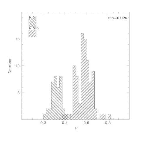
Figure 26: Number vs Period histogram of the single-mode RR Lyrae variables in our sample (125 objects).

Figure 26 shows the period distribution of the single-mode RR Lyrae’s (125 objects). The two peaks correspond to the average period of the c- and ab-type pulsators, respectively: $<{\rm P_{RR_{c}}}>$=0.324 days ($\sigma$=0.048, 38 stars) and $<{\rm P_{RR_{\rm ab}}}>$=0.581 days ($\sigma$=0.071, 87 stars), to compare with 0.342 and 0.583 day of A96, and with 0.339 and 0.573 days by Soszyńsky et al. (2003). Our average periods are in good agreement with both A96 and Soszyńsky et al. (2003) results, which are based on much larger samples, and confirm that the average period of the ab-type variables of the LMC is intermediate between the periods of the Galactic RR Lyrae stars of Oosterhoff type I (OoI) and II (OoII), but it is actually closer to the Oo I clusters (being $<$P${}_{{\rm RR_{\rm ab}}}>$=0.55, and 0.65 days in Oo I and II clusters, respectively; Oosterhoff 1939). Our results also indicate that the average pulsation properties of the RR Lyrae stars in the two fields are slightly different, with variables in field B being more definitely of Oo type I. Field B contains in fact a larger number of ab-type RR Lyrae with periods around half a day (10 out of 35 RRab’s in field B have P=0.50$\pm$0.02 days corresponding to 28.6 %, while only 5 out of 52 in field A, corresponding to 9.6 %), as confirmed by the average periods computed keeping the variables in the two fields separate. These are: $<{\rm P_{RR_{c}}}>$=0.320$\pm 0.011$ days ($\sigma$=0.050, 20 stars), $<{\rm P_{RR_{\rm ab}}}>$=0.593$\pm 0.010$ days ($\sigma$=0.065, 52 stars), and $<{\rm P_{RR_{c}}}>$=0.329$\pm 0.011$ days ($\sigma$=0.047, 18 stars), $<{\rm P_{RR_{\rm ab}}}>$=0.562 $\pm 0.013$ days ($\sigma$=0.075, 35 stars), in field A and B, respectively.

The $B$ and $V$ amplitudes (A_B, A_V, see Columns 14 and 15 of Tables 5 and 6) were used together with the newly derived periods to build the period - amplitude diagrams shown in Figure 27. The overlap in the transition region between ab and c-type RR Lyrae is small (5 objects, see Figure 26). Our shortest period ab-type RR Lyrae’s are: star #19450 in field A, P=0.398 days, A_V=1.344 and A_B=1.709 mag; and star #19037 in field B, P=0.411 days, A_V=1.466 and A_B=1.821 mag. The longest period c-types are: star #6415 in field A, with P=0.443 days, A_V=0.438 and A_B=0.473 mag, and stars # 6957 and # 7064 in field B, respectively with P=0.406 days, A_V=0.396, A_B=0.568 mag and P=0.401 days, A_V=0.474, A_B=0.607 mag. These stars define the transition region between ab and c-type RR Lyrae stars that, in our sample, occurs at P${}_{\rm tr}\sim$ 0.40 days, (P_tr = 0.457 days in A96). They are labelled in the period-amplitude distributions in Figure 27.

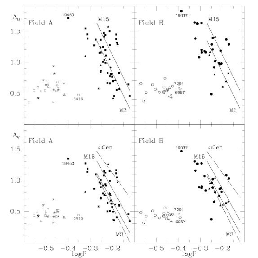
Figure 27: A${}_{B}{\it vs}\log{\rm P}$ and A${}_{V}{\it vs}\log{\rm P}$ diagrams for the RR Lyrae’s with complete $B$ and $V$ light curves in field A and B, separately. Solid lines show the distributions defined by the ab-type RR Lyrae variables in the globular clusters M3 from the photometry of Carretta et al. (1998), and M15 from Bingham et al. (1984). Dashed lines in the lower panels are the A${}_{V}vs\log P$ relations derived for M3 and $\omega$ Cen by Clement (2000) only using RRab’s with regular light curves. Different symbols refer to ab (filled square and circles, in field A and B respectively), c (open square and circles in field A and B respectively), d-type (asterisks) RR Lyrae variables, and candidate Anomalous Cepheids (crosses), respectively. Triangles mark the RR Lyrae variables that are found or sospected to be affected by Blazhko effect. Labels identify RR Lyrae stars at the transition period between ab- and c-types

A96 discuss at some length the existence in their period and amplitude distributions (see figs. 1 and 6 of A96) of an extra-large number of variables with period around 0.28 days, which have asymmetric light curves, but low amplitudes. A96 classify these variables as possible second-overtone RR Lyrae’s (type e), and see also the discussion in Soszyńsky et al. (2003). Figure 26 does not show clear evidence for an extra peak around P$\sim$0.28 days. We have 8 objects in the period range from 0.265 to 0.291 days (4 in each of the two fields). Only two of them show asymmetric light curves, namely: star #2223 in field A with P=0.288 days, A_V=0.493 mag, A_B=0.604 mag, and A_I=0.499 mag; and star #10585 in field B with P=0.270 days, A_V=0.478 mag, and A_B=0.657 mag. Another RRc of slightly longer period has very asymmetric curves: star #7490 in field B with P=0.305 days, A_V=0.505 and A_B=0.637.

The A${}_{V}-\log{\rm P}$, A${}_{B}-\log{\rm P}$ distributions of the variables in the two fields are similar (see Figure 27), and resemble fig. 6 of A96, however our A_V amplitudes range is slightly larger than in A96, with A_V values from 0.29 to 1.47 mag in our sample to compare with 0.35-1.35 in A96.

The period - amplitude distributions of the LMC variables were compared with the relations defined by the ab-type RR Lyrae’s in the globular clusters M3, M15 and $\omega$ Cen, shown by lines in Figure 27. Solid lines were derived from the photometry of Carretta et al. (1998) for M3, and Bingham et al. (1984) for M15, and were computed as follow: we first derived the period-amplitude relations using the M3 sample which is more extended; then we shifted the intercept of these relations while holding fixed the slopes, until a good fit (by eye) was obtained also for the variables in M15, which are too few in number to give a satisfactory best fit by themselves. Dashed lines in the lower panels of Figure 27 are the A${}_{V}vs\log P$ relations derived for M3 and $\omega$ Cen by Clement (2000) using only RRab’s with regular light curves (see also Clement & Shelton 1999, and Clement & Rowe 2000).

RR Lyrae’s in field B seem to better follow the amplitude-period relations of the variables in M3 and, as already noted, to belong to the OoI type. Variables in field A, instead, have pulsation properties more intermediate between the two Ooostheroff types.

5.1 The double-mode pulsators in our sample

According to A97, nine double-mode RR Lyrae stars were expected to fall in the observed areas. We detected all of them and also found evidence for one possible additional RRd: star # 2249. This variable is tentatively classified as d-type mainly because of the large scatter of the observed V and B light curves (0.12 and 0.11 mag, respectively), which has no obvious explanation since the object, although rather faint, is not blended to other stars on the frames. We fully covered the light variation of all RRd’s in our sample; however our sampling of their light curves is too coarse to allow a firm identification of the two periodicities, particularly for stars with fundamental periods around half a day. Periods from A97 have been adopted to phase the data of these variables, apart from star # 2249 for which we use our period.

The average luminosity we derive from the 10 RRd’s in our sample, using the magnitude-averaged values in column 11 of Tables 5 and 6 ($<V_{RRd}>$=19.335 $\pm$0.056, $\sigma$=0.176, 10 stars) is in very good agreement with A00 average luminosity of the LMC double mode RR Lyrae stars ($<V_{RRd}>$=19.327 $\pm$0.021).

We may compare the average luminosity of the RRd variables with the average luminosity of the single-mode RR Lyrae stars in our two fields. Due to the difference in reddening between the two fields (see C03) this comparison is better done keeping the variables in the two areas separated. We found $<V(RRd)>_{FieldA}$ = 19.378$\pm$0.055 ($\sigma$=0.135), and $<B(RRd)>_{FieldA}$=19.731$\pm$0.058 ($\sigma$=0.141) from the average of the 6 RRd’s in field A, to compare with average values derived from the single-mode pulsators of 19.421$\pm$0.020 ($\sigma$=0.156, 61 stars), and 19.824$\pm$0.022 ($\sigma$=0.173, 61 stars), respectively; and $<V(RRd)>_{FieldB}$ = 19.229$\pm$0.087 ($\sigma$=0.173) and $<B(RRd)>_{FieldB}$=19.578$\pm$0.093 ($\sigma$=0.186) from the average of the 4 RRd’s in field B, to compare with average values derived from the single-mode pulsators of 19.326$\pm$0.023 ($\sigma$=0.155, 45 stars), and 19.687$\pm$0.023 ($\sigma$=0.156, 45 stars), respectively. The RRd pulsators seem to be slightly brighter than the single-mode ones in the same field (by 0.043 mag in $V$ and 0.093 in $B$ in field A, and by 0.097 in $V$ and 0.109 in $B$ in field B), although the statistical significance of this result might be weak given the rather small number of objects. A similar conclusion was also reached by G04.

6 Fourier decomposition of the light curves

Table 16: Fourier parameters of the light curves and corresponding estimate of the star metallicity, absolute magnitude, intrinsic $(B-V)_{0}$ colour, and effective temperature

Star	P	$<B-V>_{int}$	A1	A2	A3	A4	A5	A6	A7	A8
7325	0.48677	0.410	0.34815	0.18973	0.13552	0.09432	0.05650	0.04252	0.01980	0.01321
			$\Phi_{21}$	$\Phi_{31}$	$\Phi_{41}$	$\Phi_{51}$	$\Phi_{61}$	$\Phi_{71}$	$\Phi_{81}$
			3.94169	1.90815	6.15817	4.23861	2.16828	0.40072	4.83247
			df1	df2	df3	df4	df5
			1.414	0.909	0.352	1.388	2.824
			df21	df31	df41	df51
			0.661	0.757	0.894	0.501
$[Fe/H]$	MV	$(B-V)_{0}$	$\log T_{eff}(B-V)$
$-$0.874	0.684	0.332	3.817

Table 16 is presented in its entirety in the electronic edition of the Journal. A portion is shown here for guidance regarding its form and content.

In recent years Jurcsik & Kovács (1996; hereinafter JK96), Kovács & Jurcsik (1996, 1997; hereinafter KJ96, KJ97), and Kovács & Walker (2001; hereinafter KW01) have derived empirical relations between the parameters of the Fourier decomposition of the $V$ light curves of the fundamental mode RR Lyrae stars and their basic stellar quantities, namely: intrinsic magnitude and colours, effective temperature, gravity and metal abundance. These relationships were calibrated on Galactic field RR Lyrae (JK96) and on globular clusters variables (KJ96, KJ97, and KW01), and should allow to derive the physical parameters for any RRab provided that accurate Fourier parameters of $V$ light curve are available.

Our sample of ab-type LMC RR Lyrae stars with high quality multiband light curves, metal abundances homogeneously derived and covering more than 1 dex metallicity range (G04), all at the same distance from us, and with reddening consistently derived (C03), may be used to check these empirical relationships.

JK96 show that the light curves of the variable stars must satisfy completeness and regularity criteria, referred to by the authors as compatibility conditions, for the Fourier parameters to predict reliable empirical quantities. Namely, the deviations of the Fourier parameters should not exceed the maximum value (D_m) of 3, with maximum deviations D${}_{\rm m}>3$ possibly indicating that incompatibility with the empirical predictions can be expected (Kovács & Kanbur 1998, hereinafter KK98). The deviation parameters D_F are defined as D_F =$\mid F_{obs}-F_{calc}\mid/\sigma_{F}$, where $F_{obs}$, $F_{calc}$ are respectively the observed value of a given Fourier parameter and its predicted value from the other observed parameters, and $\sigma_{F}$ is the respective standard deviation (see eq. 6 and Table 6 of JK96). JK96 find that Blazhko stars do not generally satisfy the compatibility conditions. However, Cacciari, Corwin, & Carney (2004), in their extensive analysis of the RR Lyrae stars in the globular cluster M3, based on the large database of Corwin and Carney (2001), found that 40% of the variables with D${}_{\rm m}<3$ were indeed Blazhko stars.

From our sample of 87 LMC RRab’s we thus chose objects with fully covered $V$ light curves, no systematic shifts between 1999 and 2001 photometry, and not affected (or suspected to be affected) by Blazhko effect. The selected variables were then tested against JK96 compatibility conditions; 29 of them passed the test. This sample includes 14 stars with D${}_{\rm m}\leq 3$, and 15 objects with 3$<$D${}_{\rm m}\leq 5$, (D${}_{\rm m}<5$ can still provide acceptable results, cf. Cacciari et al. 2004). Parameters from the Fourier decomposition of their $V$ light curves are provided in Table 16, while in column 3 of Table 17 we report the highest maximum D_m value of each star. Metallicities ([Fe/H]), absolute magnitudes (M_V), intrinsic $(B-V)_{0}$ colours, and effectived temperatures (T_eff), were then computed from these parameters using the relationships by JK96, KW01 and Kovács (2002; hereinafter K02). They are provided in columns 4,6,8, and 10 of Table 17.

Table 17: Metallicities, absolute magnitudes, $(B-V)_{0}$ colours, and effective temperatures from the Fourier parameters of the light curves for the subset of 29 RRab stars

Id	Field	Dm	[Fe/H]	[Fe/H]	MV	MV	$(B-V)_{0}$	$(B-V)_{0}$	$\log T_{eff}$
			(Fourier)	G04	(Fourier)	(this paper)	(Fourier)	(this paper)	(Fourier)
1408	B	$\leq$4.159	$-0.588\pm 0.172$	$-1.70\pm 0.11$	0.495$\pm$0.027	0.561	0.353	0.358	3.812
2249	B	$\leq$4.769	$-1.497\pm 0.212$	$-1.56\pm 0.15$	0.520$\pm$0.027	0.564	0.352	0.366	3.806
2525	A	$\leq$3	$-1.363\pm 0.206$	$-2.06\pm 0.14$	0.513$\pm$0.027	0.465	0.356	0.334	3.806
2884	B	$\leq$3	$-1.622\pm 0.216$	$-1.90\pm 0.09$	0.507$\pm$0.027	0.435	0.355	0.354	3.804
3054	B	$\leq$4.158	$-0.944\pm 0.208$	$-$	0.729$\pm$0.028	0.284	0.354	0.311	3.809
3400	B	$\leq$4.025	$-1.588\pm 0.239$	$-1.45\pm 0.24$	0.624$\pm$0.028	0.687	0.315	0.305	3.817
3412	B	$\leq$3	$-1.619\pm 0.232$	$-$	0.572$\pm$0.028	0.643	0.324	0.356	3.814
4540	B	$\leq$3.111	$-1.403\pm 0.216$	$-$	0.544$\pm$0.027	0.632	0.338	0.330	3.811
4974	A	$\leq$3	$-1.085\pm 0.200$	$-1.35\pm 0.09$	0.611$\pm$0.027	0.509	0.363	0.328	3.806
5167	A	$\leq$4.762	$-1.323\pm 0.202$	$-$	0.553$\pm$0.027	0.484	0.369	0.375	3.802
5902	B	$\leq$3	$-1.436\pm 0.217$	$-2.12\pm 0.11$	0.531$\pm$0.027	0.339	0.337	0.320	3.811
6398	A	$\leq$3	$-1.099\pm 0.205$	$-1.40\pm 0.30$	0.587$\pm$0.027	0.442	0.346	0.339	3.811
6426	A	$\leq$3.667	$-1.707\pm 0.212$	$-1.59\pm 0.09$	0.404$\pm$0.027	0.310	0.348	0.317	3.806
7247	A	$\leq$3	$-1.262\pm 0.211$	$-1.41\pm 0.10$	0.601$\pm$0.027	0.533	0.348	0.290	3.809
7325	A	$\leq$3	$-0.874\pm 0.209$	$-1.28\pm 0.09$	0.684$\pm$0.028	0.560	0.332	0.332	3.817
7468	A	$\leq$4.923	$-0.746\pm 0.177$	$-$	0.626$\pm$0.026	0.740	0.392	0.404	3.799
8094	A	$\leq$4.088	$-1.188\pm 0.178$	$-1.83\pm 0.12$	0.460$\pm$0.026	0.478	0.394	0.432	3.795
8220	A	$\leq$3.605	$-1.032\pm 0.182$	$-$	0.496$\pm$0.026	0.594	0.375	0.350	3.802
8720	A	$\leq$3	$-1.682\pm 0.212$	$-1.76\pm 0.20$	0.365$\pm$0.028	0.254	0.336	0.283	3.810
9494	A	$\leq$3.889	$-1.526\pm 0.219$	$-1.69\pm 0.28$	0.505$\pm$0.027	0.342	0.335	0.292	3.811
9660	A	$\leq$3.746	$-1.345\pm 0.204$	$-$	0.580$\pm$0.026	0.517	0.373	0.367	3.800
10214	A	$\leq$4.261	$-0.314\pm 0.165$	$-1.48\pm 0.12$	0.621$\pm$0.027	0.329	0.374	0.332	3.807
12896	A	$\leq$4.745	$-1.298\pm 0.211$	$-1.53\pm 0.10$	0.564$\pm$0.027	0.714	0.347	0.351	3.809
14449	B	$\leq$4.877	$-1.483\pm 0.216$	$-1.70\pm 0.13$	0.585$\pm$0.027	0.732	0.357	0.370	3.805
18314	A	$\leq$3	$-1.324\pm 0.209$	$-1.71\pm 0.12$	0.487$\pm$0.028	0.535	0.334	0.218	3.813
25301	A	$\leq$3	$-1.095\pm 0.204$	$-1.40\pm 0.18$	0.547$\pm$0.027	0.891	0.336	0.396	3.814
25362	A	$\leq$3	$-1.279\pm 0.209$	$-1.49\pm 0.10$	0.509$\pm$0.027	0.568	0.335	0.299	3.813
26525	A	$\leq$3	$-1.887\pm 0.245$	$-1.63\pm 0.12$	0.602$\pm$0.028	0.598	0.329	0.368	3.811
26821	A	$\leq$3	$-1.235\pm 0.205$	$-1.37\pm 0.13$	0.606$\pm$0.027	0.749	0.364	0.372	3.804

Note: The $\log T_{eff}$’s from the Fourier parameters are from the Fourier $(B-V)_{0}$ colours.

These values were compared with the corresponding observed quantities obtained in the present photometric study and in G04 spectroscopic analysis. These comparisons are described in detail in the following sections.

6.1 Metallicities

According to JK96 the [Fe/H] metal abundance of a fundamental mode RR Lyrae star is a linear function of the star’s period $P$ and of the parameter $\phi$31 of the Fourier decomposition of the $V$ light curve. We have estimated photometric metallicities for our subsample of 29 ab-type RR Lyrae stars using equation (3) of JK96 (see also K02). Errors were calculated according to eq.s (4) and (5) of JK96, and adopting for the Fourier parameters the standard deviations provided in Table 2 of KK98. These photometric metallicities are based on Jurcsik (1995) metallicity scale. They span the range: $-0.31<$[Fe/H]$<-1.89$ with an average value of [Fe/H]=$-1.27$ ($\sigma=0.27$, 29 stars), and mean uncertainty of about 0.21 dex (see column 4 of Table 17).

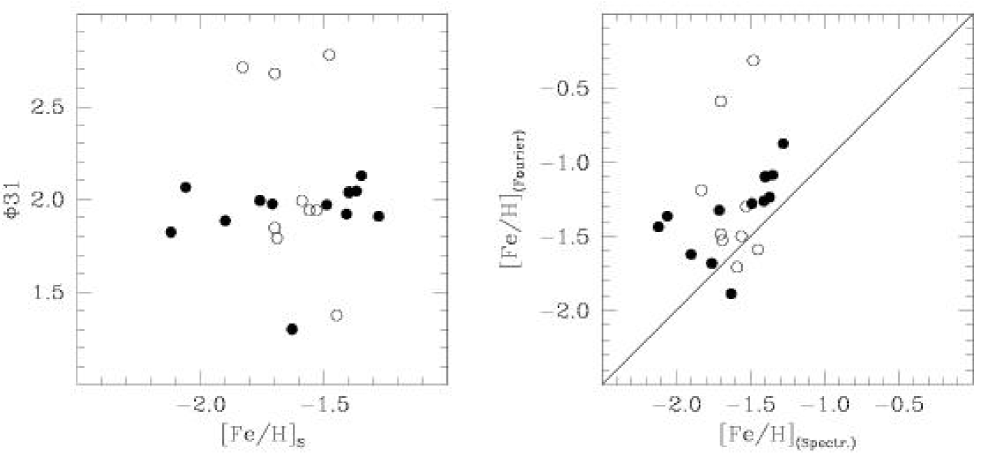
Figure 28: Left panel: run of the $\phi$31 values with the spectroscopic metal abundance for the 22 stars analyzed by G04. Right panel: star-to-star comparison between photometric and G04 spectroscopic metallicities. For ease of comparison we show the 1:1 line. Filled and open symbols and are used for the variables with D${}_{\rm m}\leq 3$ and 3$<$D${}_{\rm m}\leq 5$, respectively.

G04 measured the metallicity for 22 of these stars using low resolution spectroscopy obtained with the VLT. The spectroscopic abundances are listed in column 5 of Table 17. They have average uncertainty of about 0.14 dex and span the metallicity range: $-2.12<$[Fe/H]$<-1.28$, in G04 metallicity scale. This scale is on average 0.2 dex more metal poor than Jurcsik (1995) scale (see G04).

The average difference between photometric and spectroscopic metallicities is 0.30$\pm$0.07 dex, with the photometric abundances being larger as expected. In the left panel of Figure 28 we show the run of the $\phi$31 values with G04 metal abundances, and in the righ panel the star-to-star comparison between photometric and G04 spectroscopic metallicities for these 22 stars.

The correlations in both panels are not very strong, though, admittedly, some of the most deviating objects have large D_m values.

6.2 Absolute magnitudes

M_V values were derived from the Fourier parameters A₁ and A₃ using equation (1) of K02 with the zero point set in agreement with the distance modulus: $\mu_{LMC}$=18.515$\pm$0.085 for the LMC and the dereddened average visual magnitude of the LMC RR Lyrae stars: $<V(RR)>_{0}$=19.064$\pm$0.064 by C03, implying M_V=0.549 at [Fe/H]=$-$1.5. These values are listed in column 6 of Table 17. Errors have been computed from equation A.2 in KW01, with standard deviations of the Fourier parameters A₁ and A₃ taken from Table 2 of KK98. The uncertainties of the M_V values appear surprisingly small. For comparison in column 7 we list the M_V values computed from the observed apparent intensity-averaged magnitudes (taken from column 8 of Tables 5 and 6) dereddened for $E(B-V)$=0.116 and 0.086 in field A and B respectively (C03) and the standard estinction law A_V=3.1$\times E(B-V)$, on the assumption of $\mu_{LMC}$=18.515$\pm$0.085 (C03).

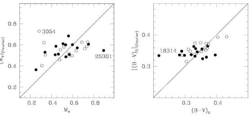
Figure 29: Star-to-star comparison between M_V values (left panel) and $(B-V)_{0}$ colours (right panel) derived from the Fourier parameters of the light curves and the corresponding observed quantities. For ease of comparison we show the 1:1 lines. Filled and open symbols mark variables with D${}_{\rm m}\leq 3$ and 3$<$D${}_{\rm m}\leq 5$, respectively.

The star-to-star comparison between M_V values is shown in the left panel of Figure 29. The reduced range of the (M_V)_Fourier values compared to the observed M_V’s is quite surprising. If we remove the two major outliers (stars # 3054 and 25301) the (M_V)_Fourier values still span only 60% of the range spanned by the observed M_V’s. The larger range of the observed M_V’s can be only partially justified by the actual intrinsic depth of our LMC observed fields (see discussion in Section 3.1 of C03).

6.3 Intrinsic $(B-V)_{0}$ colours and effective temperatures

$(B-V)_{0}$ intrinsic colours were computed from the Fourier parameters A₁ and A₃ using equation (6) of KW01 which is based on the zero points established by KJ97 for magnitude-averaged magnitudes. The values of $\log T_{eff}$ were then computed from these $(B-V)_{0}$ colours using equation (11) of KW01 and adopting $\log g$=2.75 for the average gravity as suggested by several Baade-Wesselink studies. Derived values are listed in columns 9 and 10 of Table 17, respectively. Observed $(B-V)_{0}$ colours were computed from the magnitude-averaged values in column 11 of Tables 5 and 6 and dereddened according to the $E(B-V)$ values in C03, these colours are provided in column 8 of Table 17. The comparison between derived and observed colours is shown in the right panel of Figure 29. As with the absolute magnitudes, the [$(B-V)_{0}$]_Fourier colours cover an interval about 40% smaller than that spanned by the observed $(B-V)_{0}$’s.

In conclusion, the comparison between empirical determinations from the Fourier parameters of the light curves and corresponding observed quantities for the 29 ab-type RR Lyrae stars in the LMC has revealed a number of discrepancies, in particular between the derived and observed M_V and $(B-V)_{0}$ values, deserving deeper investigation based on larger samples of stars than available here. In this respect, we notice that similar discrepancies in the M_V and $(B-V)_{0}$ values have been found by Cacciari et al. (2004), from the analysis of the RR Lyrae stars in M3, and in the M_V values of the variables in $\omega$ Cen (Clement & Rowe 2000) and M15 (Kaluzny et al. 2000).

Appendix A Atlas of the light curves

Atlas of the light curves for the 162 short period variables stars in our two LMC fields. The photometric data are folded with the ephemerides given in Table 5 and 6. Variables stars are divided per field and grouped by type: RR Lyrae stars (ab-, c-, d-type separately), $\delta$ Scuti, candidate Anomalous Cepheids, Cepheids, eclipsing binaries, and within each group are ordered by increasing period.

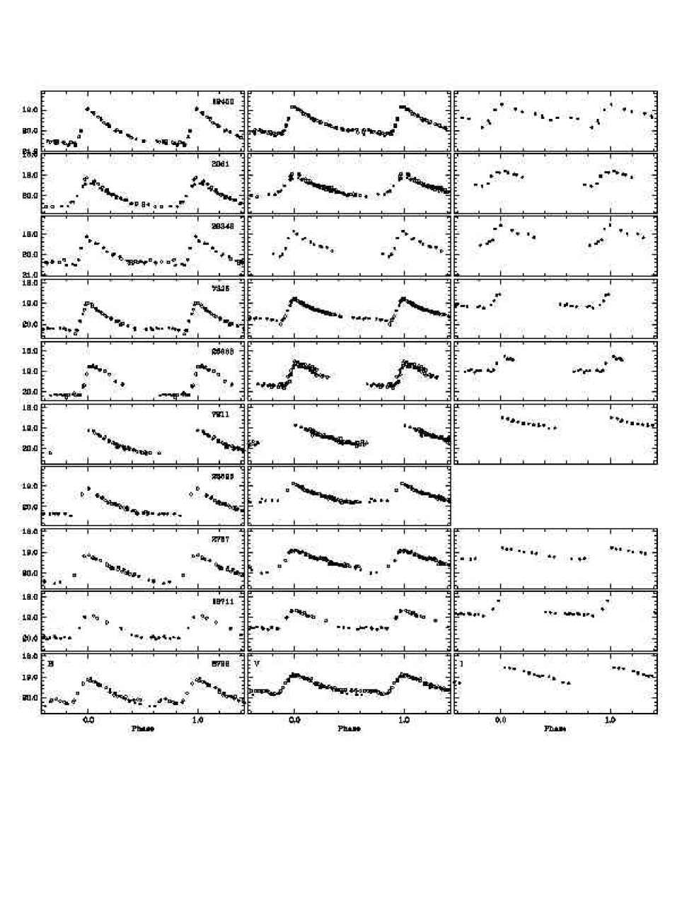
Figure 30: $B,V,I$ light curves of the ab-type RR Lyrae stars in field A, variables are ordered by increasing period. Open and filled symbols are used for the 1999 and 2001 data, respectively.

Fig. A.1. – continued –

Fig. A.1. – continued –

Fig. A.1. – continued –

Fig. A.1. – continued –

Fig. A.1. – continued –

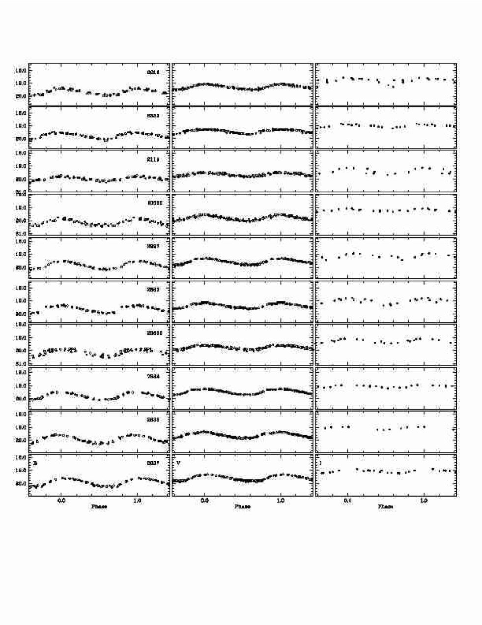
Figure 31: $B,V,I$ light curves of the c-type RR Lyrae stars in field A, variables are ordered by increasing period. Open and filled symbols are used for the 1999 and 2001 data, respectively.

Fig. A.2. – continued –

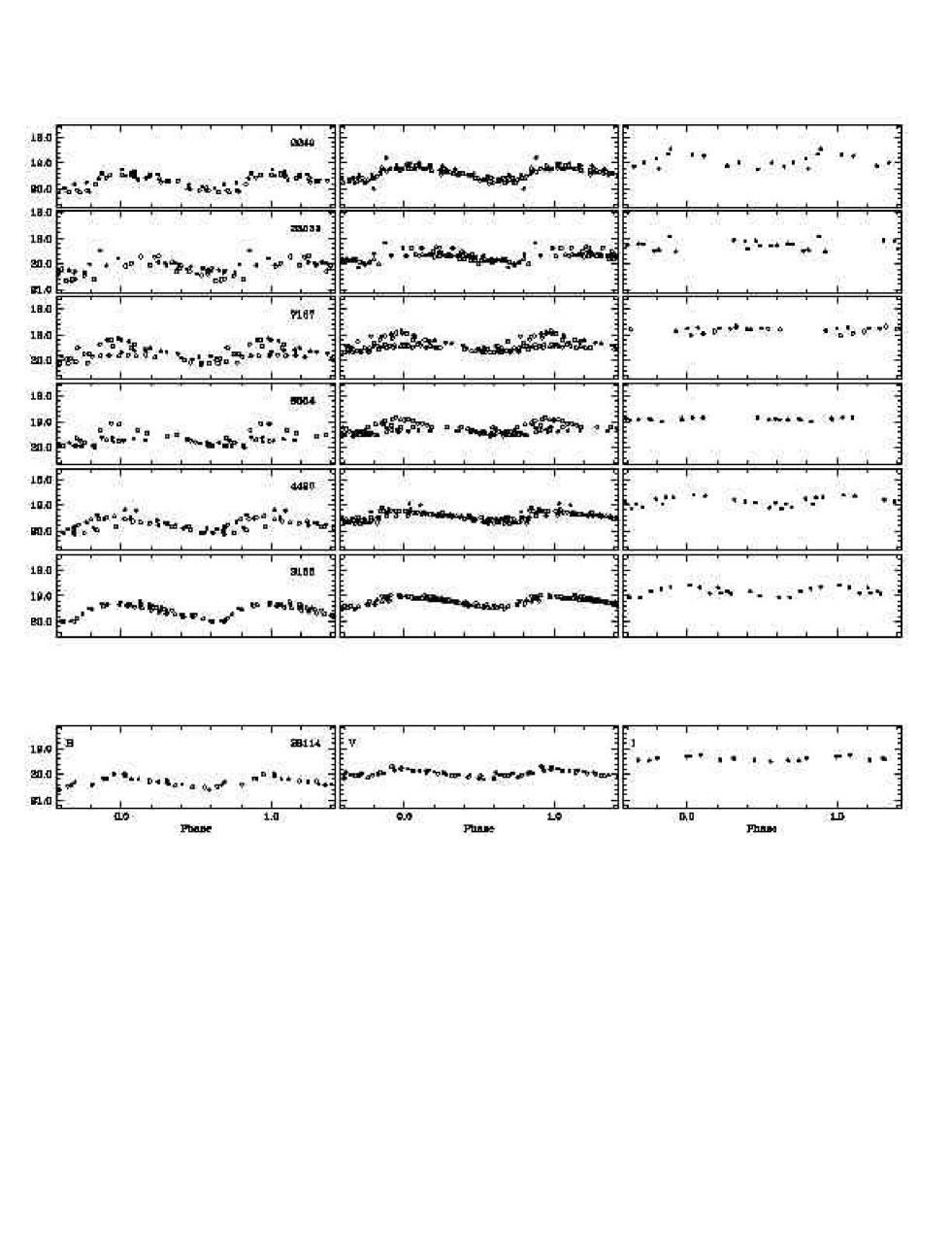
Figure 32: $B,V,I$ light curves of the d-type RR Lyrae stars and of the $\delta$ Scuti star (bottom panel) in field A, variables are ordered by increasing period. Open and filled symbols are used for the the 1999 and 2001 data, respectively.

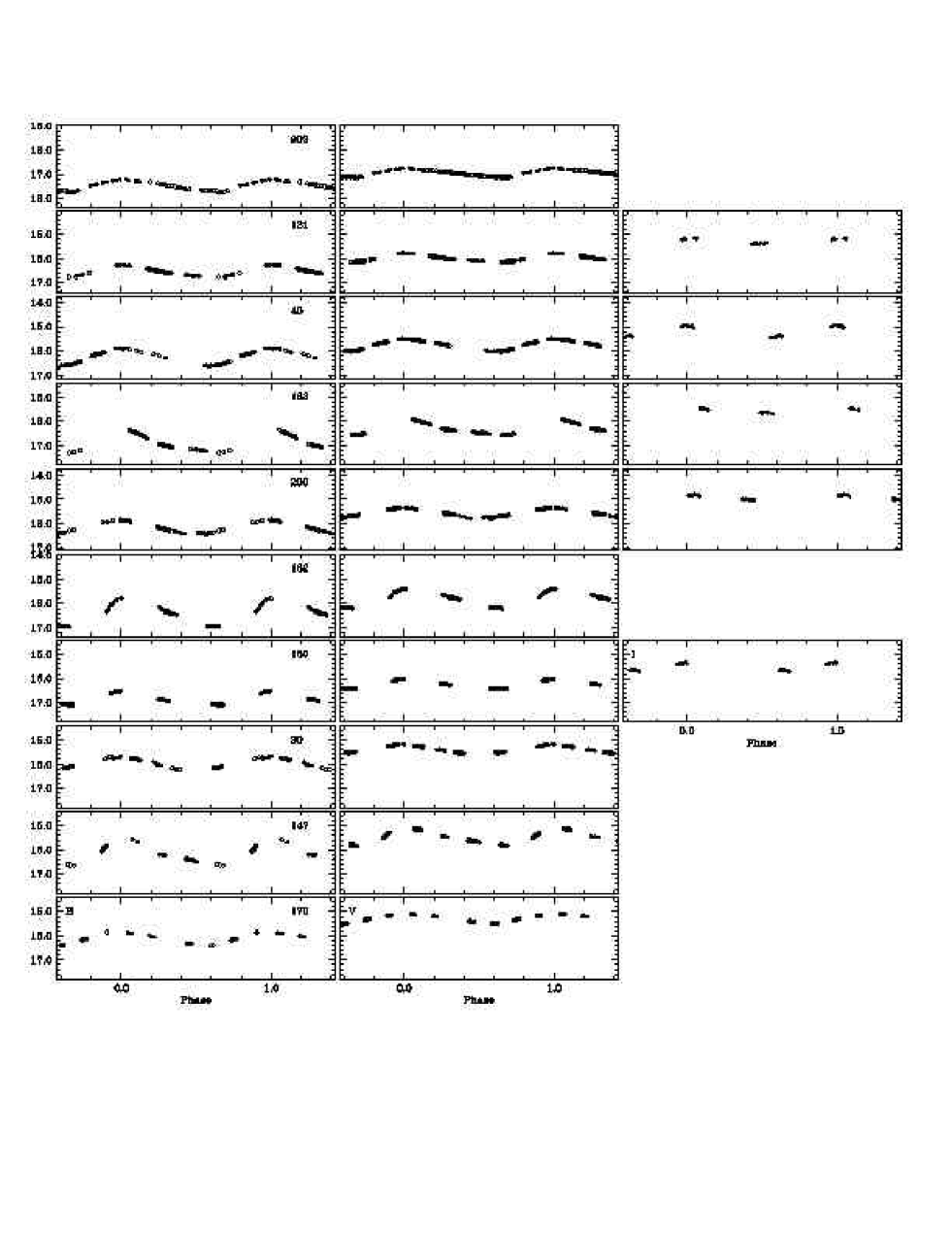
Figure 33: $B,V,I$ light curves of Classical Cepheids in field A, variables are ordered by increasing period. Open and filled symbols are used for the 1999 and 2001 data, respectively.

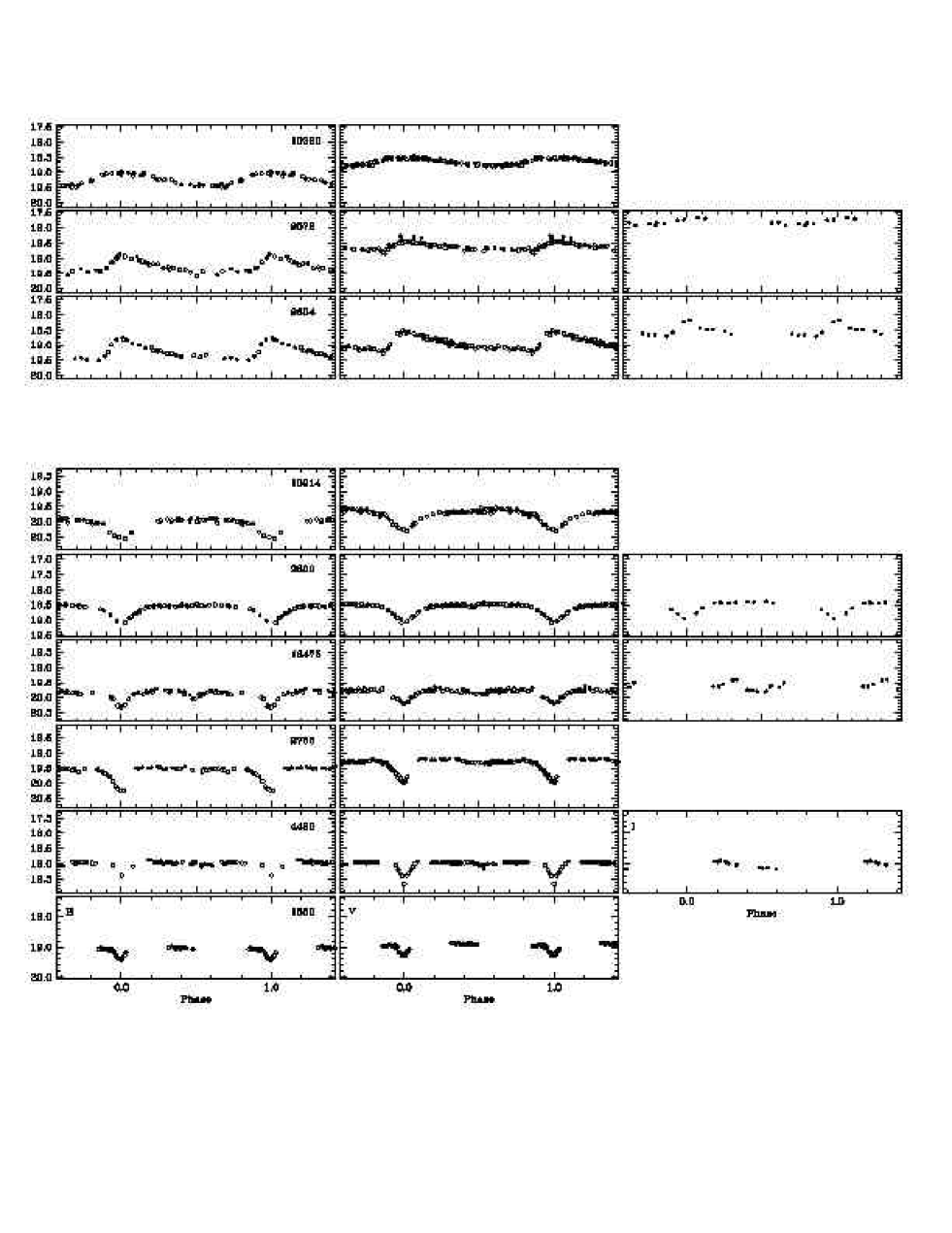
Figure 34: $B,V,I$ light curves of candidate Anomalous Cepheids (first three top panels) and binaries in field A, variables are ordered by increasing period. Open and filled symbols are used for the 1999 and 2001 data, respectively.

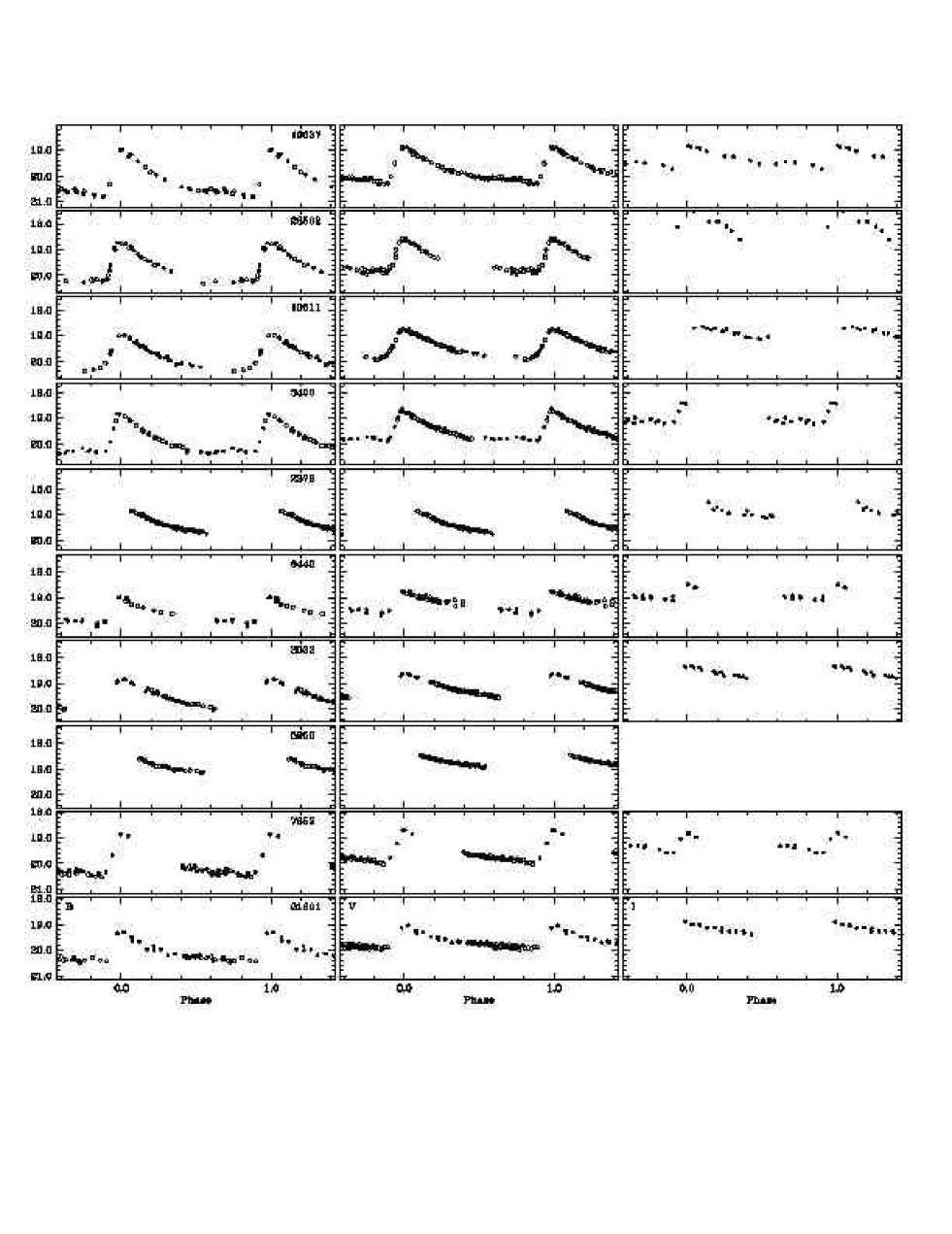
Figure 35: $B,V,I$ light curves of the ab-type RR Lyrae stars in field B, variables are ordered by increasing period. Open and filled symbols are used for the 1999 and 2001 data, respectively.

Fig. A.6. – continued –

Fig. A.6. – continued –

Fig. A.6. – continued –

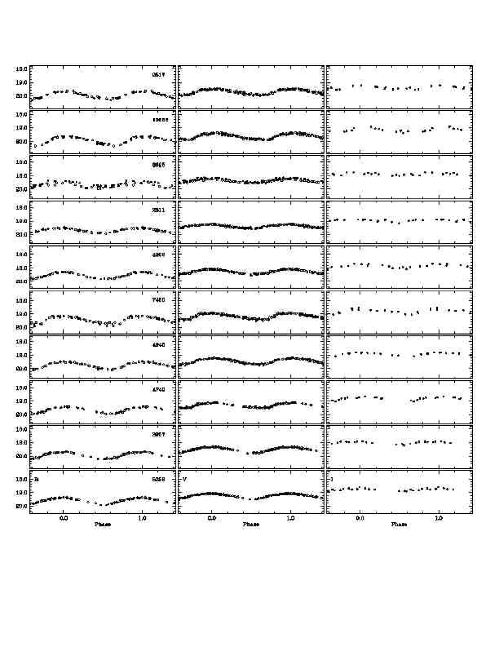
Figure 36: $B,V,I$ light curves of the c-type RR Lyrae stars in field B, variables are ordered by increasing period. Open and filled symbols are used for the 1999 and 2001 data, respectively.

Fig. A.7. – continued –

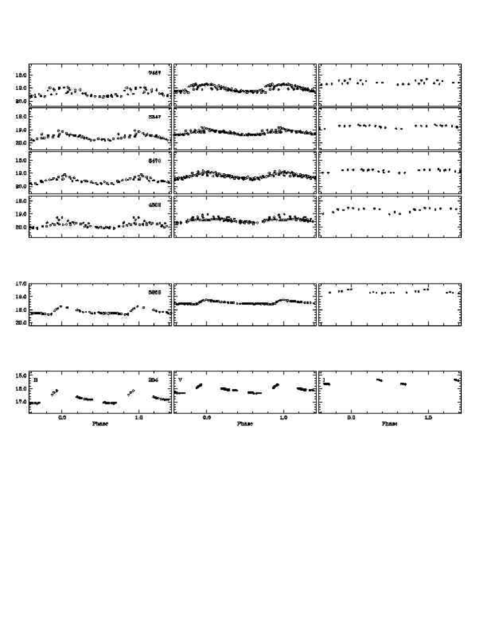
Figure 37: $B,V,I$ light curves of the d-type RR Lyrae stars (first four top panels), Anomalous (fifth panel) and Classical Cepheids (bottom panel) in field B, variables are ordered by increasing period. Open and filled symbols are used for the 1999 and 2001 data, respectively.

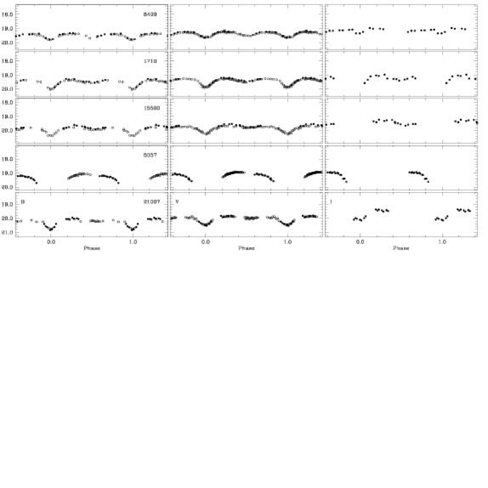
Figure 38: $B,V,I$ light curves of binaries in field B, variables are ordered by increasing period. Open and filled symbols are used for the 1999 and 2001 data, respectively.