Young Super Star Clusters in the Starburst of M82: The Catalogue

Abstract

Recent results from Hubble Space Telescope (HST) have resolved starbursts as collections of compact young stellar clusters. Here we present a photometric catalogue of the young stellar clusters in the nuclear starburst of M82, observed with the HST WFPC2 in H$\alpha$ (F656N) and in four optical broad-band filters. We identify 197 young super stellar clusters. The compactness and high density of the sources led us to develop specific techniques to measure their sizes. Strong extinction lanes divide the starburst into five different zones and we provide a catalogue of young super star clusters for each of these. In the catalogue we include relative coordinates, radii, fluxes, luminosities, masses, equivalent widths, extinctions, and other parameters. Extinction values have been derived from the broad-band images. The radii range between 3 and 9 pc, with a mean value of 5.7 $\pm$ 1.4 pc, and a stellar mass between 10⁴ and 10⁶ $M_{\odot}$. The inferred masses and mean separation, comparable to the size of super star clusters, together with their high volume density, provides strong evidence for the key ingredients postulated by Tenorio-Tagle, Silich, & Muñoz-Tuñón (2003) as required for the development of a supergalactic wind.

1 Introduction

The Hubble Space Telescope has revealed star formation in starburst as collections of centrally condensed super star clusters (SSCs) also referred to as young globular clusters. SSCs are young star clusters with very high luminosity and compactness (Ho, 1997). Their typical sizes (1–6 pc, Meurer, 1995; Maíz-Apellániz, 2001) and masses ($\sim$3 $\times$ 10⁴–10⁶ $M_{\odot}$) are similar to those of globular clusters and they present a typical bolometric luminosity in the range 10⁴⁰–10^42.5 (Strickland & Stevens, 1999). SSCs seem to be protoglobular clusters; they have a large mass and a Salpeter-type initial mass function (IMF), although other possibilities have also been considered (see Kaaret et al., 2004, and references therein). SSCs have been found in interacting galaxies (the Antennae; Whitmore et al., 1999), in starburst galaxies (NGC 253; Watson et al., 1996), and also in star formation regions in normal spiral galaxies (Larsen & Richtler, 1999). For an exhaustive review see the proceedings of the recent meeting The Formation and Evolution of Massive Young Star Clusters, held in November 2003 (to be published by ASP).

M82 provides the best example of a supergalactic wind (SGW) in the local Universe. It has a biconical extended filamentary structure, as evidenced by Subaru (Ohyama et al., 2002), embedded in a pool of soft X-ray emission as detected by Chandra (Griffiths et al., 2000) and XMM–Newton (Stevens et al., 2003) and extending several kpc away from the nuclear region. Moreover, its proximity made M82 a target for a large number of observational programs with HST. The observations now available led us to go into the analysis of the SSC candidates with the aim of measuring the physical properties of a collection of SSCs able to develop and sustain a supergalactic wind.

M82 is nearby and luminous; its H$\alpha$ luminosity is 1.07 $\times$ 10⁴¹ erg s^-1 (Lehnert & Heckman, 1996) after correction for galactic extinction. In this paper a distance of 3.6 Mpc, or m - M = 27.8 mag, is assumed, based on the Cepheid distance to M81 obtained by Freedman et al. (1994). The corresponding linear scale is 1^′′ = 17.5 pc.

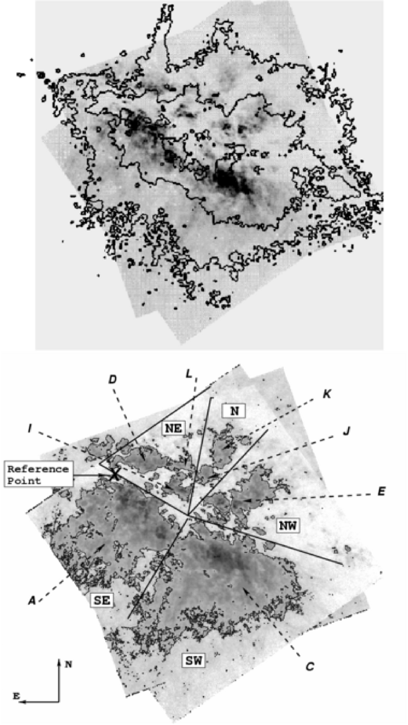
Figure 1: The central region of M82. Upper image: WFPC2 H$\alpha$ image with the NICMOS Fe ii isocontours (Alonso-Herrero et al., 2003) emission superimposed. The lower image shows the zones seen in the WFPC2 H$\alpha$ image used in this paper (the names are indicated in white boxes). The nomenclature propose by O’Connell & Mangano (1978) is indicated outside the image with dashes arrows.

The total extinction in the central regions of M82 is very high and patchy, and is mainly caused by a number of dark lanes crossing it (see Figure 1), which has led to a wide range of extinction values in the literature. For example, O’Connell & Mangano (1978) used an internal extinction of $A_{V}=2.5$ mag but more recent studies (see, e.g., Watson, Stanger & Griffiths, 1984; O’Connell et al., 1995; Satyapal et al., 1995; Alonso-Herrero et al., 2003) give extinction values in the range 2.5 mag $<A_{V}<$ 25 mag.

Although the HST data archive covers the whole central starburst of M82, only the region M82-B (de Grijs, O’Connell & Gallagher, 2001; Parmentier, de Grijs & Gilmore, 2003; de Grijs, Bastian & Lamers, 2003) and the cluster M82-F (Smith & Gallagher, 2001) have been studied in detail. M82-B is also known as the “fossil starburst” of M82 where de Grijs et al. (2001) identified super star cluster candidates after analyzing HST images (WFPC2). de Grijs et al. (2003) also found in this region a peak formation epoch at $\sim$1100 Myr for a sub-sample of clusters with well-determined ages.

In this paper we present a catalogue of young SSCs in the active starburst of M82, the first detailed catalogue of the region, with relative positions and parameters, such as luminosities, compactness and number of super star clusters, relevant to study the evolution of a starburst. In Section 2 we describe the data processing and analysis. Section 3 describes the procedure developed to detect and measure the properties of SSC candidates. Section 4 presents the physical properties of the young clusters, and a discussion of the results is given in Section 5.

2 Data Calibration and Analysis of HST/WFPC2 Images

The data were retrieved from the Hubble Space Telescope public data archives and correspond to three different observational programs (see Table 1). In this paper we analyze the H$\alpha$ (F656N) images. Nitrogen ii images ([N ii] $\lambda$6583.6 Å—F658N) are used to eliminate the contribution of this line in the H$\alpha$ images. Some broad-band images (F547M—$Str\ddot{o}mgren$ $\it y$ and F814W—I filter) are used to eliminate the contribution from the background continuum. On the other hand, all broad-band images are used to calculate the extinction and masses of SSCs (section 3.4). Images are retrieved already processed by the standard WFPC2 pipeline. The calibration factor is obtained with the STSDAS package synphot. Each field is observed in four exposures, which allows us to combine them to eliminate cosmic rays (the crrej task in the stsdas package). The calibration precision of the photometry is better than 5 $\%$ (Biretta et al., 2002).

The WFPC2 comprises four 800 $\times$ 800 pixel cameras. Three of these (the Wide Field chips or WF) have a scale of 0.1^′′/pixel and the fourth (the Planetary Camera or PC) has a scale of 0.046^′′/pixel. For more information see Biretta et al. (2002). We have used the PC images whose fields entirely cover the starburst area of M82 in all filters but F814W, F439W and F555W; these are covered by the WF4 camera. In order to match the PC pixel size, the F814W image has been oversampled. The geometric distortion was corrected using the drizzle task.

The next step in the data processing is to subtract the continuum contribution from the H$\alpha$ emission. Ideally, one would use one or two narrow-band filters adjacent in wavelength to H$\alpha$ to estimate the continuum. In practice, such filters are usually not available and one has to use either (a) a wide-band filter close in wavelength but contaminated by emission lines or (b) two encompassing filters at a certain distance in wavelength, from where one can interpolate the continuum at H$\alpha$. Here, we follow the second approach since there is no $R$ band image available in the archive. For the continuum at wavelengths longer than H$\alpha$ there is only one filter available, F814W. In the blueward side, we can choose between F555W and F547M. F555W is wider and provides a better S/N but it has one severe problem: it is contaminated by [O III] $\lambda$4959+5007 and, to a lesser degree, by H$\alpha$ itself and H$\beta$. For that reason we selected F547M as our blueward filter. We interpolated in wavelength the spectrum between F547M and F814W choosing a synthetic spectra of synphot (White et al., 1998) in IRAF (Tody, 1986) for an atmosphere of a star with $T=30\,000$ K (Kurucz, 1979) whose ($F547M-F814W$) color matches the one measured. Finally, we selected the value of the spectrum at the wavelength of H$\alpha$ to estimate the continuum contribution to F656N.

We also estimated the charge transfer efficiency corrections ($\pm$1 percent) and considered these not to be necessary. Finally, the images were rotated to set them at the standard orientation (north up and east left).

After calibration and continuum subtraction of the WFPC2 data, we compared our results with previous work. O’Connell & Mangano (1978) measured the H$\alpha$ luminosity in all of M82-A and corrected for reddening (A_V = 2.5), they obtained a luminosity of 5.06 $\times$ 10⁴⁰erg s^-1 (the difference in distance has been allowed for). Correcting for the same reddening and inside a contour of 3 $\times$ 10^-17 erg s^-1 cm${-2}$, we measured 5.02 $\times$ 10⁴⁰ erg s^-1, confirming the WFPC2 data calibration.

3 Detection and Measurement of Candidate SSCs

The starburst of M82 is crossed by dark lanes which divide it into five different zones (see Figure 1, lower image), here used as reference to locate the SSCs in the nucleus of M82. The figure (top panel) also shows the HST/WFPC2 image overlaid with isocontours of the HST/NICMOS [Fe ii]1.644 $\mu$m image (Alonso-Herrero et al., 2003). As the [Fe ii] emission is not as affected by extinction, it allows a deeper view into the otherwise dark lanes in the visible, and this reveals the starburst as a continuous extended region. Note also how the [Fe ii] emission follows the structure of the filaments seen in the visible, particularly in the northern part.

The correspondence between the five zones (named in Figure 1, lower panel) and the O’Connell & Mangano (1978) sequence of bright regions in M82, extended as to also include the smaller regions (I - L) is given below:

N

: zone to the north (J+K)

NE

: zone to the northeast (I+D+L)

NW

: zone to the northwest (E)

SE

: zone to the southeast (A)

SW

: zone to the southwest (C)

Note that region B, or the fossil starburst of M82 (de Grijs et al., 2001), is to the east of the starburst and outside the PC field.

The zones evidently host a plethora of compact knots, with a variety of sizes. However, not all bright H$\alpha$ knots can be associated with SSCs. They may result from H ii regions ionized by an embedded young super star cluster, or could also be dense clouds illuminated from the outside by nearby clusters. The inhomogeneous extinction is also important, since it limits the number of observed SSCs in a manner difficult to estimate.

To discriminate among the various possibilities, three independent analyses of the images were carried out. First we consider the error values in equivalent width, second we look for holes in the extinction map, and third we thoroughly analyze the continuum image. We identified bright knots both in H$\alpha$ and continuum images and selected as young super star cluster candidates, those which are detected in both images. Knots that only emit in H$\alpha$ are most probably illuminated clouds, whereas those that only show up in the continuum were declared old clusters; neither of these types are included in the catalogue.

3.1 Search for bright knots

Bright knots were selected using daofind (Stetson, 1987), as implemented in IRAF and using a feature detection threshold of 15-sigma. daofind was optimized for the identification of pointlike sources, (roundish structures), what led us to consider it as suitable for finding compact SSCs. However, few of them ($\leq$ 3%), not being circular enough, are missed by the software. The “amorphous” SSCs are either more than one SSC superposed in projection or clusters suffering channeled outflows of ionized material. All the SSCs with emission outside the roundish structures were followed and marked with an asterisk in the catalogue to indicate the cases where a lower limit to the measured flux is given.

Specific software was developed to identify and measure SSC candidates in nearby galaxies using ground-based observations (Larsen, 1999). However, the case we are analyzing is different. The problem is not PSF and seeing deconvolution but crowding, and to define an algorithm able to identify and measure a high density of sources such as those present in M82 and other starbursts. To ascertain the radii of SSCs is not an easy task because of crowding in some areas; there are many SSCs in a very small region so their fluxes are mixed. The procedure we have designed is as follows. From the already identified maxima, we made concentric apertures of increasing radius ($\Delta r$ = 1 pixel), from 1 to 10 pixels, using the phot task in apphot (IRAF) (equivalent to 0.81–8.05 pc) and compute the flux profile for concentric annuli at different radii both for H$\alpha$ and for the continuum. We fit the resulting flux distribution of each knot with a third-order polynomial and calculate the inflection points. In this way we establish the size and the overlap limit with the nearest neighbors. For the case of clusters with very close companions, the estimated radius is a lower limit that clearly depends on the crowding in this region. In Figure 2 two different cases are shown. The upper graph is a difficult case because the profile is very monotonic due to crowding. The lower curve represents an isolated SSC where it is relatively easy to find the limit of the region. The method works properly in most cases. Tables 3 and 4 (see also section 4) list the emission peak centers and the estimated angular sizes, from both H$\alpha$ and the continuum images, respectively. The complete tables are on-line in the electronic version of this paper. In most cases (72%) the separation ($\Delta$ in pc) between neighboring knots is larger than the sum of their radii and thus our method provides in such cases size values down to the background level. The remaining 28% are marked with a $\ddagger$ in Tables 5–9.

3.2 Final sample

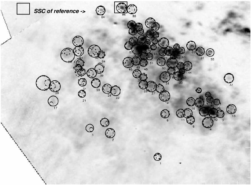
Figure 3: Final sample of young SSCs within the SE zone. Young SSC radii are overplotted on the image: the dashed lines are H$\alpha$ knots, the dash-dotted lines are continuum knots, and the solid lines are the final radii including both types of emission. The SSC used as a reference point is indicated within a box. (See the electronic edition of the Journal for a color version of this figure.)

We compiled a catalogue of the bright knots in H$\alpha$, and in the continuum images. Then, from both listings we take only those that emit both in H$\alpha$ and the continuum and that overlap by at least half the diameter of the smaller determined areas. The final associated SSC radii (solid lines in Figure 3) account for the overlap between the estimated size of the H$\alpha$ (dashed line in Figure 3) and of the continuum emission (dash-dotted line in Figure 3). When one of the apertures (H$\alpha$ or continuum) includes the other, we take the larger one. In all other cases, a new aperture engulfing the other two is defined and used as the radius of the corresponding SSCs.

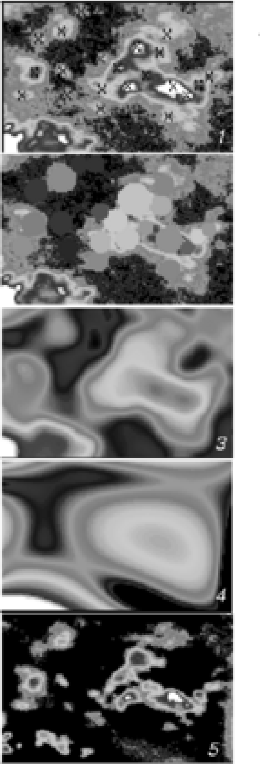
Figure 4: The method. Sequence of steps followed to model and subtract the diffuse emission in region M82-I. 1: H$\alpha$ image with young SSCs marked; 2: H$\alpha$ image with overlapping masks in it (see text for further explanation); 3: map 2 is smoothed with a Gaussian; 4: map 3 is fitted with a spline function in two dimensions; 5: H$\alpha$ image without diffuse emission. (See the electronic edition of the Journal for a color version of this figure.)

We have subtracted the underlying diffuse emission of the galaxy and present in the catalogue the total fluxes as well as fluxes without the diffuse emission contribution. Figure 4 shows, as an example, the sequence of steps followed to model the diffuse emission map for region M82-I. The first step is to create masks in the H$\alpha$ map on each SSC position, of the same size as the radius of the SSC and with a value equal to the average flux found within the following annulus (1 pixel wide) after that radius (step 2 in Figure 4). We then smooth this mask-map with a Gaussian, the width of which is equal to the average radius for each region (Figure 4, step 3). A model of the diffuse emission using a larger gaussian leads to border effects around the SSCs. After testing several other possibilities we finally adjusted the smoothed map with two dimensional spline functions (FIT-REGION, IDL, Molowny-Horas & Yi, 1994). The best adjustments are with a fourth-order function (Figure 4, step 4). The adjusted map is the diffuse emission map to be subtracted from the H$\alpha$ map in order to have a measure of the SSC fluxes without this contribution. Naturally, the procedure will only select as a SSC candidate those knots with a H$\alpha$ emission larger, in each aperture, than its local diffuse emission as derived from the diffuse emission map.

We also adjusted the diffuse emission map of the continuum image to estimate the H$\alpha$ equivalent width ($W({\rm H}\alpha)$) without the diffuse emission contribution. We obtained the $W({\rm H}\alpha)$ of the H$\alpha$ emission line as the ratio of the H$\alpha$ emission line flux to the continuum flux, both without the diffuse emission contribution, within the final catalogued aperture of each young SSC.

3.3 Comparison with FOCAS

We used the FOCAS package in IRAF for comparison. FOCAS is basically used for automatic detection, photometry, and cataloguing of H ii regions, using masks with the areas of the structures found. As in all methods, the problems start in crowded regions when the flux from neighboring bright knots begins to overlap.

Table 2 compares the fluxes measured with FOCAS and with our method in region M82-I. Fluxes and areas measured with our method are larger than those measured with FOCAS. The most important reason is that in most regions there are large differences in the determined object positions between the two methods. The differences arise because FOCAS takes the geometrical center of regions and our method looks for the brightest point. FOCAS is able to find a region with almost any shape, while our method assumes SSCs to be compact, centrally concentrated round clusters and avoids contamination with other H$\alpha$ emission possibly associated with them.

3.4 Extinction, ages and masses

As previously mentioned, the central regions of M82 experience a strong and variable extinction, hence each of the clusters in our sample requires an individualized extinction measurement. In order to calculate it, we extracted the F814W, F555W, F547M and F439W fluxes for each cluster using an aperture-photometry program written in IDL and we applied to them the aperture correction (Holtzman, J. et al., 1995). The program was run using the original images (unrotated and without drizzling) to minimize flux calibration effects. In order to measure the extinction from the continuum colors, we used FITMODEL (Maíz-Apellániz, 2004), a $\chi^{2}$-minimization code that searches through the parameter space for multiple solutions and provides uncertainty estimates with possible pre-established constraints. We inputted the WFPC2 photometry for all the clusters in our sample into FITMODEL using as a comparison Starburst99 SEDs (Leitherer et al., 1999) of ages between $10^{6}$ and $10^{10}$ years, with solar metallicity, and extinguished using a Cardelli et al. (1989) law with $R_{5495}=3.1$. FITMODEL generates a likelihood plot as a function of the chosen parameters, in our case age and $E(4405-5495)$, that can be used to derive the expected values and their uncertainties. Unfortunately, the derivation of ages and extinction of stellar clusters using broad-band optical photometry is hampered by the existence of color degeneracies for the parameters one is trying to measure (Anders et al., 2004b). Therefore, for many clusters the reddening values derived in this way are of little use due to their large uncertainties unless some additional information about the age is included.

Ages can be estimated independently using the equivalent widths of the Balmer lines. During the first 6 Myr of the life of a cluster formed in an instantaneous burst of star formation, the existent O and WR stars generate large numbers of ionizing photons which produce large equivalent widths of the Balmer emission lines (for solar metallicity and H$\alpha$, $W({\rm H}\alpha)$ larger than 100 Å). At an age of $\approx$ 6 Myr, the last of the single O stars explodes as a SN and the ionizing flux of the cluster would drop to very low values if it was not for O stars produced in binaries by mass transfer (Cerviño & Mas-Hesse, 1999; van Bever et al., 1999). Those stars “rejuvenate” the cluster and maintain values of the $W({\rm H}\alpha)$ between 10 and 100 Å until the cluster is $\sim$ 25 Myr old. Unfortunately, a number of factors such as photon leakage, presence of an underlying stellar population, differential extinction, and stochastic fluctuations in the IMF (see, e.g Maíz-Apellániz et al., 1998; Cerviño et al., 2003) hamper the derivation of exact ages from the equivalent widths of the Balmer lines for unresolved or slightly resolved young clusters. Despite that caveat, for solar metallicities it is quite safe to give an age between 1 and 6 Myr for a cluster with $W({\rm H}\alpha)>100$ Å and an age between 6 and 25 Myr for a cluster with $100$ Å $>W({\rm H}\alpha)>10$ Å. For the case of M82, the only circumstance that is likely to invalidate the above criterion for age estimation would be the existence of two clusters, one young and one old, along the same line of sight.

With the age constraints derived from the $W({\rm H}\alpha)$, we obtained the expected values and uncertainties for the extinction of each cluster. Results are shown in Tables 5–9 (column 9). In a few cases, the FITMODEL output indicated that the likelihood of the age ranges determined from the $W({\rm H}\alpha)$ was significantly lower than that of older ages, likely due to superposition between two clusters of different ages. Those cases should be considered to be more uncertain than the rest and are marked in Tables 5–9 by a $\dagger$ symbol.

The extinction values obtained in this study are in agreement with the contour map extinction presented by Waller et al. (1992).

Stellar masses have been estimated from broad-band magnitudes (stellar continuum) taking into account the age and $W({\rm H}\alpha)$ constraints explained in the previous paragraphs and using the following expression:

$$2.5~{}\log(\frac{M}{M_{\odot}})~{}=~{}M_{V,1}(0)+(5~{}\log(d)~{}-~{}5)-(m_{V}~{}-~{}A_{V}~{}-~{}C(t))$$ (1)

where:
- M = cluster mass
- M_V,1(0) = absolute V magnitude of a cluster normalized to one solar mass for zero age (obtained from Starburst99)
- (5 log(d) - 5) = distance modulus
- m_V = apparent V magnitude
- A_V = extinction coefficient in V
- C(t) = age correction = M_V,1(t) - M_V,1(0)

For comparison, masses for SSCs with $W(H\alpha)$ larger than 100 Å have also been estimated using Starburst99 (Leitherer et al., 1999) and the $W(H\alpha)$ under the assumption of coeval bursts. The agreement is excellent; with Starburst99 and using the $W(H\alpha)$ a mean value of 1.97 $\times$ 10⁵ M_⊙ with a standard deviation of 1.80 $\times$ 10⁵ M_⊙ is obtained. Following the procedure explained above, a mean mass of 1.75 $\times$ 10⁵ M_⊙ with a standard deviation of 2.05 $\times$ 10⁵ M_⊙ is obtained. In Tables 5–9 (column 14) we present the stellar masses estimated from broad-band photometry.

4 The Catalogue

In this section we present the resulting catalogue of SSCs in the nuclear region of M82. In the first set of tables we list the positions and radii of the brightest knots found in the H$\alpha$ (Table 3) and the continuum (Table 4) images, sorted by declination in each zone. In these tables we present only the first ten knots, the full lists may be acquired from the electronic version of the paper. The typical residual pointing error in WFPC2 images is 0.86^′′, $1.84^{\prime\prime}$ being the largest error seen (Biretta et al., 2002, chap. 7), it is thus necessary to find a point of reference in the image. We could not obtain the absolute astrometry for the clusters due to the absence of either USNO2 (Monet et al., 1998) or Tycho-2 (Høg et al., 2000) in the field of view of these images. We use u3jv0201r and u3jv0202r images as reference. The coordinates of knots and young SSCs are relative to the coordinates of one young SSC located within the SE zone (number 86 in Table 5). This one is marked in Figure 3 and its coordinates are: RA = 9^h 55^m 53.56^s and Dec.= 69^∘ 40^′ 51.78^′′. We have checked that this young SSC emits in all the filters we have used and also in the near infrared bands, e.g. in Alonso-Herrero et al. (2003) and McCrady, Gilbert & Graham (2003) who also report this knot (MGG-1a), so we consider it a good reference point. We have compared our coordinates with those provided by McCrady et al. (2003) who had adjusted their astrometry to match with the positions listed in Kronberg, Pritchet & van den Bergh (1972). The agreement with MGG-1a (McCrady et al., 2003) is good (a difference of 2” in declination).

Tables 5–9 list the final sample of SSCs in each zone sorted by declination. Column 1 gives the identification number of young SSCs candidates. SSCs with emission outside the roundish structures are marked with an asterisk. This additional emission is either more than one SSC superposed in projection or clusters suffering channeled outflows of ionized material. SSCs which have problems with their age determination are marked with a $\dagger$ symbol. Columns 2 and 3 list the R.A. offset (seconds) and the Dec. offset (arc seconds) with respect to the reference SSC; column 4 gives the radius (pc); column 5 gives the H$\alpha$ flux (10^-15 erg s^-1 cm^-2); column 6 gives the estimated H$\alpha$ diffuse emission flux in each SSC aperture (10^-15 erg s^-1 cm^-2); column 7 lists the H$\alpha$ diffuse emission flux as a percentage of the H$\alpha$ flux (%); column 8 gives the H$\alpha$ flux without diffuse emission (10^-15 erg s^-1 cm^-2); column 9 lists the internal extinction (in V magnitudes); column 10 gives the H$\alpha$ luminosity of the SSCs corrected for galactic and internal extinction and without the diffuse emission contribution (10³⁸ erg s^-1); column 11 gives the projected separation to the nearest SSC ($\Delta$, pc); column 12 lists the number of ionizing photons (10⁴⁹ s^-1) obtained by using the expression given by Osterbrock (1989); column 13 lists the H$\alpha$ equivalent width (Å); and column 14 gives the stellar mass (10⁵ $M_{\odot}$).

As mentioned in section 2, photometric errors are very small, less than 5$\%$. The most important source of error in the flux determination is the aperture selection. We have estimated this error by measuring the flux in the two adjacent apertures to the one that defines the radius (see column 4). The mean value of their difference is taken as the flux error (columns 5, 6 and 8).

Table 10 summarizes the densities of young SSCs, mean values and standard deviation for stellar masses, luminosities, radii and projected separation to the closest SSC for each of the five zones that compose the nucleus of M82. In Table LABEL:tab11 star formation rate values for the different zones analyzed are given. The number of SSCs for each zone is also provided (column 2) as well as the number of them in the two considered age ranges, 1-6 Myr and 6-25 Myr. The star formation rate has been estimated in two ways: using the masses provided in Tables 5–9 and from the total H$\alpha$ luminosity measured on each zone. SFR ($M_{\odot}$ yr^-1) for SSCs with 1-6 Myr and 6-25 Myr respectively and estimated from the mass values provided in Tables 5–9 are given in columns 3 and 4. Columns 5, 6 and 7 give the total H$\alpha$ luminosity (10⁴⁰ erg s^-1) for each zone, and the derived values of SFR and SFR per unit area ($kpc^{2}$). Note that the values provided for the SFR on each zone, using masses estimated with FITMODEL for younger and older SSCs and H$\alpha$ luminosity (columns 3, 4 and 6) are in good agreement.

5 Discussion

The main features of the nuclear clusters catalogued in M82 are their youth, their compactness (5.7 $\pm$ 1.4 pc radii), their high luminosity and, therefore, masses and the SSCs surface density (richness). We found 197 young SSCs in the nuclear starburst of M82 and more may be hidden behind the dark lanes and may have similar properties to those of the SSCs that we have found. Lipscy & Plavchan (2004) found seven star-forming clusters in the mid infrared but neither of them seem to match with the SSCs here found. Using radio images they proved that the mid-IR sources are heavily obscured H ii regions so these mid-IR SSCs may be hidden in the H$\alpha$ images.

Statistics in the SSC parameters for every analyzed zone (5 in total) are given in Table 10. The analysis is summarized in the histograms shown in Figure 5.

SSCs are very compact objects; for example, Meurer (1995) found analysing UV images that the typical FWHM of SSCs in a sample of galaxies is 2.6 pc. The WFPC2 images of M82 in H$\alpha$ had been analyzed by O’Connell et al. (1995), who found a typical FWHM of 3.5 pc for SSCs. Here we have developed a method to estimate the physical size of SSCs that takes into account the H$\alpha$ emission, the emission in the continuum and their overlap. The latter leads to larger size values than other methods where radii are obtained from lower spatial resolution images in only one filter (V, from the WF camera). Figure 5 (top-left) shows a histogram with the size distribution of SSCs in M82. Radii are in the range 3–9 pc with a mean value of 5.7 $\pm$ 1.4 pc (Table 10). Note however, that our values are very similar to those found by Billett et al. (2002) for SSCs in nearby dwarf irregular galaxies and also similar to the values inferred for SSCs in M82-F (Smith & Gallagher, 2001) who found a half-light radius of 2.8 $\pm$ 0.3 pc $\sim$ 1/2 FWHM. Both of the latter studies based on HST/WFPC2 images.

The projected separation to the closest neighbors for each of the young SSC is smaller than 30 pc (see Figure 5–top-right), with a minimum value of 5 pc and a mean separation of 12.2 $\pm$ 7.2 pc (Table 10). The projected typical separation between SSCs (see Tables 5–9) is factors of two to three times larger than the typical size associated to them.

The global density of young SSCs, or number of young SSCs per unit area, is very high in the starburst of M82 (see Table 10). O’Connell et al. (1995) reported about 50 individual luminous clusters in M82-A; this region is equivalent to our SE zone, where we have catalogued 86 SSCs. Zone SE extends over a square area of 242 $\times$ 242 pc² and therefore has a young SSC density of 1468 kpc^-2. For the whole starburst of M82, we estimate a SSC density of 620 kpc^-2. If one compares with other nearby nuclear starburst, like NGC 253, the SSCs density of M82 is much larger. NGC 253 has only four SSCs in its nuclear zone, within an area of 197 $\times$ 180 pc (Watson et al., 1996) and thus a SCC density of 113 kpc^-2, 5.5 times smaller than M82. The differences become larger if the comparison is made with zones NE, N and SE where the highest SSCs density is found in M82.

The SSCs in the nuclear starburst of M82 also show a high H$\alpha$ luminosity (see Figure 5–bottom-left). H$\alpha$ luminosities, corrected for galactic and internal extinction, and without the diffuse emission contribution are in the range 0.01–23 $\times$ 10³⁸ erg s^-1 with a mean value at 3.2 $\times$ 10³⁸ erg s^-1 (Table 10) for all young SSCs in the starburst of M82. If we add together all the SSCs we obtain a total H$\alpha$ luminosity of 6.3 $\times$ 10⁴⁰ erg s^-1.

The stellar masses of SSCs in M82 have been determined using Starburst99 and FITMODEL and our results are displayed in Figure 5 (bottom right-hand panel). The young SSC mass in M82 ranges from 4 $\leq$ $log(M_{\rm SSC}/M_{\odot})$ $\leq$ 6 with a mean value of 1.7 $\pm$ 2.0 $\times$ 10⁵ $M_{\odot}$ (see Table 10). The measured stellar masses highly depend on the applied extinction correction. However, the most massive clusters in M82, have masses similar to those in M82-F, spectroscopically confirmed by Smith & Gallagher (2001). They are also similar to mass estimates for clusters in NGC 1569 (Anders et al., 2004a) that range between 5.7 $\leq$ log(M${}_{\rm SSC}/M_{\odot}$) $\leq$ 6.2. On the other hand, de Grijs et al. (2003) found even more massive clusters in NGC 6745 reaching values up to 10⁸ $M_{\odot}$, although given the distance to this source, compact SSC may be spatially unresolved. McCrady et al. (2003) measured kinematic masses of two of the IR brightest clusters in M82, using high-resolution IR spectroscopy. Only one of them emits in H$\alpha$, MGG-11, which corresponds to our cluster number 5 in the NW zone. Their measured kinematic mass is 3.5 $\times$ 10⁵ $M_{\odot}$, which, considering the difference in the methods, compares rather well with our determination of 4.1 $\times$ 10⁵ $M_{\odot}$.

The star formation rate for the different zones is in the range (0.03–0.8) $M_{\odot}$ yr^-1 (Table LABEL:tab11). The numbers are consistent after obtaining the SFR separately for younger (1-6 Myr) and older clusters (6-25 Myr). The agreement is also very good with the values of the SFR for each zone obtained using the total H$\alpha$ luminosity (column 5, 6 in Table LABEL:tab11). The star formation rate per unit area, $\Sigma_{\rm SFR}$ (see column 7, Table LABEL:tab11) is very large in the five different zones. Our values, ranging between 500-4100, are in agreement with values reported for starbursts by (Kennicutt, 1998, see his Figure 6). Comparing the values for the different zones, the lowest value corresponds to zone N. Although the SSC density is very high in this zone, the mean luminosity of the SSCs is the lowest (see Table 10). Kennicutt (1998) presented also the case of 30 Doradus, which, in its inner 10 pc, has $\Sigma_{\rm SFR}$ $\sim$ 100 $M_{\odot}$ yr^-1 kpc^-2, but the mean $\Sigma_{\rm SFR}$ over the entire H ii region is $\sim$ 1–10 M_⊙ yr^-1 kpc^-2. M82 in thus a case of exacerbated star formation well above the average in the local Universe.

Also important is the spatial distribution of the SSCs in M82. As mentioned before, the largest SSC density (see Table 10) is clearly the eastern one (within the zones labeled NE, N, and SE), which are right at the base of the supergalactic wind filamentary structure. In this respect, as pointed out by Tenorio-Tagle et al. (2003), the interaction of the winds from neighboring SSCs is most probably the key ingredient in the development of a large scale filamentary structure embedded in a pool of X-ray emitting gas as observed in M82. Here, we have identified relevant observational parameters in the study of SGWs, such as the density of SSCs and the comparison between their typical sizes and projected separation. From the catalogue we find that the mean radii of the catalogued clusters is similar to the mean distance among them, which seems to be a necessary condition for the individual winds to interact and generate the oblique shock waves able to channel the material along, straight structures such as the filaments seen in M82.

More detailed analysis of the cluster distribution and the base of the super wind structure will be the subject of a forthcoming paper. There we will use NIR data to identify any possible SSCs completely hidden from view in the optical data and to improve our extinction and age measurements.

Table 1: Log of HST data archive observations

Filter	P.I.	Band	Images	Exposure times (s)
F656N	W. Sparks	H$\alpha$	u2s04201t–2t	2 $\times$ 300
F656N	P. Shopbell	H$\alpha$	u3jv0101r–102r–201r–202r	4 $\times$ 500
F658N		N ii	u3jv0103r–104r–203r–204r	4 $\times$ 600
F547M		Str. ya	u3jv0207r–8r	2 $\times$ 50
F814W	R. O’Connell	WFPC2 I	u45t0105r–6r–7r–8r	2 $\times$ 200/1200/600
			–hr–ir–jr–kr	260/140/2 $\times$ 900
F439W		WFPC2 B	u45t0109r–ar–br–cr	2 $\times$ 400/1000/2300
			–lr–mr–nr–or	500/300/2500/1100
F555W		WFPC2 V	u45t0101r–2r–3r–4m	2 $\times$ 350/1600/800
			–dr–er–fr–gr	300/200/2 $\times$ 1000

Table 2: Comparison between results obtained with FOCAS and our method for the region M82-I.

Id.	$R$a	$F_{\rm H_{\alpha},us}^{b}$	$F_{\rm H_{\alpha},fo}^{b}$	$F_{\rm us}/F_{\rm fo}$	$A_{\rm us}/A_{\rm fo}^{c}$	$\delta$d
1	5.64	4.88	3.76	1.30	1.59	3.2
2	5.64	2.84	1.28	2.22	1.68	1.8
3	5.64	7.13	4.94	1.44	1.43	1.8
4	4.03	16.33	2.35	6.96	8.75	2.6
5	5.64	9.59	1.31	7.34	7.33	1.7
6	6.44	29.47	22.85	1.29	1.59	2.0
7	7.25	54.24	22 96	2.47	3.44	2.5
8	4.03	10.00	6.54	1.53	1.68	2.3
9	4.03	5.89	2.96	1.99	2.32	1.5
10	4.03	11.53	1.38	8.35	9.85	2.7
11	6.44	17.34	12.52	1.38	1.62	2.1
12	6.44	4.10	2.37	1.73	1.85	0.8
13	6.44	23.07	3.66	6.31	10.09	0.9
14	5.64	10.95	1.04	10.58	15.38	4.3
15	8.86	45.42	20.43	2.22	3.56	2.6
16	6.44	4.62	1.71	2.70	3.30	1.4
17	5.64	7.66	3.66	2.09	2.14	1.0
18	7.25	11.57	3.26	3.55	6.07	4.4

Table 3: H_α bright knots for each zone. Coordinates of knots are relative to the reference SSC (RA = 9^h 55^m 53.56^s and Dec. = 69^∘ 40^′ 51.78^′′) and they are sorted by declination. [$\Delta$RA units: seconds; $\Delta$Dec. units: arc seconds; Radius units: parsecs.]

	N zone				NE zone				NW zone				SE zone				SW zone
Id.	$\Delta$RA	$\Delta$Dec.	$R$		$\Delta$RA	$\Delta$Dec.	$R$		$\Delta$RA	$\Delta$Dec.	$R$		$\Delta$RA	$\Delta$Dec.	$R$		$\Delta$RA	$\Delta$Dec.	$R$
1	$-$2.261	$-$0.70	3.22		$-$1.821	$-$2.85	4.03		$-$3.684	$-$7.14	5.64		$-$0.072	$-$13.02	4.03		$-$1.513	$-$18.34	7.25
2	$-$2.266	$-$0.30	3.22		$-$1.704	$-$2.54	4.03		$-$3.089	$-$6.96	5.64		0.097	$-$12.44	4.83		$-$1.697	$-$18.33	4.83
3	$-$2.171	0.10	4.83		$-$1.814	$-$2.40	2.42		$-$3.610	$-$6.81	4.83		$-$0.030	$-$11.99	6.44		$-$1.520	$-$17.92	4.83
4	$-$2.582	0.16	4.03		$-$1.305	$-$2.34	4.83		$-$2.709	$-$6.70	4.03		$-$0.381	$-$11.70	5.64		$-$1.563	$-$17.37	5.64
5	$-$2.323	0.39	4.03		$-$1.117	$-$1.93	4.83		$-$3.292	$-$6.40	4.83		0.144	$-$11.68	6.44		$-$1.655	$-$17.36	5.64
6	$-$2.451	0.62	4.03		$-$1.815	$-$1.90	4.83		$-$3.210	$-$6.40	4.83		0.855	$-$11.39	4.83		$-$1.458	$-$17.10	2.42
7	$-$2.259	0.66	4.03		$-$0.849	$-$1.90	4.83		$-$2.685	$-$6.08	6.44		1.060	$-$11.34	5.64		$-$1.652	$-$16.67	6.44
8	$-$2.388	1.02	4.03		$-$1.313	$-$1.73	3.22		$-$2.806	$-$5.84	4.03		$-$0.343	$-$11.29	3.22		$-$2.332	$-$16.62	4.03
9	$-$2.268	1.06	3.22		$-$1.733	$-$1.65	5.64		$-$3.287	$-$5.77	5.64		$-$0.506	$-$11.15	3.22		$-$4.284	$-$16.55	5.64
10	$-$2.596	1.63	6.44		$-$1.466	$-$1.65	5.64		$-$3.107	$-$5.68	4.83		0.977	$-$11.10	3.22		$-$3.621	$-$16.54	5.64
$\cdots$	$\cdots$	$\cdots$	$\cdots$		$\cdots$	$\cdots$	$\cdots$		$\cdots$	$\cdots$	$\cdots$		$\cdots$	$\cdots$	$\cdots$		$\cdots$	$\cdots$	$\cdots$

Note. — The complete version of this table is in the electronic edition of the Journal. The printed edition contains only a sample.

Table 4: Continuum bright knots for each zone. Coordinates of knots are relative to the reference SSC (RA = 9^h 55^m 53.56^s and Dec. = 69^∘ 40^′ 51.78^′′) and they are sorted by declination. [$\Delta$RA units: seconds; $\Delta$Dec. units: arc seconds; Radius units parsecs.]

	N zone				NE zone				NW zone				SE zone				SW zone
Id.	$\Delta$RA	$\Delta$Dec.	$R$		$\Delta$RA	$\Delta$Dec.	$R$		$\Delta$RA	$\Delta$Dec.	$R$		$\Delta$RA	$\Delta$Dec.	$R$		$\Delta$RA	$\Delta$Dec.	$R$
1	$-$2.235	$-$0.65	3.22		$-$1.720	$-$2.69	4.83		$-$3.674	$-$7.08	6.44		$-$0.486	$-$11.23	4.03		$-$3.201	$-$16.45	5.64
2	$-$2.257	$-$0.35	3.22		$-$1.278	$-$2.37	4.83		$-$3.506	$-$6.79	3.22		0.171	$-$9.37	4.83		$-$3.730	$-$16.16	7.25
3	$-$2.375	$-$0.15	4.83		$-$1.111	$-$2.06	4.83		$-$3.319	$-$6.78	4.83		$-$1.319	$-$9.26	2.42		$-$3.987	$-$15.59	4.83
4	$-$2.161	0.08	3.22		$-$1.801	$-$2.00	3.22		$-$2.663	$-$6.00	4.83		0.423	$-$9.14	2.42		$-$2.397	$-$15.31	3.22
5	$-$2.559	0.13	3.22		$-$0.847	$-$1.95	4.83		$-$2.469	$-$5.43	5.64		$-$0.687	$-$8.85	6.44		$-$2.282	$-$14.94	5.64
6	$-$2.293	0.31	3.22		$-$1.297	$-$1.85	4.83		$-$2.742	$-$4.89	3.22		0.151	$-$8.74	4.83		$-$3.245	$-$14.67	5.64
7	$-$2.256	0.57	2.42		$-$1.675	$-$1.77	7.25		$-$3.093	$-$4.65	3.22		0.102	$-$8.71	3.22		$-$2.194	$-$14.30	6.44
8	$-$2.330	0.70	3.22		$-$1.454	$-$1.68	5.64		$-$3.171	$-$4.62	4.83		0.204	$-$8.66	2.42		$-$3.197	$-$13.94	5.64
9	$-$2.261	1.04	3.22		$-$1.860	$-$1.63	4.03		$-$2.860	$-$4.32	4.83		$-$1.191	$-$8.63	6.44		$-$4.194	$-$13.52	7.25
10	$-$2.685	1.78	6.44		$-$1.923	$-$1.45	4.03		$-$2.720	$-$4.24	5.64		$-$0.950	$-$8.44	4.83		$-$2.547	$-$12.99	4.83
$\cdots$	$\cdots$	$\cdots$	$\cdots$		$\cdots$	$\cdots$	$\cdots$		$\cdots$	$\cdots$	$\cdots$		$\cdots$	$\cdots$	$\cdots$		$\cdots$	$\cdots$	$\cdots$

Note. — The complete version of this table is in the electronic edition of the Journal. The printed edition contains only a sample.

Table 5: Candidate young SSCs in the N zone.

Id.	$\Delta$RA	$\Delta$Dec.	$R$	FHα	$F_{\rm diff}$	$\%$$F_{\rm H\alpha}$	$F_{\rm H\alpha}^{\prime}$	$A_{V}$	LHα	$\Delta$	$N_{\rm fot}^{a}$	W($H_{\alpha}$)	$M_{\star}$
(1)	(2)	(3)	(4)	(5)	(6)	(7)	(8)	(9)	(10)	(11)	(12)	(13)	(14)
1∗‡	$-$2.250	$-$0.68	3.22	2.6$\pm$1.1	1.50$\pm$0.75	58	1.11$\pm$0.32	4.67$\pm$0.40	0.63 $\pm$0.37	6.24	4.6 $\pm$ 2.7	102	0.241$\pm$0.080
2	$-$2.168	0.09	4.03	3.7$\pm$1.2	3.2$\pm$1.3	87	0.459$\pm$0.084	4.15$\pm$0.70	0.18 $\pm$0.13	11.37	1.29$\pm$ 0.92	54	0.55 $\pm$0.50
3∗	$-$2.572	0.14	4.83	6.1$\pm$1.5	2.70$\pm$0.94	44	3.42$\pm$0.59	4.68$\pm$0.35	1.95 $\pm$0.85	24.17	14.3 $\pm$ 6.2	123	0.46 $\pm$0.17
4∗‡	$-$2.310	0.35	4.03	10.4$\pm$3.5	7.1$\pm$2.8	69	3.25$\pm$0.74	3.66$\pm$0.23	0.86 $\pm$0.34	6.62	6.3 $\pm$ 2.5	122	0.40 $\pm$0.11
5‡	$-$2.259	0.61	3.22	4.9$\pm$2.3	4.0$\pm$2.0	81	0.92$\pm$0.29	3.59$\pm$0.49	0.23 $\pm$0.16	6.62	1.7 $\pm$ 1.2	42	0.65 $\pm$0.57
6∗‡	$-$2.267	1.05	3.22	4.4$\pm$2.0	3.7$\pm$1.8	84	0.69$\pm$0.15	4.22$\pm$0.18	0.28 $\pm$0.10	7.61	2.03$\pm$ 0.73	109	0.47 $\pm$0.11
7∗	$-$2.715	1.73	8.86	20.2$\pm$2.8	11.1$\pm$1.9	55	9.12$\pm$0.91	3.92$\pm$0.47	2.9 $\pm$1.3	15.73	21.5 $\pm$ 9.7	82	1.9 $\pm$1.5
8	$-$2.683	2.78	8.05	19.1$\pm$3.7	14.7$\pm$2.9	77	4.39$\pm$0.78	4.37$\pm$0.75	2.0 $\pm$1.5	13.22	15. $\pm$11.	192	0.68 $\pm$0.48
9∗	$-$2.538	2.82	7.25	15.3$\pm$2.4	9.9$\pm$2.2	65	5.33$\pm$0.24	3.86$\pm$0.67	1.65 $\pm$0.91	13.22	12.1 $\pm$ 6.6	75	1.5 $\pm$1.5
10∗‡	$-$2.827	2.99	5.64	14.6$\pm$3.3	7.6$\pm$2.1	52	7.1$\pm$1.2	3.90$\pm$0.39	2.3 $\pm$1.1	10.81	16.5 $\pm$ 7.7	159	0.25 $\pm$0.11
11‡	$-$2.765	3.52	7.25	18.7$\pm$3.9	12.1$\pm$2.7	65	6.5$\pm$1.2	2.53$\pm$0.44	0.74 $\pm$0.39	10.81	5.4 $\pm$ 2.8	83	0.57 $\pm$0.43
12	$-$2.914	3.56	4.83	6.5$\pm$1.9	5.1$\pm$1.7	78	1.45$\pm$0.23	2.65$\pm$0.52	0.18 $\pm$0.10	12.78	1.31$\pm$ 0.73	65	0.27 $\pm$0.20
13∗‡	$-$2.667	3.89	6.44	13.9$\pm$2.9	8.9$\pm$2.2	64	5.05$\pm$0.74	2.92$\pm$0.47	0.76 $\pm$0.38	11.06	5.6 $\pm$ 2.8	130	0.124$\pm$0.070
14	$-$2.595	4.42	6.44	9.2$\pm$2.3	7.7$\pm$1.9	84	1.48$\pm$0.38	2.01$\pm$0.67	0.113$\pm$0.086	11.38	0.83$\pm$ 0.63	48	0.13 $\pm$0.12
15	$-$3.232	4.64	6.44	8.2$\pm$1.6	5.0$\pm$1.2	61	3.22$\pm$0.39	2.62$\pm$0.63	0.39 $\pm$0.23	8.59	2.8 $\pm$ 1.7	97	0.26 $\pm$0.21
16	$-$3.303	4.96	5.64	7.2$\pm$1.7	3.36$\pm$0.95	47	3.85$\pm$0.80	2.88$\pm$0.46	0.57 $\pm$0.31	8.59	4.2 $\pm$ 2.3	108	0.123$\pm$0.060

Note. — See section 5 for explanations of Tables 5 - 9. Coordinates of knots are relative to the reference SSC (RA = 9^h 55^m 53.56^s and Dec. = 69^∘ 40^′ 51.78^′′) and they are sorted by declination. [$\Delta$RA units: seconds; $\Delta$Dec. units: arc seconds; Flux units: 10^-15 erg s^-1 cm^-2; Luminosity units: 10³⁸ erg s^-1; N_fot units: 10⁴⁹ s^-1; Mass units: 10⁵ $M_{\odot}$]. ^a $Q(H^{o})~{}=~{}7.31~{}\cdot~{}10^{11}~{}L_{\rm H_{\alpha}}$ (Osterbrock (1989)).

Table 6: Candidate young SSCs in the NE zone.

Id.	$\Delta$RA	$\Delta$Dec.	$R$	FHα	$F_{\rm diff}$	$\%$$F_{\rm H\alpha}$	$F_{\rm H\alpha}^{\prime}$	$A_{V}$	LHα	$\Delta$	$N_{\rm fot}^{a}$	W($H_{\alpha}$)	$M_{\star}$
(1)	(2)	(3)	(4)	(5)	(6)	(7)	(8)	(9)	(10)	(11)	(12)	(13)	(14)
1∗‡	$-$1.293	$-$2.35	5.64	4.88$\pm$0.95	3.4$\pm$1.0	70	1.469$\pm$0.063	6.18$\pm$0.47	2.6 $\pm$ 1.1	9.88	19.2 $\pm$ 7.7	36	$\S$
2	$-$1.116	$-$1.99	5.64	2.84$\pm$0.54	2.62$\pm$0.79	93	0.21$\pm$0.25	6.06$\pm$0.90	0.35 $\pm$ 0.64	14.28	2.5 $\pm$ 4.7	25	$\S$
3∗‡	$-$1.810	$-$1.95	4.03	16.3$\pm$5.1	6.2$\pm$2.4	38	10.2$\pm$2.6	5.09$\pm$0.17	8.0 $\pm$ 3.1	8.19	58. $\pm$22.	116	2.19 $\pm$0.47
4	$-$0.850	$-$1.93	5.64	7.1$\pm$1.2	3.10$\pm$0.95	44	4.03$\pm$0.29	4.68$\pm$0.18	2.32 $\pm$ 0.48	13.35	16.9 $\pm$ 3.5	123	0.435$\pm$0.089
5∗	$-$1.307	$-$1.79	5.64	9.6$\pm$2.5	6.7$\pm$1.9	70	2.90$\pm$0.64	6.18$\pm$0.47	5.2 $\pm$ 3.0	9.88	38. $\pm$22.	32	9.5 $\pm$7.2
6∗‡	$-$1.706	$-$1.71	7.25	54.2$\pm$7.5	21.6$\pm$4.7	40	32.6$\pm$2.8	4.59$\pm$0.14	17.6 $\pm$ 3.4	10.37	128. $\pm$25.	130	5.7 $\pm$1.0
7∗	$-$1.462	$-$1.66	6.44	29.5$\pm$4.6	14.2$\pm$3.5	48	15.3$\pm$1.1	5.92$\pm$0.18	22.3 $\pm$ 4.6	11.22	163. $\pm$34.	130	6.6 $\pm$1.3
8‡	$-$1.873	$-$1.62	4.03	10.0$\pm$2.6	4.8$\pm$1.9	48	5.16$\pm$0.68	4.96$\pm$0.21	3.7 $\pm$ 1.1	6.81	26.7 $\pm$ 7.8	106	1.25 $\pm$0.28
9∗‡	$-$1.936	$-$1.41	4.03	5.9$\pm$1.6	3.0$\pm$1.2	51	2.89$\pm$0.40	3.21$\pm$0.42	0.55 $\pm$ 0.25	6.81	4.0 $\pm$ 1.8	48	0.60 $\pm$0.41
10∗	$-$1.573	$-$1.34	4.03	11.5$\pm$3.7	6.7$\pm$2.7	58	4.8$\pm$1.1	5.12$\pm$0.46	3.8 $\pm$ 2.2	11.60	28. $\pm$16.	99	4.5 $\pm$3.4
11	$-$0.916	$-$1.24	6.44	17.3$\pm$2.1	2.33$\pm$0.64	13	15.0$\pm$1.5	5.92$\pm$0.59	22. $\pm$12.	13.35	160. $\pm$86.	115	2.30 $\pm$0.92
12	$-$1.076	$-$1.20	6.44	4.10$\pm$0.33	3.06$\pm$0.78	75	1.03$\pm$0.45	6.06$\pm$0.90	1.7 $\pm$ 1.9	14.28	12. $\pm$14.	10	6.9 $\pm$5.9
13∗‡	$-$1.394	$-$1.13	6.44	23.1$\pm$3.9	12.9$\pm$3.1	56	10.14$\pm$0.79	5.75$\pm$0.15	13.1 $\pm$ 2.5	9.49	96. $\pm$18.	103	5.5 $\pm$1.0
14	$-$1.655	$-$0.67	5.64	11.0$\pm$2.4	8.7$\pm$2.5	80	2.21$\pm$0.11	3.05$\pm$0.52	0.37 $\pm$ 0.16	10.83	2.7 $\pm$ 1.2	38	0.78 $\pm$0.57
15	$-$1.506	$-$0.50	8.86	45.4$\pm$4.6	18.1$\pm$3.2	40	27.3$\pm$1.4	4.84$\pm$0.16	17.7 $\pm$ 3.1	13.94	130. $\pm$22.	105	5.7 $\pm$1.1
16	$-$0.936	$-$0.22	6.44	4.62$\pm$0.70	1.59$\pm$0.42	34	3.03$\pm$0.28	4.39$\pm$0.66	1.40 $\pm$ 0.83	14.63	10.2 $\pm$ 6.0	56	$\S$
17∗	$-$1.679	$-$0.06	5.64	7.7$\pm$1.8	4.2$\pm$1.2	54	3.51$\pm$0.58	3.22$\pm$0.46	0.67 $\pm$ 0.34	10.83	4.9 $\pm$ 2.5	59	0.78 $\pm$0.56
18	$-$1.084	0.12	7.25	11.6$\pm$1.3	2.38$\pm$0.55	21	9.19$\pm$0.73	4.39$\pm$0.66	4.2 $\pm$ 2.5	12.03	31. $\pm$18.	51	2.9 $\pm$2.2
19	$-$1.576	0.90	4.03	2.85$\pm$0.87	2.7$\pm$1.1	96	0.11$\pm$0.20	2.35$\pm$0.53	0.011$\pm$ 0.024	11.63	0.08$\pm$ 0.18	18	0.15 $\pm$0.13
20∗†	$-$1.881	1.14	7.25	33.0$\pm$5.8	20.9$\pm$4.4	63	12.1$\pm$1.4	3.07$\pm$0.52	0.141$\pm$ 0.061	15.23	1.03$\pm$ 0.45	96	0.38 $\pm$0.19
21	$-$0.911	1.14	4.03	3.7$\pm$1.2	2.8$\pm$1.1	77	0.829$\pm$0.030	3.96$\pm$0.58	4.0 $\pm$ 2.2	7.71	29. $\pm$16.	39	2.8 $\pm$1.9
22	$-$1.454	1.32	5.64	7.5$\pm$1.7	5.2$\pm$1.4	69	2.35$\pm$0.31	4.98$\pm$0.27	1.70 $\pm$ 0.56	13.28	12.4 $\pm$ 4.1	806	0.75 $\pm$0.21
23‡	$-$0.006	1.42	6.44	13.8$\pm$2.6	5.1$\pm$1.3	37	8.8$\pm$1.3	3.46$\pm$0.54	2.0 $\pm$ 1.1	10.06	14.7 $\pm$ 8.1	40	0.68 $\pm$0.46
24∗‡	$-$1.639	1.48	5.64	12.1$\pm$2.7	6.5$\pm$1.8	54	5.61$\pm$0.91	3.62$\pm$0.53	1.45 $\pm$ 0.81	9.79	10.6 $\pm$ 5.9	69	1.11 $\pm$0.95
25∗	$-$1.747	1.52	4.83	7.3$\pm$2.1	4.9$\pm$1.6	67	2.41$\pm$0.47	4.00$\pm$0.55	0.83 $\pm$ 0.51	9.79	6.1 $\pm$ 3.7	89	0.78 $\pm$0.58
26	$-$1.879	1.58	5.64	5.8$\pm$1.6	4.5$\pm$1.5	78	1.282$\pm$0.083	5.19$\pm$0.21	1.08 $\pm$ 0.24	10.33	7.9 $\pm$ 1.7	118	1.11 $\pm$0.29
27∗	$-$0.420	1.58	4.83	10.2$\pm$2.7	9.7$\pm$2.8	96	0.431$\pm$0.065	2.99$\pm$0.51	0.069$\pm$ 0.037	7.71	0.50$\pm$ 0.27	14	0.65 $\pm$0.41
28‡	$-$0.768	1.59	5.64	23.2$\pm$5.3	14.2$\pm$4.0	61	9.0$\pm$1.3	3.78$\pm$0.52	2.6 $\pm$ 1.4	8.93	19. $\pm$10.	81	1.24 $\pm$0.99
29∗	$-$1.135	1.82	4.83	14.0$\pm$4.3	9.0$\pm$3.0	64	5.0$\pm$1.3	3.11$\pm$0.51	0.88 $\pm$ 0.57	8.84	6.5 $\pm$ 4.1	70	0.90 $\pm$0.81
30‡	$-$1.038	1.85	4.03	9.6$\pm$3.4	7.0$\pm$2.7	72	2.69$\pm$0.68	4.14$\pm$0.44	1.03 $\pm$ 0.60	6.96	7.5 $\pm$ 4.4	118	0.47 $\pm$0.22
31∗‡	$-$1.235	1.89	6.44	23.8$\pm$4.9	12.4$\pm$3.0	52	11.4$\pm$1.8	3.01$\pm$0.46	1.85 $\pm$ 0.93	9.16	13.5 $\pm$ 6.8	86	1.2 $\pm$1.0
32†‡	$-$0.056	1.93	8.05	19.7$\pm$3.1	10.8$\pm$2.1	55	8.9$\pm$1.0	3.12$\pm$0.48	1.56 $\pm$ 0.74	10.06	11.4 $\pm$ 5.4	27	0.96 $\pm$0.46
33‡	$-$0.827	1.99	6.44	24.8$\pm$5.1	15.5$\pm$3.8	63	9.3$\pm$1.3	3.92$\pm$0.51	3.0 $\pm$ 1.6	8.93	22. $\pm$12.	74	2.3 $\pm$2.1
34‡	$-$0.341	2.00	8.05	33.6$\pm$4.1	19.7$\pm$3.8	59	13.87$\pm$0.27	3.35$\pm$0.44	2.919$\pm$ 1.027	10.33	21.3 $\pm$ 7.5	58	3.0 $\pm$2.3
35∗‡	$-$0.677	2.03	8.86	46.3$\pm$8.1	33.4$\pm$6.0	72	12.9$\pm$2.1	4.37$\pm$0.21	5.8 $\pm$ 1.9	10.44	43. $\pm$14.	268	2.85 $\pm$0.63
36∗	$-$1.426	2.07	4.83	4.5$\pm$1.1	3.4$\pm$1.1	75	1.116$\pm$0.008	4.27$\pm$0.47	0.47 $\pm$ 0.17	13.28	3.4 $\pm$ 1.2	37	1.03 $\pm$0.77
37∗	$-$0.500	2.15	5.64	18.5$\pm$4.1	11.7$\pm$3.3	63	6.80$\pm$0.76	3.89$\pm$0.35	2.15 $\pm$ 0.81	12.31	15.7 $\pm$ 5.9	223	0.88 $\pm$0.33
38	$-$1.728	2.22	4.03	2.83$\pm$0.96	2.7$\pm$1.1	95	0.13$\pm$0.11	4.35$\pm$0.60	0.059$\pm$ 0.077	12.38	0.43$\pm$ 0.57	13	0.61 $\pm$0.51
39‡	$-$1.030	2.24	6.44	10.7$\pm$1.9	10.4$\pm$2.6	98	0.24$\pm$0.61	3.42$\pm$0.51	0.05 $\pm$ 0.15	6.96	0.4 $\pm$ 1.1	6	1.41 $\pm$1.17
40‡	$-$0.170	2.25	6.44	20.9$\pm$5.0	15.5$\pm$3.8	74	5.4$\pm$1.1	4.32$\pm$0.16	2.35 $\pm$ 0.78	11.87	17.2 $\pm$ 5.7	127	1.27 $\pm$0.24
41‡	$-$1.899	2.52	4.03	2.77$\pm$0.93	1.94$\pm$0.77	70	0.82$\pm$0.15	4.14$\pm$0.49	0.32 $\pm$ 0.18	7.41	2.3 $\pm$ 1.3	95	0.40 $\pm$0.35
42	$-$1.143	2.78	4.83	9.3$\pm$2.5	5.5$\pm$1.8	59	3.81$\pm$0.72	5.51$\pm$1.14	4.1 $\pm$ 4.3	13.00	30. $\pm$31.	196	0.99 $\pm$0.65
43‡	$-$1.849	2.85	4.83	3.65$\pm$0.91	2.32$\pm$0.77	64	1.33$\pm$0.14	4.10$\pm$0.54	0.49 $\pm$ 0.25	7.41	3.6 $\pm$ 1.8	54	0.36 $\pm$0.27
44∗‡	$-$1.007	2.99	6.44	7.4$\pm$1.5	7.3$\pm$1.8	99	0.10$\pm$0.32	4.00$\pm$0.60	0.03 $\pm$ 0.13	11.80	0.24$\pm$ 0.92	9	1.31 $\pm$0.99
45	$-$0.286	3.20	6.44	9.9$\pm$2.2	8.6$\pm$2.2	87	1.257$\pm$0.075	3.13$\pm$0.67	0.22 $\pm$ 0.13	12.54	1.64$\pm$ 0.93	18	0.48 $\pm$0.44
46	$-$0.495	3.30	4.83	7.9$\pm$1.9	4.2$\pm$1.4	54	3.67$\pm$0.49	2.71$\pm$0.48	0.48 $\pm$ 0.24	11.26	3.5 $\pm$ 1.7	57	0.43 $\pm$0.32
47‡	$-$0.615	3.47	7.25	13.3$\pm$2.4	6.0$\pm$1.5	45	7.26$\pm$0.91	3.17$\pm$0.71	1.33 $\pm$ 0.88	11.26	9.7 $\pm$ 6.4	63	1.19 $\pm$0.98
48†	$-$1.770	3.52	5.64	4.01$\pm$0.96	2.20$\pm$0.63	55	1.80$\pm$0.33	3.71$\pm$0.53	0.50 $\pm$ 0.29	13.68	3.6 $\pm$ 2.1	68	0.28 $\pm$0.16
49∗	$-$0.338	3.87	6.44	3.37$\pm$0.51	2.33$\pm$0.62	69	1.05$\pm$0.11	3.59$\pm$0.43	0.26 $\pm$ 0.11	12.54	1.93$\pm$ 0.83	45	1.6 $\pm$1.1
50	$-$1.525	4.48	8.05	3.37$\pm$0.44	1.78$\pm$0.38	53	1.593$\pm$0.067	2.77$\pm$0.59	0.22 $\pm$ 0.11	27.97	1.58$\pm$ 0.77	23	0.73 $\pm$0.61
51	$-$1.806	5.36	5.64	4.25$\pm$0.83	2.60$\pm$0.72	61	1.65$\pm$0.12	4.26$\pm$0.40	0.69 $\pm$ 0.26	29.87	5.1 $\pm$ 1.9	137	0.37 $\pm$0.13

Note. — See section 5 for explanations of Tables 5 - 9. Coordinates of knots are relative to the reference SSC (RA = 9^h 55^m 53.56^s and Dec. = 69^∘ 40^′ 51.78^′′) and they are sorted by declination. [$\Delta$RA units: seconds; $\Delta$Dec. units: arc seconds; Flux units: 10^-15 erg s^-1 cm^-2; Luminosity units: 10³⁸ erg s^-1; N_fot units: 10⁴⁹ s^-1; Mass units: 10⁵ $M_{\odot}$]. ^a $Q(H^{o})~{}=~{}7.31~{}\cdot~{}10^{11}~{}L_{\rm H_{\alpha}}$ (Osterbrock (1989)). $\S$ We do not give mass values for these SSCs because we do not have broad-band magnitudes for them.

Table 7: Candidate young SSCs in the NW zone.

Id.	$\Delta$RA	$\Delta$Dec.	$R$	FHα	$F_{\rm diff}$	$\%$$F_{\rm H\alpha}$	$F_{\rm H\alpha}^{\prime}$	$A_{V}$	LHα	$\Delta$	$N_{\rm fot}^{a}$	W($H_{\alpha}$)	$M_{\star}$
(1)	(2)	(3)	(4)	(5)	(6)	(7)	(8)	(9)	(10)	(11)	(12)	(13)	(14)
1∗	$-$3.681	$-$7.11	6.44	14.3$\pm$2.3	8.8$\pm$2.2	61	5.561$\pm$0.091	4.48$\pm$0.73	2.7 $\pm$ 1.6	62.96	20. $\pm$11.	90	1.09$\pm$0.87
2	$-$2.675	$-$6.04	6.44	11.0$\pm$2.2	6.1$\pm$1.5	55	4.98$\pm$0.67	5.82$\pm$0.83	6.8 $\pm$ 5.2	21.19	50. $\pm$38.	64	4.0 $\pm$3.3
3∗	$-$3.101	$-$4.63	4.83	13.9$\pm$3.3	6.4$\pm$2.1	46	7.6$\pm$1.2	5.16$\pm$0.47	6.3 $\pm$ 3.2	14.43	46. $\pm$23.	66	4.1 $\pm$3.1
4	$-$2.708	$-$4.20	7.25	25.9$\pm$3.3	14.6$\pm$3.2	56	11.301$\pm$0.048	5.22$\pm$0.47	9.7 $\pm$ 3.5	12.64	71. $\pm$25.	90	5.9 $\pm$4.7
5∗	$-$3.324	$-$4.03	5.64	14.2$\pm$3.1	9.7$\pm$2.8	68	4.55$\pm$0.38	5.67$\pm$0.49	5.5 $\pm$ 2.5	14.86	40. $\pm$18.	58	4.1 $\pm$3.3
6∗‡	$-$3.043	$-$3.86	7.25	58.5$\pm$7.0	18.6$\pm$4.1	32	39.9$\pm$2.9	3.99$\pm$0.44	13.6 $\pm$ 5.5	11.81	99. $\pm$40.	81	8.6 $\pm$6.3
7∗†‡	$-$2.622	$-$3.52	4.83	23.8$\pm$5.3	6.3$\pm$2.1	27	17.5$\pm$3.3	5.80$\pm$0.16	23.4 $\pm$ 7.2	8.69	171. $\pm$53.	125	4.14$\pm$0.87
8∗‡	$-$3.604	$-$3.49	4.83	9.9$\pm$2.6	6.4$\pm$2.1	64	3.55$\pm$0.48	5.87$\pm$0.21	5.0 $\pm$ 1.5	7.51	37. $\pm$11.	177	1.64$\pm$0.35
9∗	$-$3.204	$-$3.45	7.25	37.9$\pm$6.7	19.8$\pm$4.4	52	18.1$\pm$2.3	5.53$\pm$0.18	19.7 $\pm$ 5.2	12.30	144. $\pm$38.	134	4.48$\pm$0.99
10∗‡	$-$2.725	$-$3.44	5.64	33.9$\pm$7.3	10.0$\pm$2.8	29	23.9$\pm$4.4	4.64$\pm$0.52	13.3 $\pm$ 7.7	8.97	97. $\pm$56.	84	4.9 $\pm$4.2
11‡	$-$3.526	$-$3.36	4.03	9.0$\pm$3.0	5.1$\pm$2.0	57	3.9$\pm$1.0	4.92$\pm$0.47	2.7 $\pm$ 1.6	7.51	20. $\pm$12.	97	1.7 $\pm$1.4
12†	$-$3.431	$-$3.20	6.44	27.0$\pm$4.8	14.6$\pm$3.6	54	12.3$\pm$1.2	5.36$\pm$0.16	11.9 $\pm$ 2.6	9.07	87. $\pm$19.	132	3.36$\pm$0.76
13†‡	$-$3.042	$-$3.19	8.05	57.3$\pm$9.8	25.0$\pm$5.0	44	32.2$\pm$4.8	4.95$\pm$0.19	22.8 $\pm$ 6.6	11.81	166. $\pm$49.	103	6.7 $\pm$1.6
14†	$-$2.537	$-$3.10	5.64	18.1$\pm$5.1	7.3$\pm$2.1	40	10.8$\pm$3.0	5.26$\pm$0.52	9.6 $\pm$ 6.4	9.04	70. $\pm$47.	50	4.7 $\pm$3.6
15∗‡	$-$2.658	$-$3.06	5.64	33.0$\pm$8.1	9.1$\pm$2.6	28	23.9$\pm$5.6	4.09$\pm$0.51	8.8 $\pm$ 5.4	8.60	64. $\pm$40.	89	2.8 $\pm$2.3
16∗	$-$2.331	$-$3.01	9.66	21.9$\pm$2.8	8.5$\pm$1.4	39	13.4$\pm$1.4	6.24$\pm$0.58	25. $\pm$14.	18.82	183. $\pm$99.	150	5.8 $\pm$2.1
17	$-$3.219	$-$2.75	5.64	14.3$\pm$3.3	12.6$\pm$3.6	88	1.71$\pm$0.26	4.41$\pm$0.65	0.80$\pm$ 0.52	12.30	5.9$\pm$ 3.8	80	1.3 $\pm$1.1
18‡	$-$2.597	$-$2.69	5.64	18.3$\pm$4.7	7.6$\pm$2.2	42	10.7$\pm$2.5	4.67$\pm$0.45	6.1 $\pm$ 3.5	8.60	45. $\pm$26.	67	6.2 $\pm$4.7
19	$-$2.696	$-$2.48	4.83	10.5$\pm$3.0	6.4$\pm$2.1	61	4.14$\pm$0.85	4.68$\pm$0.51	2.4 $\pm$ 1.4	9.77	17. $\pm$10.	63	3.6 $\pm$2.6
20	$-$3.490	$-$1.43	9.66	41.8$\pm$6.3	30.0$\pm$4.9	72	11.8$\pm$1.3	3.51$\pm$0.48	2.8 $\pm$ 1.3	19.88	20.4$\pm$ 9.8	55	2.9 $\pm$2.5
21	$-$3.559	0.00	6.44	16.0$\pm$3.3	7.5$\pm$1.9	47	8.5$\pm$1.5	3.07$\pm$0.44	1.46$\pm$ 0.74	22.06	10.6$\pm$ 5.4	78	0.89$\pm$0.69

Note. — See section 5 for explanations of Tables 5 - 9. Coordinates of knots are relative to the reference SSC (RA = 9^h 55^m 53.56^s and Dec. = 69^∘ 40^′ 51.78^′′) and they are sorted by declination. [$\Delta$RA units: seconds; $\Delta$Dec. units: arc seconds; Flux units: 10^-15 erg s^-1 cm^-2; Luminosity units: 10³⁸ erg s^-1; N_fot units: 10⁴⁹ s^-1; Mass units: 10⁵ $M_{\odot}$]. ^a $Q(H^{o})~{}=~{}7.31~{}\cdot~{}10^{11}~{}L_{\rm H_{\alpha}}$ (Osterbrock (1989)).

Table 8: Candidate young SSCs in the SE zone.

Id.	$\Delta$RA	$\Delta$Dec.	$R$	FHα	$F_{\rm diff}$	$\%$$F_{\rm H\alpha}$	$F_{\rm H\alpha}^{\prime}$	$A_{V}$	$L_{\rm H\alpha}$	$\Delta$	$N_{\rm fot}^{a}$	W($H_{\alpha}$)	$M_{\star}$
(1)	(2)	(3)	(4)	(5)	(6)	(7)	(8)	(9)	(10)	(11)	(12)	(13)	(14)
1	$-$0.498	$-$11.19	4.83	4.5$\pm$1.4	3.7$\pm$1.2	82	0.83$\pm$0.21	1.35$\pm$0.47	0.038$\pm$0.023	44.36	0.28$\pm$ 0.17	13	0.091$\pm$0.067
2	0.157	$-$9.42	6.44	14.6$\pm$3.5	8.7$\pm$2.2	60	5.9$\pm$1.3	2.34$\pm$0.31	0.58 $\pm$0.26	15.41	4.2 $\pm$ 1.9	106	0.097$\pm$0.035
3	0.440	$-$9.04	4.83	7.8$\pm$2.5	5.2$\pm$1.7	66	2.67$\pm$0.78	1.65$\pm$0.49	0.16 $\pm$0.10	20.53	1.14$\pm$ 0.75	66	0.090$\pm$0.081
4∗	$-$1.189	$-$8.63	6.44	28.2$\pm$6.6	19.1$\pm$4.8	68	9.0$\pm$1.8	2.64$\pm$0.53	1.11 $\pm$0.67	14.52	8.1 $\pm$ 4.9	99	0.37 $\pm$0.20
5	0.230	$-$8.62	5.64	14.9$\pm$3.9	6.2$\pm$1.8	42	8.7$\pm$2.1	2.58$\pm$0.28	1.02 $\pm$0.46	15.41	7.5 $\pm$ 3.4	111	0.116$\pm$0.030
6∗	$-$0.953	$-$8.41	4.83	11.4$\pm$3.4	10.9$\pm$3.6	95	0.54$\pm$0.20	3.53$\pm$0.46	0.130$\pm$0.092	9.24	0.95$\pm$ 0.68	20	1.4 $\pm$1.2
7∗‡	$-$1.359	$-$7.98	4.83	17.2$\pm$5.2	11.3$\pm$3.7	66	5.9$\pm$1.5	3.77$\pm$0.49	1.7 $\pm$1.1	8.63	12.4 $\pm$ 7.7	86	1.08 $\pm$0.95
8∗‡	$-$0.596	$-$7.96	5.64	16.6$\pm$4.4	13.0$\pm$3.7	78	3.59$\pm$0.72	3.05$\pm$0.25	0.60 $\pm$0.23	8.51	4.4 $\pm$ 1.7	126	0.273$\pm$0.081
9‡	$-$0.911	$-$7.93	5.64	17.6$\pm$4.7	16.7$\pm$4.7	95	0.89$\pm$0.02	3.1 $\pm$1.6	0.15 $\pm$0.19	8.85	1.1 $\pm$ 1.4	56	0.37 $\pm$0.53
10	$-$0.814	$-$7.93	5.64	19.0$\pm$5.1	15.8$\pm$4.5	83	3.24$\pm$0.59	2.4 $\pm$1.1	0.34 $\pm$0.33	8.85	2.5 $\pm$ 2.4	62	0.43 $\pm$0.50
11‡	$-$1.265	$-$7.90	5.64	45. $\pm$10.	16.9$\pm$4.8	38	27.7$\pm$5.2	3.40$\pm$0.16	6.1 $\pm$1.9	8.63	44. $\pm$14.	129	0.97 $\pm$0.22
12∗	$-$1.134	$-$7.80	5.64	40.6$\pm$9.7	18.0$\pm$5.1	44	22.6$\pm$4.6	2.46$\pm$0.44	2.4 $\pm$1.3	12.10	17.7 $\pm$ 9.4	90	1.25 $\pm$0.92
13	$-$1.513	$-$7.62	5.64	17.5$\pm$4.0	10.9$\pm$3.1	62	6.65$\pm$0.92	4.90$\pm$0.45	4.5 $\pm$2.2	15.41	33. $\pm$16.	153	0.94 $\pm$0.42
14∗‡	$-$1.072	$-$7.13	5.64	35.2$\pm$8.8	20.2$\pm$5.7	57	15.0$\pm$3.1	2.80$\pm$0.46	2.1 $\pm$1.2	10.75	15.2 $\pm$ 8.4	82	1.3 $\pm$1.0
15∗‡	$-$1.310	$-$7.06	4.03	18.0$\pm$6.5	8.9$\pm$3.5	49	9.1$\pm$3.0	2.78$\pm$0.48	1.25 $\pm$0.86	9.04	9.1 $\pm$ 6.3	69	0.65 $\pm$0.58
16∗‡	$-$0.955	$-$7.06	4.83	18.4$\pm$5.4	14.9$\pm$5.0	81	3.50$\pm$0.47	3.07$\pm$0.52	0.60 $\pm$0.32	10.75	4.4 $\pm$ 2.3	418	0.169$\pm$0.080
17	0.944	$-$7.01	6.44	11.9$\pm$2.4	10.5$\pm$2.6	89	1.34$\pm$0.25	1.6 $\pm$1.0	0.073$\pm$0.070	19.70	0.53$\pm$ 0.51	141	0.016$\pm$0.020
18†‡	$-$1.218	$-$6.87	4.03	20.5$\pm$7.4	9.9$\pm$3.9	48	10.6$\pm$3.5	3.26$\pm$0.53	2.1 $\pm$1.5	6.64	15. $\pm$11.	62	0.94 $\pm$0.74
19‡	$-$0.593	$-$6.63	6.44	24.6$\pm$5.0	23.3$\pm$5.8	95	1.31$\pm$0.76	3.10$\pm$0.46	0.23 $\pm$0.21	10.01	1.7 $\pm$ 1.5	39	1.12 $\pm$0.91
20‡	$-$1.191	$-$6.52	3.22	12.9$\pm$5.7	6.6$\pm$3.2	51	6.4$\pm$2.5	2.85$\pm$0.43	0.92 $\pm$0.65	6.64	6.7 $\pm$ 4.8	73	1.02 $\pm$0.77
21	0.546	$-$6.47	4.83	5.6$\pm$1.3	5.2$\pm$1.7	92	0.47$\pm$0.43	2.60$\pm$0.58	0.056$\pm$0.076	15.20	0.41$\pm$ 0.56	133	$\S$
22	0.086	$-$6.26	6.44	18.6$\pm$3.8	12.5$\pm$3.1	67	6.11$\pm$0.64	2.52$\pm$0.66	0.69 $\pm$0.41	10.89	5.0 $\pm$ 3.0	216	0.069$\pm$0.055
23‡	$-$1.066	$-$6.20	3.22	7.6$\pm$3.2	7.1$\pm$3.5	93	0.55$\pm$0.33	2.77$\pm$0.50	0.074$\pm$0.073	10.45	0.54$\pm$ 0.54	73	0.37 $\pm$0.33
24‡	0.200	$-$6.08	5.64	13.7$\pm$3.3	9.0$\pm$2.6	65	4.76$\pm$0.72	3.70$\pm$0.54	1.31 $\pm$0.73	10.89	9.54$\pm$ 5.35	125	0.37 $\pm$0.21
25∗‡	$-$0.527	$-$6.07	4.83	15.1$\pm$4.7	13.8$\pm$4.6	92	1.286$\pm$0.059	2.82$\pm$0.47	0.181$\pm$0.073	8.26	1.32$\pm$ 0.53	47	0.66 $\pm$0.53
26‡	$-$0.408	$-$5.91	6.44	29.9$\pm$6.2	23.0$\pm$5.7	77	6.85$\pm$0.42	2.68$\pm$0.43	0.86 $\pm$0.34	10.15	6.3 $\pm$ 2.5	84	1.01 $\pm$0.72
27‡	0.922	$-$5.89	7.25	15.5$\pm$3.0	11.2$\pm$2.5	73	4.25$\pm$0.54	2.77$\pm$0.46	0.58 $\pm$0.27	15.06	4.2 $\pm$ 2.0	97	0.46 $\pm$0.38
28∗†‡	$-$0.300	$-$5.77	5.64	22.6$\pm$5.8	16.5$\pm$4.7	73	6.1$\pm$1.1	3.18$\pm$0.54	1.12 $\pm$0.65	9.65	8.2 $\pm$ 4.7	84	0.65 $\pm$0.53
29	0.354	$-$5.66	5.64	12.2$\pm$3.2	8.7$\pm$2.5	71	3.49$\pm$0.68	3.20$\pm$0.47	0.66 $\pm$0.36	14.33	4.8 $\pm$ 2.7	65	0.59 $\pm$0.50
30‡	1.079	$-$5.64	8.86	17.2$\pm$2.6	14.9$\pm$2.7	87	2.287$\pm$0.085	3.15$\pm$0.53	0.41 $\pm$0.18	15.06	3.0 $\pm$ 1.3	96	0.59 $\pm$0.56
31	0.540	$-$5.60	4.83	6.5$\pm$1.9	5.6$\pm$1.9	86	0.894$\pm$0.024	2.60$\pm$0.58	0.107$\pm$0.050	13.17	0.78$\pm$ 0.37	28	0.17 $\pm$0.14
32	$-$1.481	$-$5.29	6.44	8.9$\pm$1.6	7.2$\pm$1.8	81	1.68$\pm$0.18	5.29$\pm$0.47	1.53 $\pm$0.71	20.47	11.1 $\pm$ 5.2	66	3.7 $\pm$2.7
33‡	$-$0.302	$-$5.21	4.03	11.6$\pm$4.2	9.5$\pm$3.8	82	2.08$\pm$0.42	3.19$\pm$0.23	0.39 $\pm$0.14	9.48	2.8 $\pm$ 1.1	144	0.307$\pm$0.089
34∗	$-$0.600	$-$5.18	6.44	37.4$\pm$8.4	29.0$\pm$7.2	78	8.4$\pm$1.2	3.26$\pm$0.49	1.66 $\pm$0.84	11.05	12.1 $\pm$ 6.1	31	3.1 $\pm$2.1
35∗	$-$0.784	$-$5.11	5.64	37.1$\pm$8.5	23.1$\pm$6.6	62	14.0$\pm$2.0	2.38$\pm$0.45	1.41 $\pm$0.68	7.75	10.3 $\pm$ 5.0	56	1.7 $\pm$1.1
36	$-$0.212	$-$4.95	4.83	13.8$\pm$4.1	13.5$\pm$4.5	98	0.28$\pm$0.39	3.13$\pm$0.48	0.051$\pm$0.087	9.48	0.37$\pm$ 0.64	33	0.81 $\pm$0.70
37‡	0.414	$-$4.90	5.64	12.1$\pm$3.3	9.7$\pm$2.7	80	2.49$\pm$0.55	3.08$\pm$0.51	0.43 $\pm$0.26	11.19	3.1 $\pm$ 1.9	73	0.44 $\pm$0.35
38‡	0.556	$-$4.85	4.83	10.7$\pm$3.3	5.9$\pm$2.0	56	4.7$\pm$1.4	2.58$\pm$0.48	0.56 $\pm$0.36	6.74	4.1 $\pm$ 2.6	98	0.24 $\pm$0.19
39‡	$-$0.834	$-$4.75	4.03	22.0$\pm$7.8	11.7$\pm$4.7	53	10.3$\pm$3.1	3.27$\pm$0.56	2.0 $\pm$1.5	7.10	15. $\pm$11.	87	1.4 $\pm$1.1
40	$-$0.687	$-$4.74	4.83	20.1$\pm$6.1	17.1$\pm$5.7	85	3.08$\pm$0.39	2.55$\pm$0.60	0.35 $\pm$0.21	10.38	2.6 $\pm$ 1.5	50	0.45 $\pm$0.36
41	0.308	$-$4.58	5.64	12.2$\pm$3.3	11.8$\pm$3.3	97	0.354$\pm$0.054	3.16$\pm$0.47	0.065$\pm$0.033	8.63	0.47$\pm$ 0.24	17	0.44 $\pm$0.31
42‡	0.596	$-$4.53	4.03	10.5$\pm$3.7	4.0$\pm$1.6	38	6.5$\pm$2.1	2.80$\pm$0.28	0.90 $\pm$0.49	6.74	6.6 $\pm$ 3.5	130	0.116$\pm$0.041
43‡	$-$0.813	$-$4.36	4.83	25.5$\pm$7.3	21.5$\pm$6.1	76	6.8$\pm$1.6	4.24$\pm$0.49	2.8 $\pm$1.7	8.65	20. $\pm$12.	80	3.6 $\pm$3.2
44∗‡	$-$0.908	$-$4.36	5.64	28.3$\pm$7.7	16.6$\pm$5.5	65	8.9$\pm$1.7	3.57$\pm$0.57	2.2 $\pm$1.4	7.10	16. $\pm$10.	67	2.4 $\pm$1.9
45∗‡	0.572	$-$4.15	4.83	17.0$\pm$5.1	6.2$\pm$2.0	36	10.9$\pm$3.0	3.10$\pm$0.68	1.9 $\pm$1.5	6.99	14. $\pm$11.	196	0.132$\pm$0.094
46‡	$-$0.699	$-$4.15	6.44	46.7$\pm$9.8	30.3$\pm$7.5	65	16.4$\pm$2.2	3.12$\pm$0.47	2.9 $\pm$1.4	9.40	21. $\pm$10.	81	2.1 $\pm$1.8
47	$-$0.091	$-$4.12	6.44	31.6$\pm$6.4	25.5$\pm$6.4	81	6.073$\pm$0.023	2.61$\pm$0.52	0.73 $\pm$0.29	9.90	5.4 $\pm$ 2.1	37	0.79 $\pm$0.63
48	$-$0.302	$-$4.11	4.83	21.2$\pm$6.4	16.3$\pm$5.4	77	5.0$\pm$1.0	3.13$\pm$0.86	0.89 $\pm$0.76	8.43	6.5 $\pm$ 5.5	189	0.33 $\pm$0.33
49	$-$0.549	$-$4.04	5.64	26.6$\pm$6.7	15.7$\pm$5.2	65	8.6$\pm$2.3	3.84$\pm$0.52	2.6 $\pm$1.7	9.90	19. $\pm$12.	99	0.89 $\pm$0.80
50	$-$0.196	$-$3.98	4.83	24.3$\pm$7.5	12.0$\pm$4.8	79	3.26$\pm$0.67	3.1 $\pm$1.0	0.57 $\pm$0.56	7.07	4.2 $\pm$ 4.1	95	0.27 $\pm$0.25
51	$-$0.385	$-$3.65	4.03	15.2$\pm$5.5	23.5$\pm$6.7	88	3.127$\pm$0.003	3.05$\pm$0.16	0.523$\pm$0.062	13.00	3.82$\pm$ 0.45	258	0.70 $\pm$0.17
52‡	$-$0.308	$-$3.63	4.83	28.9$\pm$8.6	17.0$\pm$5.6	59	12.0$\pm$3.0	4.15$\pm$0.52	4.6 $\pm$2.9	7.07	34. $\pm$21.	130	0.40 $\pm$0.16
53	$-$0.719	$-$3.62	4.03	21.9$\pm$7.4	11.3$\pm$4.5	52	10.5$\pm$2.9	1.90$\pm$0.55	0.74 $\pm$0.51	6.74	5.4 $\pm$ 3.7	86	0.24 $\pm$0.20
54∗	0.745	$-$3.55	8.86	29.6$\pm$3.6	7.5$\pm$3.0	78	2.090$\pm$0.088	3.86$\pm$0.36	0.64 $\pm$0.20	10.22	4.7 $\pm$ 1.5	416	0.78 $\pm$0.35
55∗	0.280	$-$3.53	4.03	9.6$\pm$3.1	6.9$\pm$2.3	66	3.52$\pm$0.26	1.84$\pm$1.20	0.24 $\pm$0.23	12.84	1.7 $\pm$ 1.7	43	0.07 $\pm$0.10
56‡	$-$1.221	$-$3.36	4.83	10.4$\pm$2.0	16.8$\pm$5.6	61	10.6$\pm$2.1	3.67$\pm$0.36	2.8 $\pm$1.3	7.51	20.7 $\pm$ 9.8	173	0.37 $\pm$0.12
57∗	$-$0.571	$-$3.31	4.83	27.3$\pm$7.7	13.2$\pm$2.4	45	16.4$\pm$1.2	4.31$\pm$0.50	7.1 $\pm$3.2	14.91	52. $\pm$23.	95	7.2 $\pm$4.0
58∗‡	$-$0.752	$-$3.28	4.03	26.9$\pm$8.9	26.1$\pm$5.2	83	5.56$\pm$0.51	4.56$\pm$0.52	2.9 $\pm$1.4	10.22	21. $\pm$10.	87	9.9 $\pm$9.5
59	$-$1.081	$-$3.27	5.64	26.7$\pm$5.8	13.2$\pm$3.8	50	13.5$\pm$2.1	3.52$\pm$0.49	3.2 $\pm$1.7	12.84	24. $\pm$12.	54	4.0 $\pm$3.7
60∗‡	$-$0.653	$-$3.26	5.64	38.1$\pm$8.7	21.9$\pm$6.2	57	16.2$\pm$2.5	4.81$\pm$0.14	0.3 $\pm$2.6	7.51	75. $\pm$19.	125	3.85 $\pm$0.68
61	0.591	$-$3.26	6.44	14.0$\pm$3.4	10.6$\pm$2.6	75	3.47$\pm$0.72	4.52$\pm$0.76	1.8 $\pm$1.4	13.03	13. $\pm$10.	85	1.5 $\pm$1.2
62	0.378	$-$3.24	8.05	31.7$\pm$5.7	29.8$\pm$7.4	49	30.8$\pm$6.3	2.92$\pm$0.68	4.7 $\pm$3.3	11.22	34. $\pm$24.	70	0.65 $\pm$0.57
63‡	$-$0.824	$-$3.21	4.03	16.6$\pm$5.7	9.8$\pm$3.9	59	6.8$\pm$1.8	3.83$\pm$0.41	2.0 $\pm$1.2	6.64	14.9 $\pm$ 8.6	66	2.6 $\pm$1.9
64‡	$-$0.214	$-$3.10	6.44	61. $\pm$14.	10.6$\pm$4.2	39	16.3$\pm$4.7	2.98$\pm$0.17	2.6 $\pm$1.1	6.37	19.0 $\pm$ 7.9	129	0.64 $\pm$0.14
65‡	$-$0.336	$-$3.04	6.44	61. $\pm$12.	30.5$\pm$7.6	50	30.3$\pm$4.6	3.08$\pm$0.27	5.2 $\pm$1.8	7.78	38. $\pm$13.	176	0.66 $\pm$0.23
66‡	$-$0.438	$-$2.96	3.22	9.6$\pm$4.4	7.6$\pm$3.8	79	2.03$\pm$0.58	3.22$\pm$0.30	0.39 $\pm$0.20	7.87	2.8 $\pm$ 1.5	353	0.175$\pm$0.066
67∗‡	$-$0.757	$-$2.91	3.22	8.9$\pm$3.6	14.6$\pm$4.1	59	9.97$\pm$0.95	4.20$\pm$0.51	4.0 $\pm$1.9	13.46	29. $\pm$14.	35	8.1 $\pm$7.0
68‡	$-$0.958	$-$2.84	5.64	24.5$\pm$5.1	6.3$\pm$3.1	71	2.60$\pm$0.51	4.66$\pm$0.21	1.47 $\pm$0.52	6.37	10.7 $\pm$ 3.8	107	1.06 $\pm$0.25
69‡	$-$0.098	$-$2.84	4.83	19.0$\pm$5.2	16.1$\pm$5.4	85	2.91$\pm$0.11	3.00$\pm$0.49	0.47 $\pm$0.19	8.25	3.4 $\pm$ 1.4	28	1.02 $\pm$0.89
70	$-$0.583	$-$2.61	6.44	30.9$\pm$6.4	27.0$\pm$6.7	88	3.88$\pm$0.34	4.54$\pm$0.49	2.01 $\pm$0.91	11.29	14.7 $\pm$ 6.7	68	5.2 $\pm$4.4
71	$-$0.359	$-$2.61	3.22	12.5$\pm$5.4	7.4$\pm$3.7	59	5.07$\pm$1.7	3.84$\pm$0.56	1.5 $\pm$1.2	7.78	11.2 $\pm$ 8.6	132	0.24 $\pm$0.14
72	$-$0.460	$-$2.52	4.03	13.8$\pm$4.9	11.1$\pm$4.4	80	2.72$\pm$0.45	5.17$\pm$0.19	2.27 $\pm$0.70	7.87	16.6 $\pm$ 5.1	121	1.45 $\pm$0.33
73	$-$0.162	$-$2.51	4.83	28.4$\pm$8.8	12.1$\pm$2.7	57	9.0$\pm$1.3	5.08$\pm$0.43	7.0 $\pm$3.3	13.03	51. $\pm$24.	215	1.47 $\pm$0.44
74‡	0.599	$-$2.51	7.25	21.1$\pm$4.0	16.2$\pm$5.4	57	12.2$\pm$3.4	3.05$\pm$0.49	2.0 $\pm$1.3	8.25	14.9 $\pm$ 9.7	69	2.1 $\pm$2.0
75∗	$-$0.278	$-$2.38	4.83	30.9$\pm$9.0	16.2$\pm$5.4	53	14.7$\pm$3.7	3.43$\pm$0.50	3.3 $\pm$2.1	8.38	24. $\pm$15.	85	2.4 $\pm$2.2
76‡	$-$0.469	$-$2.01	3.22	12.5$\pm$5.6	6.3$\pm$3.1	50	6.2$\pm$2.4	4.05$\pm$0.41	2.2 $\pm$1.6	6.89	16. $\pm$11.	87	1.8 $\pm$1.3
77∗‡	$-$0.394	$-$1.96	4.83	31.9$\pm$9.2	14.4$\pm$4.8	45	17.5$\pm$4.5	4.02$\pm$0.48	6.1 $\pm$3.8	6.89	45. $\pm$28.	75	4.8 $\pm$4.0
78	$-$0.263	$-$1.77	4.03	13.0$\pm$4.8	9.8$\pm$3.9	76	3.16$\pm$0.92	5.06$\pm$0.91	2.4 $\pm$2.4	6.71	18. $\pm$17.	60	4.1 $\pm$4.3
79†	$-$0.159	$-$1.74	4.83	27.4$\pm$7.3	13.9$\pm$4.6	51	13.5$\pm$2.7	4.59$\pm$0.51	7.2 $\pm$4.2	8.32	53. $\pm$31.	66	4.3 $\pm$3.6
80	$-$0.234	$-$1.42	4.83	24.9$\pm$7.1	12.2$\pm$4.0	49	12.7$\pm$3.1	4.45$\pm$0.52	6.1 $\pm$3.9	6.71	45. $\pm$28.	80	3.5 $\pm$2.8
81∗	$-$0.466	$-$1.40	4.83	17.9$\pm$4.9	10.6$\pm$3.5	59	7.3$\pm$1.4	3.97$\pm$0.35	2.5 $\pm$1.1	7.75	18.0 $\pm$ 8.2	46	3.6 $\pm$2.1
82∗	$-$0.137	$-$1.28	4.83	33.0$\pm$7.5	11.3$\pm$3.7	34	21.8$\pm$3.8	3.56$\pm$0.31	5.4 $\pm$2.2	8.32	39. $\pm$16.	77	5.8 $\pm$2.9
83∗‡	$-$0.397	$-$1.14	6.44	23.7$\pm$4.6	16.3$\pm$4.0	69	7.41$\pm$0.57	3.83$\pm$0.28	2.24 $\pm$0.64	7.75	16.3 $\pm$ 4.7	23	8.6 $\pm$3.6
84	0.288	$-$0.18	5.64	6.9$\pm$1.1	-1.3$\pm$-0.4	- 19	8.2$\pm$1.5	4.36$\pm$0.56	3.7 $\pm$2.2	24.35	27. $\pm$16.	27	2.6 $\pm$1.4
85	$-$0.142	$-$0.11	6.44	6.4$\pm$1.1	-2.4$\pm$-0.7	- 37	8.7$\pm$1.8	4.86$\pm$0.75	5.7 $\pm$4.5	13.14	42. $\pm$33.	58	3.1 $\pm$2.5
86	0.000	0.00	6.44	16.1$\pm$1.2	-5.2$\pm$-1.4	- 32	21.3$\pm$2.6	2.60$\pm$0.16	2.53 $\pm$0.60	13.14	18.5 $\pm$ 4.4	32	2.25 $\pm$0.61

Note. — See section 5 for explanations of Tables 5 - 9. Coordinates of knots are relative to the reference SSC (RA = 9^h 55^m 53.56^s and Dec. = 69^∘ 40^′ 51.78^′′) and they are sorted by declination. [$\Delta$RA units: seconds; $\Delta$Dec. units: arc seconds; Flux units: 10^-15 erg s^-1 cm^-2; Luminosity units: 10³⁸ erg s^-1; N_fot units: 10⁴⁹ s^-1; Mass units: 10⁵ $M_{\odot}$]. ^a $Q(H^{o})~{}=~{}7.31~{}\cdot~{}10^{11}~{}L_{\rm H_{\alpha}}$ (Osterbrock (1989)). $\S$ We do not give mass values for these SSCs because we do not have broad-band magnitudes for them.

Table 9: Candidate young SSCs in the SW zone.

Id.	$\Delta$RA	$\Delta$Dec.	$R$	FHα	$F_{\rm diff}$	$\%$$F_{\rm H\alpha}$	$F_{\rm H\alpha}^{\prime}$	$A_{V}$	LHα	$\Delta$	$N_{\rm fot}^{a}$	W($H_{\alpha}$)	$M_{\star}$
(1)	(2)	(3)	(4)	(5)	(6)	(7)	(8)	(9)	(10)	(11)	(12)	(13)	(14)
1	$-$3.758	$-$16.14	8.05	18.8$\pm$3.6	13.0$\pm$2.6	69	5.8$\pm$1.0	3.14$\pm$0.52	1.04 $\pm$0.59	59.45	7.6 $\pm$ 4.3	142	0.231$\pm$0.097
2∗	$-$2.384	$-$15.30	5.64	12.6$\pm$3.3	10.3$\pm$2.9	82	2.31$\pm$0.38	2.11$\pm$0.45	0.190$\pm$0.097	11.93	1.39 $\pm$ 0.71	48	0.20 $\pm$0.14
3	$-$2.274	$-$14.94	6.44	14.9$\pm$3.6	14.5$\pm$3.6	97	0.383$\pm$0.065	1.64$\pm$0.54	0.022$\pm$0.013	11.93	0.162$\pm$ 0.094	7	0.119$\pm$0.090
4	$-$2.172	$-$14.31	7.25	23.1$\pm$4.5	20.1$\pm$4.5	87	2.991$\pm$0.025	2.30$\pm$0.67	0.28 $\pm$0.15	14.30	2.1 $\pm$ 1.1	51	0.28 $\pm$0.22
5∗	$-$3.216	$-$11.82	8.86	95.$\pm$15.	59.$\pm$11.	62	35.8$\pm$4.5	2.51$\pm$0.63	4.0 $\pm$2.4	15.75	29. $\pm$18.	253	0.38 $\pm$0.25
6∗†	$-$2.968	$-$11.76	8.05	75.$\pm$13.	53.$\pm$11.	71	21.8$\pm$2.5	2.41$\pm$0.17	2.25 $\pm$0.54	18.54	16. $\pm$ 3.9	440	0.41 $\pm$0.10
7	$-$2.616	$-$11.22	6.44	49.$\pm$13.	35.$\pm$8.7	70	14.6$\pm$3.9	3.06$\pm$0.21	2.5 $\pm$1.0	16.89	18.0 $\pm$ 7.6	175	0.56 $\pm$0.16
8∗	$-$3.122	$-$11.07	8.05	94.$\pm$17.	54.$\pm$11.	58	39.2$\pm$6.1	2.93$\pm$0.76	6.0 $\pm$4.4	15.75	44. $\pm$32.	477	0.47 $\pm$0.35
9∗	$-$1.927	$-$10.82	5.64	16.8$\pm$4.2	13.2$\pm$3.8	79	3.59$\pm$0.46	3.59$\pm$0.25	0.90 $\pm$0.28	27.35	6.6 $\pm$ 2.1	181	0.31 $\pm$0.10
10∗	$-$3.295	$-$10.79	5.64	25.9$\pm$7.7	24.4$\pm$6.9	94	1.53$\pm$0.80	3.22$\pm$0.59	0.29 $\pm$0.28	16.51	2.1 $\pm$ 2.1	65	0.76 $\pm$0.71
11∗	$-$2.837	$-$10.74	6.44	64.$\pm$15.	37.9$\pm$9.4	60	25.7$\pm$5.6	2.68$\pm$0.78	3.2 $\pm$2.6	20.67	24. $\pm$19.	325	0.22 $\pm$0.17
12‡	$-$2.525	$-$10.37	6.44	75.$\pm$17.	35.7$\pm$8.9	48	39.3$\pm$7.7	2.61$\pm$0.27	4.7 $\pm$1.9	10.20	34. $\pm$14.	189	0.44 $\pm$0.14
13∗	$-$2.215	$-$10.37	4.83	19.4$\pm$5.4	15.4$\pm$5.1	79	4.02$\pm$0.32	3.24$\pm$0.21	0.78 $\pm$0.19	15.23	5.7 $\pm$ 1.4	190	0.251$\pm$0.072
14∗‡	$-$2.380	$-$10.26	5.64	39.3$\pm$9.8	24.4$\pm$7.0	62	14.9$\pm$2.8	2.95$\pm$0.29	2.32 $\pm$0.95	8.41	17.0 $\pm$ 6.9	123	0.45 $\pm$0.14
15∗‡	$-$2.634	$-$10.22	5.64	65.$\pm$16.	28.6$\pm$8.1	44	36.8$\pm$8.2	2.29$\pm$0.31	3.5 $\pm$1.6	10.20	25. $\pm$12.	252	0.259$\pm$0.091
16‡	$-$2.362	$-$9.79	6.44	48.5$\pm$9.8	32.1$\pm$8.0	66	16.4$\pm$1.8	2.91$\pm$0.22	2.47 $\pm$0.67	8.41	18.0 $\pm$ 4.9	164	0.43 $\pm$0.12
17∗†‡	$-$2.567	$-$9.66	8.05	103.$\pm$19.	56.$\pm$11.	54	47.2$\pm$7.5	3.01$\pm$0.17	7.7 $\pm$2.2	10.87	56. $\pm$16.	128	1.41 $\pm$0.35
18‡	$-$2.232	$-$9.24	4.83	22.4$\pm$6.5	15.6$\pm$5.2	70	6.7$\pm$1.3	2.49$\pm$0.64	0.74 $\pm$0.50	8.27	5.4 $\pm$ 3.6	170	0.107$\pm$0.085
19	$-$2.481	$-$9.23	4.03	24.6$\pm$8.8	13.4$\pm$5.3	54	11.2$\pm$3.5	3.18$\pm$0.15	2.07 $\pm$0.88	10.88	15.2 $\pm$ 6.4	183	0.380$\pm$0.085
20‡	$-$2.150	$-$9.03	4.83	17.6$\pm$5.3	13.8$\pm$4.6	78	3.81$\pm$0.74	3.61$\pm$0.43	0.98 $\pm$0.51	8.27	7.1 $\pm$ 3.7	203	0.35 $\pm$0.16
21	$-$1.934	$-$8.59	7.25	28.7$\pm$5.9	18.5$\pm$4.1	65	10.2$\pm$1.8	3.23$\pm$0.49	2.0 $\pm$1.1	21.18	14.3 $\pm$ 7.8	86	0.94 $\pm$0.80
22	$-$2.635	$-$7.58	7.25	35.6$\pm$3.7	24.7$\pm$5.4	69	10.9$\pm$1.7	4.52$\pm$0.48	5.6 $\pm$2.9	28.68	41. $\pm$21.	35	4.2 $\pm$3.5
23∗	$-$2.155	$-$6.91	6.44	25.6$\pm$4.4	16.2$\pm$4.0	63	9.42$\pm$0.39	5.11$\pm$0.45	7.5 $\pm$2.9	35.63	55. $\pm$21.	125	1.77 $\pm$0.77

Note. — See section 5 for explanations of Tables 5 - 9. Coordinates of knots are relative to the reference SSC (RA = 9^h 55^m 53.56^s and Dec. = 69^∘ 40^′ 51.78^′′) and they are sorted by declination. [$\Delta$RA units: seconds; $\Delta$Dec. units: arc seconds; Flux units: 10^-15 erg s^-1 cm^-2; Luminosity units: 10³⁸ erg s^-1; N_fot units: 10⁴⁹ s^-1; Mass units: 10⁵ $M_{\odot}$]. ^a $Q(H^{o})~{}=~{}7.31~{}\cdot~{}10^{11}~{}L_{\rm H_{\alpha}}$ (Osterbrock (1989)).

Table 10: Density (number of SSCs per unit area, kpc^-2) of young SSCs within each zone. Mean ( $\bar{}$ ) and median values ( $\widehat{}$ ) and their standard deviation ($\sigma$) for stellar masses (10⁵ $M_{\odot}$), H_α luminosities (10³⁸ erg s^-1), radius (pc) and projected separation to the closest SSC (pc) for each zone.

Zone	Size (pc)	$\rho$	$\overline{M}$	$\widehat{M}$	$\sigma$(M)	$\overline{L}$	$\widehat{L}$	$\sigma$(L)	$\overline{R}$	$\widehat{R}$	$\sigma$(R)	$\overline{\Delta}$	$\widehat{\Delta}$	$\sigma({\Delta})$
N	161.0 $\times$ 64.4	1640	0.53	0.43	0.50	0.98	0.69	0.89	5.6	5.6	1.8	11.2	10.9	4.4
NE	201.3 $\times$ 120.8	2097	1.8	1.0	2.1	3.4	1.4	5.2	5.8	5.6	1.3	11.5	10.8	4.2
NW	185.2 $\times$ 120.8	939	4.0	4.1	2.0	9.5	6.8	7.6	6.3	5.6	1.5	15	12	12
SE	242.0 $\times$ 242.0	1468	1.7	0.9	2.0	2.0	1.5	2.1	5.3	4.8	1.2	10.7	9.4	5.1
SW	281.8 $\times$ 241.5	338	0.65	0.38	0.88	2.6	2.2	2.3	6.4	6.4	1.3	18	15	12
Total	563.5 $\times$ 563.5	620	1.7	0.9	2.0	3.2	1.7	4.6	5.7	5.6	1.4	12.2	10.5	7.2

Table 11: Star formation rate values for the different zones analyzed. Columns 2, 3 and 4 provide the number the SSCs (in parentesis the number of them with 1-6 Myr and with 6-25 Myr), SFR ($M_{\odot}$ yr^-1) for SSCs with 1-6 Myr and 6-25 Myr respectively and estimated from the mass values provided in Tables 5–9. Columns 5, 6 and 7 give the total H$\alpha$ luminosity (10⁴⁰ erg s^-1) for each zone, and the derived values of SFR and SFR per unit area ($kpc^{2}$).

Zone	$N$	$SFR_{j}$	$SFR_{o}$	$L_{H\alpha}$	$SFR_{H\alpha}$	$\Sigma_{SFR}$
	(Ny+No)	1-6 Myr	6-25 Myr
N	16(8+8)	0.055	0.031	0.45	0.033	508
NE	51(16+35)	0.77	0.27	3.6	0.26	4014
NW	21(6+15)	0.52	0.30	3.8	0.28	3285
SE	86(26+60)	0.31	0.66	4.8	0.35	4112
SW	23(17+6)	0.16	0.034	1.7	0.13	1502
Total	197(73+124)	1.8	1.3	14	1.0	2731

Appendix A APPENDIX: BROAD-BAND MAGNITUDES

Table 12:

Id.	mF439W	mF555W	mF814W	mF547M
N01	22.58 $\pm$ 0.28	21.34 $\pm$ 0.26	19.19 $\pm$ 0.12	21.2 $\pm$ 2.0
N02	22.67 $\pm$ 0.26	20.98 $\pm$ 0.23	19.08 $\pm$ 0.33	21.0 $\pm$ 2.4
N03	22.19 $\pm$ 0.15	20.64 $\pm$ 0.13	18.73 $\pm$ 0.19	20.8 $\pm$ 2.6
N04	20.991$\pm$0.065	19.79 $\pm$ 0.11	18.32 $\pm$ 0.14	19.48$\pm$0.46
N05	21.448$\pm$0.045	20.01 $\pm$ 0.11	18.43 $\pm$ 0.17	20.07$\pm$0.57
N06	21.602$\pm$0.044	20.153$\pm$0.086	18.520$\pm$0.095	20.43$\pm$0.83
N07	20.899$\pm$0.158	19.30 $\pm$ 0.12	17.413$\pm$0.073	20.0 $\pm$ 3.5
N08	21.51 $\pm$ 0.40	19.91 $\pm$ 0.34	18.25 $\pm$ 0.39	20.3 $\pm$ 4.4
N09	21.13 $\pm$ 0.14	19.57 $\pm$ 0.18	18.30 $\pm$ 0.54	19.8 $\pm$ 2.1
N10	21.38 $\pm$ 0.18	20.52 $\pm$ 0.59	18.49 $\pm$ 0.22	20.1 $\pm$ 1.7
N11	20.284$\pm$0.066	19.31 $\pm$ 0.10	17.96 $\pm$ 0.12	19.3 $\pm$ 1.2
N12	21.29 $\pm$ 0.22	20.292$\pm$0.097	18.80 $\pm$ 0.13	20.2 $\pm$ 1.5
N13	21.15 $\pm$ 0.11	20.31 $\pm$ 0.46	18.98 $\pm$ 0.33	20.4 $\pm$ 3.1
N14	21.09 $\pm$ 0.12	20.46 $\pm$ 0.64	19.01 $\pm$ 0.35	20.3 $\pm$ 2.8
N15	21.50 $\pm$ 0.32	20.27 $\pm$ 0.18	18.91 $\pm$ 0.18	20.3 $\pm$ 2.7
N16	21.21 $\pm$ 0.19	20.28 $\pm$ 0.20	19.09 $\pm$ 0.28	20.0 $\pm$ 1.5
NE03	21.031$\pm$0.075	19.343$\pm$0.059	17.241$\pm$0.054	19.13$\pm$0.33
NE04	21.915$\pm$0.075	20.72 $\pm$ 0.12	18.448$\pm$0.067	21.1 $\pm$ 5.9
NE05	22.27 $\pm$ 0.26	19.717$\pm$0.085	16.839$\pm$0.046	19.9 $\pm$ 1.5
NE06	19.268$\pm$0.064	17.836$\pm$0.042	15.872$\pm$0.019	17.85$\pm$0.29
NE07	21.10 $\pm$ 0.14	18.960$\pm$0.056	16.543$\pm$0.016	18.94$\pm$0.67
NE08	21.38 $\pm$0.14	19.831$\pm$0.070	17.722$\pm$0.061	19.96$\pm$0.76
NE09	21.162$\pm$0.048	20.063$\pm$0.070	18.26 $\pm$ 0.19	19.95$\pm$0.76
NE10	21.56 $\pm$ 0.20	19.536$\pm$0.073	17.078$\pm$0.053	19.80$\pm$0.65
NE11	22.07 $\pm$ 0.64	20.11 $\pm$ 0.26	17.65 $\pm$ 0.11	20.3 $\pm$ 2.9
NE12	22.8 $\pm$ 1.1	20.14 $\pm$ 0.23	17.17 $\pm$ 0.10	20.2 $\pm$ 2.9
NE13	20.85 $\pm$ 0.12	19.003$\pm$0.031	16.593$\pm$0.020	19.11$\pm$0.79
NE14	20.531$\pm$0.057	19.63 $\pm$ 0.26	17.61 $\pm$ 0.11	19.38$\pm$0.81
NE15	19.61 $\pm$ 0.14	18.078$\pm$0.040	16.031$\pm$0.018	18.32$\pm$0.68
NE17	20.88 $\pm$ 0.12	19.71 $\pm$ 0.13	18.00 $\pm$ 0.11	19.8 $\pm$ 1.2
NE18	20.93 $\pm$ 0.31	19.49 $\pm$ 0.21	17.104$\pm$0.030	19.5 $\pm$ 1.5
NE19	21.470$\pm$0.069	20.62 $\pm$ 0.12	19.32 $\pm$ 0.55	20.9 $\pm$ 2.2
NE20	22.32 $\pm$ 0.15	19.06 $\pm$ 0.11	18.585$\pm$0.065	18.96$\pm$0.87
NE21	20.536$\pm$0.099	19.23 $\pm$ 0.10	16.817$\pm$0.035	20.5 $\pm$ 1.4
NE22	21.57 $\pm$ 0.14	20.41 $\pm$ 0.44	17.87 $\pm$ 0.12	20.6 $\pm$ 3.2
NE23	20.303$\pm$0.027	18.959$\pm$0.020	17.251$\pm$0.081	18.74$\pm$0.56
NE24	21.01 $\pm$ 0.11	19.65 $\pm$ 0.10	17.98 $\pm$ 0.27	19.47$\pm$0.91
NE25	22.02 $\pm$ 0.22	20.49 $\pm$ 0.23	18.48 $\pm$ 0.11	20.5 $\pm$ 2.0
NE26	21.870$\pm$0.046	20.180$\pm$0.041	18.71 $\pm$ 0.47	20.4 $\pm$ 1.8
NE27	20.804$\pm$0.077	19.853$\pm$0.078	17.981$\pm$0.039	19.8 $\pm$ 1.4
NE28	20.57 $\pm$ 0.10	19.000$\pm$0.041	17.112$\pm$0.033	19.14$\pm$0.66
NE29	20.489$\pm$0.065	19.308$\pm$0.091	18.03 $\pm$ 0.32	19.29$\pm$0.56
NE30	21.50 $\pm$ 0.15	20.073$\pm$0.092	18.74 $\pm$ 0.37	20.00$\pm$0.84
NE31	19.938$\pm$0.082	18.760$\pm$0.058	17.194$\pm$0.062	18.68$\pm$0.52
NE32	19.431$\pm$0.027	18.089$\pm$0.016	16.499$\pm$0.030	18.09$\pm$0.46
NE33	20.483$\pm$0.066	19.047$\pm$0.048	17.85 $\pm$ 0.44	19.3 $\pm$ 1.0
NE34	19.514$\pm$0.089	18.234$\pm$0.050	16.489$\pm$0.034	18.26$\pm$0.55
NE35	19.78 $\pm$ 0.15	18.353$\pm$0.081	16.516$\pm$0.053	18.7 $\pm$ 1.0
NE36	22.05 $\pm$ 0.23	20.353$\pm$0.058	18.227$\pm$0.086	20.4 $\pm$ 1.8
NE37	20.41 $\pm$ 0.11	19.152$\pm$0.046	17.83 $\pm$ 0.42	19.16$\pm$0.67
NE38	22.88 $\pm$ 0.27	21.01 $\pm$ 0.19	19.04 $\pm$ 0.20	20.8 $\pm$ 2.1
NE39	20.53 $\pm$ 0.17	19.086$\pm$0.092	17.43 $\pm$ 0.14	19.4 $\pm$ 1.1
NE40	20.357$\pm$0.086	19.19 $\pm$ 0.16	17.174$\pm$0.029	19.25$\pm$0.95
NE41	22.513$\pm$0.075	20.899$\pm$0.059	18.902$\pm$0.074	21.4 $\pm$ 4.3
NE42	22.4 $\pm$ 1.2	20.62 $\pm$ 0.66	18.29 $\pm$ 0.12	20.5 $\pm$ 2.0
NE43	22.062$\pm$0.074	20.414$\pm$0.038	18.438$\pm$0.063	20.8 $\pm$ 2.8
NE44	21.32 $\pm$ 0.23	19.97 $\pm$ 0.29	17.75 $\pm$ 0.10	20.2 $\pm$ 2.4
NE45	21.24 $\pm$ 0.12	20.18 $\pm$ 0.40	18.30 $\pm$ 0.38	20.7 $\pm$ 4.9
NE46	20.86 $\pm$ 0.12	19.84 $\pm$ 0.16	18.36 $\pm$ 0.14	19.79$\pm$0.96
NE47	20.48 $\pm$ 0.37	19.21 $\pm$ 0.27	17.51 $\pm$ 0.19	19.1 $\pm$ 1.0
NE48	21.614$\pm$0.059	20.078$\pm$0.037	18.316$\pm$0.067	20.4 $\pm$ 2.5
NE49	20.62 $\pm$ 0.12	19.289$\pm$0.090	17.447$\pm$0.056	19.5 $\pm$ 1.3
NE50	20.40 $\pm$ 0.18	19.30 $\pm$ 0.17	17.88 $\pm$ 0.26	19.3 $\pm$ 1.5
NE51	21.84 $\pm$ 0.29	20.45 $\pm$ 0.19	18.67 $\pm$ 0.13	20.4 $\pm$ 2.4
NW01	22.43 $\pm$ 0.54	20.59 $\pm$ 0.20	18.33 $\pm$ 0.11	20.4 $\pm$ 2.7
NW02	23.5 $\pm$ 2.2	20.51 $\pm$ 0.13	17.583$\pm$0.045	20.6 $\pm$ 3.4
NW03	21.87 $\pm$ 0.31	19.686$\pm$0.071	17.195$\pm$0.053	19.84$\pm$0.90
NW04	21.36 $\pm$ 0.20	19.197$\pm$0.062	16.699$\pm$0.025	19.3 $\pm$ 1.2
NW05	22.12 $\pm$ 0.15	19.865$\pm$0.031	17.154$\pm$0.014	19.9 $\pm$ 1.3
NW06	19.322$\pm$0.028	17.888$\pm$0.023	15.844$\pm$0.029	17.80$\pm$0.27
NW07	21.371$\pm$0.081	19.338$\pm$0.036	16.976$\pm$0.034	19.29$\pm$0.53
NW08	22.49 $\pm$ 0.25	20.430$\pm$0.061	17.995$\pm$0.038	20.5 $\pm$ 1.7
NW09	20.714$\pm$0.072	19.01 $\pm$ 0.18	16.600$\pm$0.077	19.08$\pm$0.92
NW10	20.406$\pm$0.052	18.665$\pm$0.037	16.377$\pm$0.020	18.53$\pm$0.34
NW11	22.33 $\pm$ 0.21	20.247$\pm$0.061	17.883$\pm$0.055	20.4 $\pm$ 1.1
NW12	21.119$\pm$0.084	19.102$\pm$0.023	16.945$\pm$0.034	19.4 $\pm$ 1.1
NW13	19.706$\pm$0.081	17.987$\pm$0.025	16.008$\pm$0.073	18.48$\pm$0.64
NW14	21.15 $\pm$ 0.15	18.941$\pm$0.034	16.428$\pm$0.013	18.94$\pm$0.51
NW15	20.159$\pm$0.092	18.497$\pm$0.055	16.507$\pm$0.040	18.52$\pm$0.34
NW16	21.23 $\pm$ 0.61	19.42 $\pm$ 0.30	16.749$\pm$0.065	19.6 $\pm$ 2.9
NW17	21.96 $\pm$ 0.22	20.34 $\pm$ 0.37	18.08 $\pm$ 0.25	20.3 $\pm$ 2.1
NW18	20.60 $\pm$ 0.17	18.755$\pm$0.093	16.507$\pm$0.035	19.08$\pm$0.58
NW19	21.19 $\pm$ 0.20	19.51 $\pm$ 0.17	17.151$\pm$0.032	19.71$\pm$0.81
NW20	19.810$\pm$0.056	18.40 $\pm$ 0.13	16.84 $\pm$ 0.19	18.6 $\pm$ 1.0
NW21	20.545$\pm$0.053	19.35 $\pm$ 0.14	17.82 $\pm$ 0.13	19.4 $\pm$ 1.1
SE01	20.690$\pm$0.023	20.19 $\pm$ 0.28	19.16 $\pm$ 0.12	19.9 $\pm$ 1.0
SE02	20.776$\pm$0.095	20.00 $\pm$ 0.13	19.10 $\pm$ 0.21	20.1 $\pm$ 2.2
SE03	20.973$\pm$0.054	20.281$\pm$0.072	19.54 $\pm$ 0.23	20.6 $\pm$ 2.1
SE04	19.731$\pm$0.022	18.685$\pm$0.020	17.275$\pm$0.037	18.75$\pm$0.54
SE05	20.77 $\pm$ 0.20	20.04 $\pm$ 0.16	18.884$\pm$0.078	20.0 $\pm$ 1.5
SE06	20.527$\pm$0.023	19.267$\pm$0.038	18.21 $\pm$ 0.50	19.8 $\pm$ 1.1
SE07	21.059$\pm$0.073	19.608$\pm$0.068	17.82 $\pm$ 0.12	19.41$\pm$0.59
SE08	20.523$\pm$0.085	19.59 $\pm$ 0.12	18.26 $\pm$ 0.15	19.8 $\pm$ 1.2
SE09	21.3 $\pm$ 1.2	20.4 $\pm$ 1.4	18.49 $\pm$ 0.68	19.8 $\pm$ 1.3
SE10	20.63 $\pm$ 0.46	19.58 $\pm$ 0.46	18.37 $\pm$ 0.63	19.32$\pm$0.74
SE11	19.611$\pm$0.016	18.576$\pm$0.054	17.06 $\pm$ 0.12	18.42$\pm$0.31
SE12	19.324$\pm$0.061	18.44 $\pm$ 0.11	17.05 $\pm$ 0.15	18.30$\pm$0.27
SE13	21.90 $\pm$ 0.21	20.079$\pm$0.057	18.32 $\pm$ 0.25	20.2 $\pm$ 1.8
SE14	19.76 $\pm$ 0.10	18.658$\pm$0.082	17.21 $\pm$ 0.12	18.85$\pm$0.47
SE15	20.100$\pm$0.027	19.010$\pm$0.057	17.577$\pm$0.071	18.91$\pm$0.26
SE16	20.81 $\pm$ 0.31	20.13 $\pm$ 0.48	18.56 $\pm$ 0.23	19.89$\pm$0.98
SE17	21.44 $\pm$ 0.27	21.14 $\pm$ 0.53	20.8 $\pm$ 1.5	20.5 $\pm$ 3.6
SE18	19.923$\pm$0.029	18.557$\pm$0.059	17.14 $\pm$ 0.12	18.70$\pm$0.21
SE19	20.257$\pm$0.057	19.116$\pm$0.069	17.56 $\pm$ 0.16	19.5 $\pm$ 1.1
SE20	20.090$\pm$0.037	19.005$\pm$0.086	17.523$\pm$0.095	19.29$\pm$0.25
SE22	21.29 $\pm$ 0.12	20.54 $\pm$ 0.37	19.41 $\pm$ 0.55	20.5 $\pm$ 3.4
SE23	21.016$\pm$0.048	19.983$\pm$0.092	19.02 $\pm$ 0.50	20.15$\pm$0.61
SE24	21.25 $\pm$ 0.18	19.92 $\pm$ 0.14	18.87 $\pm$ 0.45	20.1 $\pm$ 1.8
SE25	20.493$\pm$0.054	19.488$\pm$0.072	18.8 $\pm$ 1.1	19.68$\pm$0.80
SE26	19.864$\pm$0.061	18.921$\pm$0.096	17.41 $\pm$ 0.15	18.96$\pm$0.68
SE27	20.782$\pm$0.060	19.684$\pm$0.099	18.30 $\pm$ 0.13	19.8 $\pm$ 2.2
SE28	20.096$\pm$0.024	18.850$\pm$0.024	17.47 $\pm$ 0.15	19.04$\pm$0.57
SE29	21.047$\pm$0.064	19.769$\pm$0.095	18.26 $\pm$ 0.14	20.0 $\pm$ 1.6
SE30	20.681$\pm$0.067	19.400$\pm$0.060	18.06 $\pm$ 0.18	20.1 $\pm$ 4.2
SE31	21.81 $\pm$ 0.16	20.77 $\pm$ 0.33	19.35 $\pm$ 0.23	20.7 $\pm$ 2.4
SE32	21.98 $\pm$ 0.18	20.03 $\pm$ 0.14	17.487$\pm$0.058	20.3 $\pm$ 2.6
SE33	20.616$\pm$0.048	19.593$\pm$0.090	18.31 $\pm$ 0.17	19.74$\pm$0.61
SE34	19.39 $\pm$ 0.14	18.32 $\pm$ 0.15	16.454$\pm$0.099	18.08$\pm$0.29
SE35	18.988$\pm$0.098	18.16 $\pm$ 0.13	16.74 $\pm$ 0.11	18.14$\pm$0.24
SE36	20.636$\pm$0.042	19.42 $\pm$ 0.10	17.97 $\pm$ 0.19	19.57$\pm$0.73
SE37	21.38 $\pm$ 0.13	20.12 $\pm$ 0.15	18.64 $\pm$ 0.18	20.1 $\pm$ 1.8
SE38	21.36 $\pm$ 0.15	20.25 $\pm$ 0.15	18.94 $\pm$ 0.12	20.2 $\pm$ 1.4
SE39	20.37 $\pm$ 0.17	19.10 $\pm$ 0.18	17.51 $\pm$ 0.25	18.91$\pm$0.26
SE40	20.48 $\pm$ 0.20	19.67 $\pm$ 0.34	18.03 $\pm$ 0.21	19.36$\pm$0.59
SE41	21.45 $\pm$ 0.14	20.30 $\pm$ 0.18	18.588$\pm$0.062	20.5 $\pm$ 2.8
SE42	21.139$\pm$0.046	20.26 $\pm$ 0.17	19.09 $\pm$ 0.21	20.14$\pm$0.98
SE43	20.463$\pm$0.051	18.928$\pm$0.059	17.44 $\pm$ 0.43	18.91$\pm$0.50
SE44	20.28 $\pm$ 0.28	18.78 $\pm$ 0.17	17.01 $\pm$ 0.14	18.82$\pm$0.34
SE45	21.42 $\pm$ 0.29	20.43 $\pm$ 0.39	19.13 $\pm$ 0.41	20.3 $\pm$ 1.7
SE46	19.420$\pm$0.054	18.205$\pm$0.054	16.593$\pm$0.046	18.34$\pm$0.37
SE47	19.246$\pm$0.017	18.196$\pm$0.041	16.817$\pm$0.055	18.16$\pm$0.31
SE48	20.47 $\pm$ 0.19	19.45 $\pm$ 0.26	19.3 $\pm$ 1.8	19.37$\pm$0.60
SE49	21.048$\pm$0.043	19.539$\pm$0.062	17.75 $\pm$ 0.11	19.43$\pm$0.62
SE50	21.77 $\pm$ 0.74	20.80 $\pm$ 0.63	18.84 $\pm$ 0.22	20.17$\pm$1.00
SE51	19.507$\pm$0.018	18.547$\pm$0.043	17.34 $\pm$ 0.12	18.57$\pm$0.37
SE52	21.18 $\pm$ 0.37	20.27 $\pm$ 0.50	18.17 $\pm$ 0.15	19.70$\pm$0.85
SE53	20.37 $\pm$ 0.13	19.63 $\pm$ 0.19	18.57 $\pm$ 0.28	19.25$\pm$0.37
SE54	20.242$\pm$0.043	19.26 $\pm$ 0.31	17.36 $\pm$ 0.29	18.85$\pm$0.29
SE55	21.66 $\pm$ 0.38	20.96 $\pm$ 0.72	20.7 $\pm$ 1.4	20.3 $\pm$ 1.8
SE56	21.19 $\pm$ 0.25	19.89 $\pm$ 0.14	18.39 $\pm$ 0.13	19.9 $\pm$ 1.1
SE57	20.030$\pm$0.069	18.611$\pm$0.035	16.273$\pm$0.021	18.8 $\pm$ 1.0
SE58	19.703$\pm$0.075	18.040$\pm$0.029	16.51 $\pm$ 0.40	18.20$\pm$0.50
SE59	19.298$\pm$0.045	18.006$\pm$0.034	16.45 $\pm$ 0.23	18.19$\pm$0.25
SE60	19.983$\pm$0.039	18.489$\pm$0.026	16.390$\pm$0.048	18.07$\pm$0.22
SE61	22.67 $\pm$ 0.91	20.30 $\pm$ 0.17	18.004$\pm$0.092	20.9 $\pm$ 5.8
SE62	20.91 $\pm$ 0.28	19.57 $\pm$ 0.23	18.20 $\pm$ 0.27	19.5 $\pm$ 1.2
SE63	20.347$\pm$0.065	18.981$\pm$0.071	17.032$\pm$0.073	18.86$\pm$0.26
SE64	19.397$\pm$0.033	18.614$\pm$0.090	17.14 $\pm$ 0.10	18.40$\pm$0.16
SE65	19.541$\pm$0.039	18.67 $\pm$ 0.17	17.24 $\pm$ 0.20	18.37$\pm$0.38
SE66	21.304$\pm$0.051	20.24 $\pm$ 0.13	19.04 $\pm$ 0.26	20.50$\pm$0.93
SE67	19.556$\pm$0.029	17.990$\pm$0.027	15.840$\pm$0.022	18.16$\pm$0.24
SE68	21.147$\pm$0.092	19.722$\pm$0.099	17.692$\pm$0.089	19.99$\pm$0.54
SE69	19.878$\pm$0.031	18.726$\pm$0.042	17.146$\pm$0.039	18.66$\pm$0.30
SE70	20.404$\pm$0.051	18.719$\pm$0.035	16.468$\pm$0.038	18.85$\pm$0.61
SE71	21.73 $\pm$ 0.18	20.50 $\pm$ 0.16	19.013$\pm$0.459	19.97$\pm$0.53
SE72	21.635$\pm$0.088	19.877$\pm$0.073	17.777$\pm$0.069	19.87$\pm$0.71
SE73	21.53 $\pm$ 0.40	19.78 $\pm$ 0.24	17.686$\pm$0.061	20.4 $\pm$ 4.1
SE74	19.362$\pm$0.027	18.237$\pm$0.037	17.06 $\pm$ 0.30	18.42$\pm$0.23
SE75	19.684$\pm$0.030	18.409$\pm$0.047	16.90 $\pm$ 0.20	18.44$\pm$0.24
SE76	21.013$\pm$0.056	19.582$\pm$0.086	17.539$\pm$0.082	19.22$\pm$0.25
SE77	19.761$\pm$0.033	18.283$\pm$0.037	16.245$\pm$0.026	18.06$\pm$0.17
SE78	22.02 $\pm$ 0.44	19.603$\pm$0.067	17.62 $\pm$ 0.43	19.50$\pm$0.48
SE79	20.52 $\pm$ 0.14	18.606$\pm$0.055	16.432$\pm$0.079	18.28$\pm$0.21
SE80	20.338$\pm$0.081	18.605$\pm$0.038	16.419$\pm$0.026	18.50$\pm$0.25
SE81	20.273$\pm$0.064	18.925$\pm$0.056	16.869$\pm$0.032	18.70$\pm$0.31
SE82	19.238$\pm$0.026	18.036$\pm$0.035	16.159$\pm$0.026	17.85$\pm$0.14
SE83	19.164$\pm$0.052	17.921$\pm$0.032	15.920$\pm$0.016	17.87$\pm$0.24
SE84	19.919$\pm$0.020	18.299$\pm$0.022	16.174$\pm$0.013	18.17$\pm$0.26
SE85	21.741$\pm$0.750	19.846$\pm$0.148	17.338$\pm$0.048	19.4 $\pm$ 1.1
SE86	18.833$\pm$0.046	18.120$\pm$0.069	15.802$\pm$0.018	17.21$\pm$0.13
SW01	20.76 $\pm$ 0.38	19.86 $\pm$ 0.36	18.46 $\pm$ 0.16	20.2 $\pm$ 3.1
SW02	20.89 $\pm$ 0.16	20.07 $\pm$ 0.11	18.827$\pm$0.066	20.3 $\pm$ 1.8
SW03	20.70 $\pm$ 0.10	20.23 $\pm$ 0.27	18.88 $\pm$ 0.18	20.2 $\pm$ 2.1
SW04	20.85 $\pm$ 0.45	19.91 $\pm$ 0.12	18.51 $\pm$ 0.12	20.0 $\pm$ 2.3
SW05	19.51 $\pm$ 0.28	18.67 $\pm$ 0.34	17.67 $\pm$ 0.37	18.6 $\pm$0.83
SW06	19.266$\pm$0.019	18.463$\pm$0.048	17.73 $\pm$ 0.13	18.89$\pm$0.92
SW07	19.786$\pm$0.037	18.808$\pm$0.049	18.00 $\pm$ 0.29	19.24$\pm$0.83
SW08	19.94 $\pm$ 0.37	18.88 $\pm$ 0.34	17.77 $\pm$ 0.42	19.2 $\pm$ 1.3
SW09	21.147$\pm$0.034	19.98 $\pm$ 0.12	18.56 $\pm$ 0.20	20.3 $\pm$ 1.9
SW10	20.899$\pm$0.097	19.67 $\pm$ 0.13	18.82 $\pm$ 0.67	20.2 $\pm$ 1.6
SW11	20.31 $\pm$ 0.42	19.42 $\pm$ 0.43	18.33 $\pm$ 0.40	19.40$\pm$0.98
SW12	19.48 $\pm$ 0.10	18.63 $\pm$ 0.13	17.57 $\pm$ 0.16	18.75$\pm$0.52
SW13	20.925$\pm$0.037	19.856$\pm$0.071	18.71 $\pm$ 0.18	20.4 $\pm$ 1.5
SW14	20.06 $\pm$ 0.14	18.941$\pm$0.060	17.85 $\pm$ 0.14	19.18$\pm$0.62
SW15	19.65 $\pm$ 0.11	18.87 $\pm$ 0.15	17.99 $\pm$ 0.19	18.88$\pm$0.46
SW16	19.794$\pm$0.048	18.96 $\pm$ 0.17	17.63 $\pm$ 0.13	19.20$\pm$0.81
SW17	18.712$\pm$0.025	17.744$\pm$0.036	16.81 $\pm$ 0.17	17.91$\pm$0.36
SW18	20.716$\pm$0.038	20.04 $\pm$ 0.48	18.84 $\pm$ 0.54	19.96$\pm$0.99
SW19	20.404$\pm$0.029	19.343$\pm$0.059	18.086$\pm$0.063	19.61$\pm$0.49
SW20	21.13 $\pm$ 0.14	19.883$\pm$0.084	18.84 $\pm$ 0.39	20.3 $\pm$ 1.4
SW21	20.341$\pm$0.094	19.022$\pm$0.048	17.374$\pm$0.059	19.2 $\pm$ 1.1
SW22	20.57 $\pm$ 0.13	18.758$\pm$0.052	16.549$\pm$0.030	18.80$\pm$0.71
SW23	21.47 $\pm$ 0.24	19.599$\pm$0.059	17.62 $\pm$ 0.22	19.9 $\pm$ 1.6

Figure 2: Two examples of the method used to find the boundaries of knots. The solid line shows the differential flux profile for concentric annulus at different radius (1–10 pixels) and the dashed line is the third-order polynomial. Inflection points are marked with a vertical line.

Figure 5: The properties of super star clusters in the nuclear starburst of M82. Upper–left: histogram of the radii of SSCs (in parsecs). Upper–right: histogram of projected separation to the closest SSC (in parsecs). Bottom–left: histogram of young SSC luminosities (units: 10³⁸ erg s^-1). These values are corrected for galactic and internal extinction and without the diffuse emission contribution. Bottom–right: histogram of stellar masses within young SSCs (units: 10⁵ M_⊙).

References

- Alonso-Herrero et al. (2003) Alonso-Herrero, A., Rieke, G. H., Rieke, M. J., & Kelly, D. M. 2003, ApJ, 125, 1210
- Anders et al. (2004a) Anders, P., de Grijs, R., Fritze-v. Alvensleben, U., & Bissantz, N. 2004, MNRAS, 347, 17
- Anders et al. (2004b) Anders, P. et al. 2004, MNRAS, 347, 196
- Billett et al. (2002) Billett, O. H., Hunter, D. A., Elmegreen B. G. 2002, AJ, 123, 1454
- Biretta et al. (2002) Biretta, J.A., et al. 2002, WFPC2 Instrument Handbook, Version 7.0 (Baltimore: STScI)
- Cardelli et al. (1989) Cardelli, J. A., Clayton, G. C., & Mathis, J. S. 1989, ApJ, 345, 245
- Cerviño & Mas-Hesse (1999) Cerviño, M. & Mas-Hesse, J. M. 1999, IAU Symp. 193: Wolf-Rayet Phenomena in Massive Stars and Starburst Galaxies, 193, 592 (astro-ph/9901352)
- Cerviño et al. (2003) Cerviño, M., Luridiana, V., Pérez, E., Vílchez, J. M., & Valls-Gabaud, D. 2003, A&A, 407, 177
- de Grijs et al. (2003) de Grijs, R., Anders, P., Bastian, N., Lynds, R., Lamers, H. J. G. L. M., & O’Neil Jr., E. J. 2003, MNRAS, 343, 1285
- de Grijs et al. (2003) de Grijs, R., Bastian, N., & Lamers, H. J. G. L. M. 2003, MNRAS, 340, 197
- de Grijs et al. (2001) de Grijs, R., O’Connell, R. W., & Gallagher, J. S. 2001, AJ, 121, 768
- Freedman et al. (1994) Freedman, W. L. et al. 1994, ApJ, 427, 628
- Griffiths et al. (2000) Griffiths, R. E., Ptak, A., Feigelson, E. D., Garmire, G., Townsley, L., Brandt, W. N., Sambruna, R., & Bregman, J. N. 2000, Sci, 290, 1325
- Ho (1997) Ho, L. C. 1997, RevMexAA, 6, 5, available at: http://nedwww.ipac.caltech.edu/level5/LHo2/Ho_contents.html
- Høg et al. (2000) Høg, E., et al. 2000, A&A, 355, L27
- Holtzman, J. et al. (1995) Holtzman, J. et al. 1995, PASP107, 156
- Kaaret et al. (2004) Kaaret, P., Alonso-Herrero, A., Gallagher III, J. S., Fabbiano, G., Zezas, A., Rieke, M. J. 2004, MNRAS, 348, L28
- Kennicutt (1998) Kennicutt Jr., R. C. 1998, ApJ, 498, 541
- Kronberg (1972) Kronberg, P. P., Pritchet, C. J. & van den Bergh, S. 1972, ApJ, 173, L47
- Kurucz (1979) Kurucz, R. L. 1979, ApJS, 40, 1
- Larsen (1999) Larsen, S. S. 1999, A&AS, 139, 393
- Larsen & Richtler (1999) Larsen, S. S., & Richtler, T. 1999, A&A, 345, 59
- Lehnert & Heckman (1996) Lehnert, M. D., & Heckman, T. M. 1996, ApJ, 472, 546
- Leitherer et al. (1999) Leitherer, C., et al. 1999, ApJS, 123, 3
- Lipscy & Plavchan (2004) Lipscy, S. J., Plavchan, P. 2004, ApJ, 603, 82
- Maíz-Apellániz et al. (1998) Maíz-Apellániz, J., Mas-Hesse, J. M., Muñoz-Tuñón, C., Vílchez, J. M., & Castañeda, H. O. 1998, A&A, 329, 409
- Maíz-Apellániz (2001) Maíz-Apellániz, J. 2001, ApJ, 563, 151
- Maíz-Apellániz (2004) Maíz-Apellániz, J. PASP, September 2004 issue
- McCrady et al. (2003) McCrady, N., Gilbert, A. M., & Graham, J. R. 2003, ApJ, 596, 240
- Meurer (1995) Meurer, G. R. 1995, Nature, 375, 742
- Molowny-Horas & Yi (1994) Molowny-Horas, R., & Yi, Z. 1994, University of Oslo, Internal Report No. 31
- Monet et al. (1998) Monet, D.G., et al. 1998, VizieR On-line Data Catalog: I/252 “The USNO-A2.0 catalogue”
- O’Connell & Mangano (1978) O’Connell, R. W., & Mangano, J. J. 1978, ApJ, 221, 62
- O’Connell et al. (1995) O’Connell, R. W., Gallagher III, J. S., Hunter, D. A., & Colley, W. N. 1995, ApJ, 446, L1
- Ohyama et al. (2002) Ohyama, Y., et al. 2002, PASJ, 54, 891
- Osterbrock (1989) Osterbrock, D. E. 1989, Astrophysics of Gaseous Nebulae and Active Galactic Nuclei (Mill Valley, California: University Science Books)
- Parmentier et al. (2003) Parmentier, G., de Grijs, R., & Gilmore, G. 2003, MNRAS, 342, 208
- Satyapal et al. (1995) Satyapal, S., et al. 1995, ApJ, 448, 611
- Smith & Gallagher (2001) Smith, L. J., & Gallagher III, J. S. 2001, MNRAS, 326, 1027
- Stetson (1987) Stetson, P. B. 1987, PASP, 99, 191
- Stevens et al. (2003) Stevens, I. R., Read, A. M., & Bravo-Guerrero, J. 2003, MNRAS, 343, L47
- Strickland & Stevens (1999) Strickland, D. K., & Stevens, I. R. 1999, MNRAS, 306, 43
- Tenorio-Tagle et al. (2003) Tenorio-Tagle, G., Silich, S., & Muñoz-Tuñón, C. 2003, ApJ, 597, 279
- Tody (1986) Tody, D. 1986, in Proc. SPIE Instrumentation in Astronomy VI, ed. D.L. Crawford, 627, 733
- van Bever et al. (1999) van Bever, J., Belkus, H., Vanbeveren, D., & van Rensbergen, W. 1999, New Astronomy, 4, 173
- Waller et al. (1992) Waller, W. H., Gurwell, M. & Tamura, M. 1992, AJ, 104, 63
- Watson et al. (1984) Watson, M. G., Stanger, V. & Griffiths, R. E. 1984, ApJ, 286, 144
- Watson et al. (1996) Watson, M. G., et al. 1996, AJ, 112, 534
- White et al. (1998) White, R., et al. Synphot User’s Guide, December 1998 (Baltimore: STScI)
- Whitmore et al. (1999) Whitmore, B. C., Zhang, Q., Leitherer, C., Fall, S. M., Schweizer, F., & Miller, B. W. 1999, AJ, 118, 1551