Membership, binarity and accretion among very low-mass stars and brown dwarfs of the $\sigma$ Orionis cluster

Abstract

Intermediate resolution ($R\sim 7000$) spectroscopy is presented for 76 photometrically selected very low mass ($0.04<M<0.3\,M_{\odot}$) candidate members of the young cluster around $\sigma$ Orionis. More than two thirds appear to be genuine cluster members on the basis that they exhibit Li i  6708Å absorption, weak Na i  8183/8195Å features and a radial velocity consistent with the cluster mean. Photometric selection alone therefore appears to be very effective in identifying cluster members in this mass range. Only 6 objects appear to be certain non-members, however a substantial subset of 13 have ambiguous or contradictory indications of membership and lack Li absorption. This together with an observed spread in the equivalent width of the Li absorption feature in the cooler stars of our sample indicates there may be deficiencies in our understanding of the formation of this line in cool, low-gravity objects.

Four candidate binary cluster members are identified. Consideration of sampling and radial velocity measurement precision leads us to conclude that either the fraction of very low mass stars and brown dwarfs in small separation ($a<1$ au) binary systems is larger than in field M-dwarfs, or the distribution of separations is much less skewed towards large separations. This conclusion hinges critically on the correct identification of the small number of binary candidates, although it remains significant even when only the candidate members displaying Li absorption are considered.

Broadened H$\alpha$ emission, indicative of circum(sub)stellar accretion discs is found in 5 or 6 of the candidate cluster members, 3 of which probably have substellar masses. The fraction of accretors ($10\pm 5$ per cent) is similar to that found in stars of higher mass in the $\sigma$ Ori cluster using H$\alpha$ emission as a diagnostic, but much lower than found for very low mass stars and brown dwarfs of younger clusters. The timescale for accretion rates to drop to $\la 10^{-11}\,M_{\odot}$ yr^-1 is hence less than the age of the $\sigma$ Ori cluster (3 to 7 Myr) for most low-mass objects.

1 Introduction

The typical Jeans mass in molecular cloud cores is an order of magnitude more massive than a brown dwarf, yet somehow these substellar runts are found in great abundance – either isolated in the field, as companions to more massive objects or as members of young clusters (e.g. Bouvier et al. 1998; Kirkpatrick et al. 2000; Béjar et al. 2001, Gizis et al. 2001; Moraux et al. 2001). Despite this, there is no universally accepted formation scenario which explains the profusion of substellar objects. Some theories propose that turbulent fragmentation can extend the more conventional star formation scenario to low masses (Padoan & Nordlund 2002), whilst others have proposed that BDs can form through instabilities in circumstellar or circumbinary discs (Pickett et al. 2000; Jiang, Laughlin & Lin 2004); by early ejection from protostellar aggregates (Reipurth & Clarke 2001); or by removal of accretion envelopes by collision or photoevaporation (Price & Podsialowski 1995; Kroupa & Bouvier 2003). Possible diagnostics that may point to which processes are the most important include the initial mass function (IMF) and the properties of binary systems and discs among the lowest mass objects.

The IMF is often represented by the power-law relationship; $dn/d\log m\propto m^{-\alpha}$. Since the classic work of Salpeter (1955) the IMF has been well studied down to masses of order $\sim 1$M_☉ and is best described by an exponent of $\alpha=1.35$. Below this it flattens, with $\alpha\simeq 0$ having been measured in the field and in several young open clusters (see Chabrier 2003 for a review). For VLMS and BDs the IMF is more uncertain. Most determinations in young clusters report $-0.5<\alpha<0$ (e.g. Moraux et al. 2001; Béjar et al. 2001), which are consistent with determinations in the field once appropriate corrections for unresolved binarity are applied (Chabrier 2003). Recently there have been claims for non-universality of the IMF at the lowest masses. Briceño et al. (2002) and Luhman et al. (2003) report a significantly smaller number of BDs per star in Taurus-Auriga and IC 348 than in the Orion Nebula cluster, perhaps indicating an important environmental dependence for the BD formation process.

Determination of the true IMF is inextricably linked with a knowledge of binary properties. VLMS and BDs can be hidden in unresolved binary systems, changing the observed mass functions and possibly introducing apparent IMF variations between clusters with different binary frequencies (Kroupa & Bouvier 2003). The statistics of binary systems themselves – mass ratios ($q$) and separations ($a$) – are also important. The binary properties of BDs and VLMS are not simply an extension of those for low-mass stars. The lack of wide binary VLMS and BD systems ($a>20$ au) in the field and young clusters is notable (Martín et al 2003; Bouy et al. 2003; Close et al. 2003; Gizis et al. 2003) and has been taken as support for dynamical ejection models. The overall binary frequency is still uncertain. Directly resolved binary systems with $1.6<a<16$ au and $q\geq 0.5$ form about 15 per cent of the population. This figure is reasonably consistent with, although a little higher than, the number of BD binaries with separations $>1$ au formed in hydrodynamical simulations (Bate, Bonnell & Bromm 2003). Closer binaries are much less well studied. Examples of spectroscopic BD binaries exist (e.g. PPL 15 – Basri & Martín 1999) and may be quite common (Reid et al. 2002; Guenther & Wuchterl 2003). An indirect estimate of the fraction of unresolved binaries in the Pleiades, using position in colour-magnitude diagrams, led Pinfield et al (2003) to conclude that the BD binary fraction with $q>0.4$ in the Pleiades was $50^{+11}_{-10}$ per cent. The implication is that most of these must be close binaries ($a<1.6$ au) in order to agree with the statistics for wider binary systems found in high spatial resolution imaging.

Insights into VLMS and BD formation may also come from the presence (or otherwise) of circumstellar discs, which can be characterised by strong H$\alpha$ emission or infrared excesses. Bate et al. (2003) argue that the ejection of a brown dwarf will result in the truncation of any surrounding material leading to less massive discs with shorter lifetimes. However, recent results using accretion diagnostics and $L^{\prime}$-band excesses suggest that many BDs do indeed possess (accretion) discs and that their lifetimes may be similar to discs around more massive objects (see Liu, Najita & Tokunaga 2003; Jayawardhana, Mohanty & Basri 2003; Jayawardhana et al. 2003b).

To a greater or lesser extent, studies of the IMF, binarity and discs in young clusters are hampered by a lack of firm membership information, and in the case of close binarity in VLMS/BDs, a lack of data. Samples must be free of contamination to draw accurate conclusions about the IMF and disc frequencies. Here we explore these issues using the VLMS/BD population clustered around the O9.5V star $\sigma$ Orionis, which is itself a member of the Orion OB1b association (Walter et al. 1998). At an Hipparcos distance of only $352^{+166}_{-85}$ pc, aged $3-7$ Myr (Oliveira et al. 2002) and with low reddening ($E(B-V)=0.05$ mag, Brown et al. 1994), the $\sigma$ Ori cluster is a favourable environment in which to study VLMS/BD evolution. Its youth guarantees that low-mass members will be relatively luminous. The VLMS and BD population of $\sigma$ Ori has been investigated by a number of authors. Béjar et al. (1999, 2001) have combined optical and near-infrared photometric surveys of the $\sigma$ Ori region to locate candidate VLMS and BDs and estimate an IMF with $\alpha=-0.2\pm 0.4$. There is some evidence that the IMF extends down to a few Jupiter masses (e.g. Zapatero-Osorio et al. 2000). Low resolution spectroscopy, with resolving power $250<R<500$, has been obtained for many of these objects (Béjar et al. 1999; Zapatero-Osorio et al. 2000; Barrado y Navascués et al. 2003). Almost all are claimed to be members based on their spectral types, H$\alpha$ emission characteristics and for some objects, on the basis that their neutral alkali lines (K i, Na i) are weaker than expected for dwarf stars, indicating a low gravity. In our opinion, only the latter can reasonably discriminate against contaminating objects in photometrically selected samples. A spectral type consistent with colour is not evidence for membership because the dominant contaminants will be field M dwarfs with similar spectral types. Nor is moderate H$\alpha$ emission conclusive. A large fraction of field M-dwarfs show H$\alpha$ emission, especially in the range M3-M6V (Gizis, Reid & Hawley 2002).

Higher resolution spectroscopy offers a number of advantages in determining membership credentials. The presence of Li in the atmosphere can be diagnosed from the Li i  6708Å line, indicating a youthful star. This technique works because Li is burned very quickly in fully convective VLMS envelopes once the core reaches $\sim 3\times 10^{6}$ K. Furthermore, radial velocities (RVs) allow the kinematic properties of candidates to be used as a check on membership. Little work at high resolution has been done on VLMS and BDs around $\sigma$ Ori. Zapatero-Osorio et al. (2002) obtained spectroscopy of 26 low-mass stars and 2 BD candidates at $1600<R<4400$, of which only 5 had $I>15$, corresponding to masses $<0.2M_{\odot}$. These data demonstrated that Li should remained unburned in all VLMS and BD cluster members. Muzerolle et al. (2003) obtained $R=8000$ and $R=34000$ spectroscopy of 7 BD candidates from Béjar et al. (1999, 2001) with $16.5<I<19.8$, finding that 2 have radial velocities inconsistent with cluster membership and showing no Li. Finally, McGovern et al. (2004) observed 2 photometric BD candidates at $R=1000-2000$ in the near infrared, showing that one object had neutral alkali lines too strong to be a pre-main-sequence (PMS) object.

In this paper we present new $RI$ photometry and $R\simeq 7000$ optical and near IR spectroscopy of 76 photometrically selected VLMS/BD candidates around $\sigma$ Ori with $14.8<I<18.2$. Our objectives are as follows.

1. To confirm membership of the association for these objects, using radial velocities and the strength of Li i and Na i lines, to validate IMFs derived solely from photometrically selected members (e.g. Béjar et al. 2001).

2. To search for short period binary systems to see whether there are a large number of VLMS and BDs hidden in such systems as suggested by Pinfield et al. (2003).

3. To look for the presence of accretion betrayed by the presence of broad H$\alpha$ emission lines and compare disc frequencies in the VLMS/BDs of $\sigma$ Ori with those in stars of higher mass and with objects of similar mass in younger clusters.

Section 2 of the paper outlines the optical dataset used to select candidate cluster members; section 3 describes the multi-object fibre spectroscopy; section 4 presents the spectroscopic results and radial velocities; cluster membership is discussed in section 5 and in section 6 we discuss the use of various membership indicators in star forming regions and the IMF, binarity and accretion statistics of the cluster around $\sigma$ Ori. Our conclusions can be found in section 7.

2 Optical Photometry

We observed the field around $\sigma$ Ori with the Wide Field Camera (WFC) on the 2.5-m Isaac Newton Telescope using Harris $R$ and Sloan $i$ filters on the nights of $27-30$ September 1999. The WFC consists of a mosaic of 4 2048$\times$4096 pixel CCDs covering a sky area of about 970 square arcminutes and we obtained 8 overlapping pointings, only 5 of which (pointings 1, 2, 3, 4 and 8) are relevant to this paper. The details of our observations are given in Table 1.

Table 1: Wide Field Camera observing log. Coordinates refer to the rotator centre of the telescope.

	Pointing 1		Pointing 2		Pointing 3		Pointing 4		Pointing 8
RA(J2000)	05 39 50		05 39 50		05 37 42		05 37 44		05 41 20
Dec(J2000)	-02 20 00		-02 51 40		-02 20 00		-02 51 40		-02 27 50
Filter	R	i	R	i	R	i	R	i	R	i
1999-09-27	2x300s	2x150s	2x300s	2x150s
1999-09-28	1x20s	1x10s	1x20s	1x10s	1x20s	1x10s	1x20s	1x10s
					1x300s	2x150s	1x300s	2x150s
1999-09-29							1x300s	1x150s
1999-10-01									1x20s	1x10s
									3x300s	3x150s

Each flatfield, bias and data frame was bias subtracted using the mean of an over-scan region, and then linearised using the September/October 1999 coefficients. After this, a median bias frame was subtracted from the flats and data frames to remove any residual bias pattern. Since the camera was suffering from light leaks during the run, the twilight flats could only be used to remove small scale pixel-to-pixel variability. The large scale flatfielding was achieved using flats taken in March 1999. Finally all the $i$ band data were defringed using master fringe frames constructed from data taken in February 1999. These frames were created by normalising and then median stacking data frames from each night, and then creating an average from several nights. Varying fractions of the fringe frame were then subtracted from the data until the mean average deviation in the sky of the data frame was minimised. From this point the data reduction followed the procedure described in detail in Naylor (1998) and Naylor et al. (2002). We created an initial catalogue of objects by searching the sum of the long $i$-band exposures, and then carried out optimal photometry in each separate CCD image at those positions.

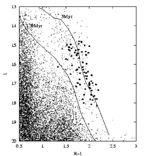
Figure 1: I,R-I colour-magnitude diagram. Spectroscopic targets are shown as follows: circles represent objects which display lithium in their optical spectra, crosses are definite cluster non-members, and our “grey area” objects are indicated by open triangles (see section 6.1). Two isochrones are shown, aged $5$ and $120$Myr, derived using the models of Baraffe et al. (1998) and assuming a distance of 352 pc and $E(R-I)=0.03$.

Our astrometry was initially performed using a nine parameter model, which included the tangent point and pincushion distortion co-efficient as free parameters. Although we finally used the SuperCosmos sky survey (Hambly et al. 2001) as our reference catalogue, the stars were so sparse in the parts of pointing 8 (see Table 1) in the direction of the molecular cloud, that for this pointing only, our initial solutions were with respect to the 2MASS survey (Cutri et al. 2003). We found the mean of the distortion co-efficients derived from each CCD image was close to the nominal value, so we fixed its value at the nominal 220. We then fitted again to find the tangent points for each CCD image, which we then averaged to find a tangent point for each pointing. With these parameters fixed, final astrometric solutions with respect to SuperCosmos (with just six free parameters) were found. The RMS deviation from the astrometric solutions for each CCD ranged between 0.13 and 0.20 arcsec.

To correct our optimal fluxes to those that would have been obtained from a large aperture we used second and third order polynomials to model the profile-correction in the directions of the short and long axes of the CCDs respectively (see Naylor et al. 2002). The photometric co-efficients used to convert the profile corrected magnitudes to apparent magnitudes were derived from observations of over 700 standard stars in $R$ and $i$ during the 4 photometric nights of the run (Landolt 1992). These were used to obtain extinction co-efficients (1 per night), colour co-efficients (1 per CCD) and zero points (1 per CCD per night). However, the small range of airmasses we observed at (1.1 to 1.5) meant that we fixed the extinction at the La Palma mean values (0.04 in $I$, 0.05 in $R-I$). We found we had to add a large systematic error (0.04 mag in $I$ 0.06 mag in $R-I$) to obtain a reduced $\chi^{2}$ of 1 for the fit. After doing this, our final number of standard stars used was 653 (8 clipped out) in $R-I$ and 720 (5 clipped out) in $I$. Note that although we used a Sloan $i$ filter, the magnitudes we derived are tied to the Landolt standards and so they are on the Cousins system.

The resulting apparent magnitudes could then be compared for stars which fell in more than one CCD field. From the stars in each overlap region we calculated a mean difference for that overlap. We then adjusted the zero points to minimise the differences, obtaining a root-mean-square (RMS) discrepancy of 0.007 and 0.008 mags in $I$ and $R-I$ respectively. Where a CCD had no overlaps, its photometry was adjusted by the mean correction for that pointing, to maintain consistency. Finally, the mean magnitude was calculated for stars appearing in two or more CCD fields.

As explained in Naylor et al. (2002), the overlaps are a powerful diagnostic of the accuracy of the photometry, since they test errors in profile correction and large-scale flatfielding, in addition to any change in transparency. They represent a very good measure of the likely photometric error. In this case, before we adjusted the zero points, we found a RMS difference of 0.05 mags between the overlaps. Since this closely matches the systematic error we had to add to the standard stars, we believe this represents our photometric accuracy. We regard this as rather poor, and are unsure of why this is so. Some of the error is due to differences between our filters and those used to create the standard star system. Specifically, we have used a Sloan $i$ filter, whilst the Landolt standards are for $I$. However, this is unlikely to be the entire cause of the problem, since a linear fit of $R-I$ vs $R-i$ for the stars of Smith et al. (2002) gives an RMS of 0.026 mags. In other work, using the same software, we have found much smaller differences between the magnitudes of stars measured in different CCD pointings (Naylor et al. 2002; Burningham et al. 2003). This suggests to us that the remaining problem originates in the flatfield, although we cannot prove that it is not the profile correction which is at fault. Our defringing technique did not entirely remove the fringes, leaving structure on a similar scale to our sky background boxes. This means the sky subtraction is not perfect, which increases the uncertainties in our photometry beyond those given by the optimal extraction. Experiments with photometry of empty regions of sky showed that the uncertainties we quote should be increased by a factor of about 1.5.

We compared our catalogue with that of Béjar et al. (2001). After applying a shift of 1.3 arcsec in RA and 1.1 arcsec in declination to our catalogue, we found good correlations out to 5 arcsec, with an RMS separation of 1.8 arcsec between the two catalogues. Our small astrometric RMS with respect to SuperCosmos suggests these numbers represent systematic shifts and uncertainties in Béjar et al.’s astrometry. Choosing just the objects with a signal-to-noise ratio greater than 10 in both catalogues, we found $I-I_{Bejar}=-0.12\pm 0.04$ and $(R-I)-(R-I)_{Bejar}=-0.07\pm 0.04$. There were no significant colour terms, but the range of colours used is small (just the PMS). Of more concern is the scatter in the relationships, with the RMS difference between measurement’s of the same star in the two catalogues being 0.24 magnitudes in $I$ and 0.13 magnitudes in $R-I$. Of course some of this scatter is likely due to variability as most of the comparison stars are probably PMS objects that are young, rapidly rotating and magnetically active, possibly with accretion discs (see Scholz & Eislöffel 2004).

3 Spectroscopy

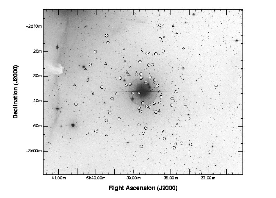
Figure 2: Digital Sky Survey image of $\sigma$ Orionis. The positions of spectroscopic targets are marked. The symbols have the meanings described in the caption to Figure 1.

3.1 Target selection

Our spectroscopic targets have been selected on the basis of their position on the $I,R-I$ colour-magnitude diagram (CMD), see Figure 1. We chose objects that were reasonably close to a 5 Myr isochrone, generated from Baraffe et al. (1998) models, using an empirical colour-effective temperature relationship derived from Pleiades data and an assumed distance of 352 pc (see Jeffries, Thurston & Hambly 2001 for details of the technique). The corresponding objects are highlighted on a Digitized Sky Survey (DSS) image in Figure 2. Targets with $14.8<I<18.2$ (corresponding approximately to masses $0.04<M<0.3\,M_{\odot}$ using a fixed age of 5 Myr, a distance of 352 pc and the Baraffe et al. 1998 models) were chosen from the catalogue with the aim of maximising the number of targets close to the cluster isochrone that could be observed in a pair of multi-fibre setups (see below). Note that because of the limited number of spectrograph fibres and other geometric restrictions (see below) we were unable to place fibres on all the good cluster candidates in the field of view (see also section 6.3).

Unfortunately IR photometry was unavailable at the time at which the spectroscopy was performed, but was later obtained for all our targets from the 2MASS all-sky point source catalogue (Cutri et al. 2003).

3.2 Spectroscopic Observations

Spectra were obtained with the Wide Field Fiber Optic Spectrograph (WYFFOS) mounted at the Nasmyth focus of the 4.2-m William Herschel Telescope during the nights of 11 and 12 December 1999. An echelle grating and order sorting filters were used to obtain spectra for targets in a field of diameter just less than 1 degree (see Fig. 2), covering wavelength ranges of $6390-6810$Å and $7820-8460$Å and at dispersions of 0.43Å pixel^-1 and 0.63Å pixel^-1 respectively. Measurements of arc-line spectra showed that FWHM resolutions of $\sim 0.9$ and $1.3$ Å  were attained with these two settings. WYFFOS had about 100 active fibres which could be allocated, but restrictions on the fibre placement and fibre proximity meant that not all of these could be used. Different fibre/target configurations were used on the two nights, with 19 (predominantly faint) objects common to both configurations. The optical fibres had a diameter of 2.7 arcsec and to estimate the co-temporal sky spectrum we allocated 15 fibres in each configuration to blank sky regions.

A log of the spectroscopic observations is given in Table 2. In addition to several hours of target exposures on each night we obtained observations of a tungsten lamp to aid in fibre location and flat fielding, Copper plus Neon arc lamp spectra for wavelength calibration at the end of each target exposure, several offset exposures of blank sky that were median stacked to calibrate the fibre-to-fibre transmission efficiencies in each configuration and wavelength setting, spectra of a number of M dwarfs that can be used as spectral-type and radial velocity standards and a spectrum of a bright, B3V star (HR 5191) that was used to identify and correct for telluric absorption lines.

(a) Sample of optical spectra displaying the Li i line at $6708$Å. Spectra are normalised within the region $6700-6715$Å prior to a constant offset being applied, labels are as given in Table 6. The gaps in the spectra correspond to a poorly subtracted bright S ii sky line at 6717Å.

(b) Near-infrared spectra showing the 8183,8195Å  Na i doublet. The dashed spectra are of the M6V field dwarf GL412b to demonstrate the difference in equivalent widths. Spectra are normalised using the region 8160-8220Å and a constant offset applied, labels are as given in Table 6.

Figure 3: Sample optical and near-infrared spectra.

Table 2: WYFFOS observing Log. Different fibre configurations were employed on the two nights, indicated by the subscripts.

	Target	RA	DEC	Central wavelength	Exposure
		(J2000)	(J2000)	(Å)	(s)
1999-12-11	$\sigma$-Ori1	05 38 43.44	-02 36 05.0	6646	3600
	$\sigma$-Ori1	”	”	6646	3600
	$\sigma$-Ori1	”	”	6646	3600
	$\sigma$-Ori1	”	”	6646	4500
	$\sigma$-Ori1	”	”	8202	1800
	$\sigma$-Ori1	”	”	8202	1800
1999-12-12	$\sigma$-Ori2	”	”	6649	4500
	$\sigma$-Ori2	”	”	6649	4500
	$\sigma$-Ori2	”	”	6649	3600
	$\sigma$-Ori2	”	”	6649	3000
	$\sigma$-Ori2	”	”	8200	2400
	$\sigma$-Ori2	”	”	8205	1800
	$\sigma$-Ori2	”	”	8205	1800
	GL 273	07 24 37.89	05 20 12.2	8199	20
	GL 388	10 19 28.69	19 52 36.9	8199	20
	GL 406	10 56 21.54	07 01 16.4	8199	240
	GL 285	07 44 33.06	03 33 40.5	8199	40
	GL 412b	11 05 21.28	43 31 35.2	8199	120
	GL 447	11 47 37.03	00 48 37.6	8199	40
	GL 1156	12 18 52.02	11 07 53.4	8199	120
	HR 5191	13 47 20.37	49 19 14.6	8199	4

3.3 Data Reduction

Images were processed using several packages from within the iraf environment. Most notable of these was wyf_red (Lewis 1996), a script based on the fibre reduction package dofibers, but with some differences. In particular, wyf_red performs CCD processing itself if provided with bias frames and flat fields. Complete reduction involved several additional tasks, the most important of which are detailed below.

1. Cosmic rays were removed automatically from target frames but a manual inspection of the arc lamp exposures was required to avoid the algorithm mistaking arc lines for cosmic rays.

2. Scattered light was subtracted by fitting a smooth function to the light found between the fibres and then interpolating this to the regions occupied by the fibre spectra.

3. The spectra were extracted using an optimal algorithm which gave more weight to regions of the profile with relatively high signal-to-noise ratio (SNR).

4. Each fibre has a different transmission efficiency. wyf_red uses the offset blank sky spectra to normalise the fibre responses and also correct for vignetting.

5. Copper-neon arc lamp spectra were used to determine a (fourth order) polynomial dispersion function for each fibre. The RMS residuals to the arc line fits were typically found to be 0.005Å  and $0.02$Å  in the optical and near-infrared regimes respectively.

6. All the derived spectra for a target obtained on one night were co-added. If an object was observed on both nights then these spectra were also co-added to find the equivalent widths (EWs) of diagnostic lines, but the separate spectra from both nights were retained to obtain two independent radial velocities (see section 4.1).

A sample of the reduced optical and near-infrared spectra are given in Figs. 3(a) and  3(b) respectively. SNR per pixel was empirically estimated by measuring the residuals to first order polynomial fits to pseudo-continuum windows. These values are conservative, as we know that many small molecular lines are probably present in these regions. In the $6690-6714$Å  region the SNR (per pixel) ranges from 3 to 20, with a median of 8. Similarly spectra in the $8175-8210$Å  window had a SNR range of 4 to 21 with a median of 9.

One anomaly which requires comment is that during the reduction we found that two of the fibres allocated to blank sky were seen to yield spectra with strong lithium absorption features! We surmised that there was an error in the translation table which relates allocated fibre numbers to spectrograph apertures. This hypothesis was confirmed by examining archival WYFFOS data and shown to apply to five pairs of fibres. We have subsequently been able to remove this source of error from our observations, and mention it here for the benefit of those who intend to make use of AF2/WYFFOS data (large fibres bundle) in the future.

4 Results

4.1 Radial Velocities

Figure 4: Errors introduced into radial velocity measurements by cross-correlating against a specific template spectrum. Residuals are the difference between the velocity derived using a specific template and the mean velocity from all five templates. The dashed line represents a residual of zero in each panel.

Figure 5: Heliocentric radial velocity (RV) as a function of $I-J$ colour. $\sigma$ Orionis non-members are marked through with crosses, “grey area” objects are triangles (see section 6.1). The 19 objects which were observed during both runs have the two velocities indicated (shown as dashed error bars); those for which only one velocity is available are shown as solid lines. The error bars are $1\sigma$ values, the cluster mean is indicated by a horizontal line at velocity $31.2$kms^-1.

Radial velocities were calculated by cross-correlating the region 8150-8250Å , which included the prominent Na i  absorption doublet (although it is weaker than the standard stars in almost all our target spectra – see section 4.2), against five radial velocity standards (see Table 3 for details). This spectral window does contain telluric absorption which could potentially alter derived radial velocities and Na i  EWs. We removed this contamination to first order by creating a calibration spectrum from the assumed smooth continuum of the B3V star we observed. The calibration spectrum was scaled according to the average airmass of observation (using the figaro program bsmult) and used to multiply the target spectrum. After this correction, very little telluric contamination could be seen.

Table 3: M-dwarf spectral type standards. $R-I$ and $I-J$ colours are taken from Leggett (1992), heliocentric velocities from Nidever et al. (2002).

Object	Sp.	R-I	I-J	RVH
(GL)	Type			(kms-1)
273	M3.5	1.55	1.49	18.2 $\pm$ 0.1
285	M4.5	1.69	1.61	26.5 $\pm$ 0.3
388	M3.5	1.42	1.35	12.4 $\pm$ 0.1
406	M6	2.18	2.33	19.5 $\pm$ 0.1
412b	M6	2.10	1.97	–
447	M4	1.68	1.65	-31.1 $\pm$ 0.1

The spectra were cross-correlated using the iraf package fxcor (Kurtz & Mink 1998). The spectra were rebinned to a log-linear dispersion and then continuum subtracted. The ends of each spectrum are forced to zero with a cosine bell function prior to a fast Fourier transform being performed. A filter is applied to the Fourier transforms to limit the frequency window used in the cross-correlation. The measured cross-correlation lags gave radial velocities which were then heliocentrically corrected according to the time of observation and the radial velocity of the standard (see Table 3).

To check the success of the cross-correlation process, we investigated the effect that using a specific standard star had on:

1. the cluster mean,

2. the scatter of objects about this mean.

This was done by cross-correlating all objects against each template spectrum after which, a mean velocity per object was calculated. The deviation from this mean when each of the templates was used is plotted as a function of $I-J$ (a good proxy for spectral type) in Fig. 4.

The top panel suggests that at the time of observation, GL447 had a velocity discrepant by about 2 km s^-1 from that given in Nidever et al. (2002). It is also clear that there is more scatter in the RVs determined from GL 285. In what follows we use the average RV obtained from cross-correlation versus the spectra of GL273, GL388 and GL406 as there seems to be little or no dependence of derived radial velocity on spectral type.

Radial velocity errors were estimated by fxcor. We tested their validity by generating three-hundred template spectra which were perturbed and degraded to simulate SNRs per pixel of 7, 15 and 25. These simulated spectra were cross-correlated with the original spectrum from which they were created. This allowed us to make an estimate of the error introduced by varying SNRs. From these simulations we concluded that the fxcor uncertainty estimates were too small by a factor of $\sim 1.75$, which was approximately independent of SNR. To remedy this, all the cross-correlation RV errors were increased accordingly. An estimate of any remaining error, as a result of spectral type mis-matches between the object and template spectra was determined from Fig. 4. The mean standard deviation in the RVs derived from each standard of 0.9kms^-1 was added in quadrature to all RV uncertainties prior to cluster membership determination. External errors, which must be considered if comparing our results with other published data, can be estimated from the deviations of the standard star RVs from their published values when their RVs are determined by cross-correlation against the other three standards (GL 447 is clearly discrepant and excluded). We estimate that any external error is less than 1 km s^-1.

Radial velocities for all objects are listed in Table 6 and displayed in Figure 5 as a function of $I-J$ colour. Those objects with two independent RV measurements from different nights are shown with dashed lines. We have observed one object (target $60=$ SOri 27) in common with Zapatero Osorio et al. (2002), three (targets $39,55,75=$ SOri 12, 29, 40) in common with Muzerolle et al. (2003), and one (target 44) which appears in Burningham et al. (2004). Table 4 compares the velocities determined by these authors with the current work. Our results concur with the literature in the cases of targets 44, 55 and 60 whereas both targets 39 and 75 display evidence for binarity in the form of a variable radial velocity. However, for consistency, they are classed as single from the data in this paper (see section 5.1).

Table 4: Radial velocity comparisons between this work [K04] and values in Zapatero Osorio et al. (2002) [Z02], Muzerolle et al. (2003) [M03] and Burningham et al. (2004) [B04]. Objects are identified as in Table 6.

	Radial Velocity (kms-1)
ID	Z02	M03	B04	K04
39		29.8 $\pm$ 0.7		37 $\pm$ 2
44			31.1 $\pm$ 4.1	34 $\pm$ 3
55		27.1 $\pm$ 1.6		28 $\pm$ 4
60	35.5 $\pm$ 10			47 $\pm$ 5
75		32.5 $\pm$ 3.3		55 $\pm$ 9

4.2 Lithium & Sodium

Figure 6: Lithium I (6708Å) equivalent width versus $I-J$ colour for our objects. Where no lithium line was observed, 2$\sigma$ upper limits are shown.

Figure 7: Sodium I (8183,8195Å) equivalent widths versus $I-J$ colour. Filled diamonds indicate our standard star measurements, open diamonds represent M-dwarfs from Xu (1991) and triangles are M-dwarf measurements from Martín et al. (2004). Objects lying below and to the right of the dashed line are considered to have gravities lower than field M-dwarfs.

The EWs of both the Li i  6708Å line and Na i  near IR doublet at 8183, 8195Å can be used as indicators of age and hence membership in samples of VLMS and BDs (see section 5). A low-order polynomial function was used to normalise the spectra using pseudo-continuum regions around both of these features (and estimate the SNR). The absorption lines were modelled as simple Gaussian functions (two Gaussians in the case of the Na i  doublet) and the results integrated to estimate the EWs. 1-sigma uncertainties in the EW measurements were estimated as

$$\delta EW=\frac{\sqrt{{\rm FWHM}\times p}}{SNR}\,,$$ (1)

where FWHM and $p$ are the full width half maxima and pixel size respectively, in units of Å. The pseudo-continuum regions either side of the lines are large enough that the statistical errors due to the uncertainty in the continuum level are negligible. The Na i  EWs for the field M-dwarf (RV) standards were also measured in the same way.

Figures 6 and 7 show the lithium and sodium EWs plotted as a function of $I-J$ colour. Where no significant Li i  feature was seen, 2-sigma upper limits to the equivalent width have been calculated based on a the median line FWHM and the SNR of the spectrum in question. This allows the distinction to be made between poor SNR spectra which may be masking the lithium line and objects which certainly do not possess the line. It is worth emphasizing that although bright forbidden lines of S ii produce a very noisy sky subtraction at 6716/6731Å, the sky background at $\pm 5$Å from the Li i  6708Å line is low and well behaved (see Fig. 3).

Our survey includes a handful of objects which have had their Li i  and Na i  features measured by other authors (Béjar et al. 1999; Zapatero-Osorio et al. 2002; Muzerolle et al. 2003). A comparison of the EWs is presented in Table 5. There is reasonable agreement between our Li i  EWs and those found in the high resolution spectra of Muzerolle et al. (2003). However, there are some clear discrepancies between our EW values and those found in lower resolution spectra by Béjar et al. (1999) and Zapatero-Osorio et al. (2002).

Table 5: Sodium I and Lithium I equivalent widths for objects common to Béjar et al. (1999) [B99], Zapatero Osorio et al. (2002) [Z02], Muzerolle et al. (2003) [M03], Burningham et al. (2004) [B04] and the current work [K04]. Objects are identified as in Table 6. Uncertainties for the equivalent widths are $\pm 1$Å  for the [B99] sample, $\pm 0.09$Å  for the [Z02] point and $\pm 0.39$Å  for the [B04] object.

	EW(Na i  )			EW(Li i  )
ID	B99	B04	K04	Z02	M03	K04
39	2.5		2.23$\pm$0.20		0.6	0.54$\pm$0.06
44		2.65	2.54$\pm$0.18
55	2.2		1.82$\pm$0.20		0.6	0.32$\pm$0.14
60	$\leq 1.0$		2.86$\pm$0.20	0.74		0.31$\pm$0.06
68	$\leq 1.0$		3.68$\pm$0.31
75	$\leq 1.0$		1.15$\pm$0.60		0.5	0.66$\pm$0.20

4.3 H$\alpha$

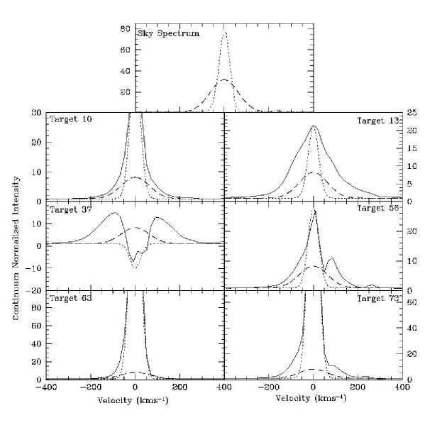
Figure 8: H$\alpha$ velocity profiles of candidate accreting objects. The top panel shows a typical sky profile (dotted line), plus a Gaussian profile (dashed line) with equivalent width $25$Å and a full width at 10 per cent of peak of $\pm 135$ km s^-1. Each subsequent panel also shows the observed H$\alpha$ line (with continuum normalised to unity), with an overplotted sky spectrum (scaled to the peak H$\alpha$ flux) and a minimal accretion profile (the dashed Gaussian) to illustrate that the profile is (a) broader than any possible contribution from the sky and (b) broader or stronger than the minimum expected profile from any accreting object.

Strong H$\alpha$ emission is a characteristic of young stars, both as a result of magnetic chromospheric activity and from continuing accretion. Our attempts to study H$\alpha$ in the $\sigma$ Ori candidates are hampered by the presence of strong, spatially varying H$\alpha$ emission that can be clearly seen in our $R$-band images and is presumably associated with hot gas in the line of sight towards $\sigma$ Ori. The signal from the background H$\alpha$ is very strong and, in our 2.7 arcsec diameter fibres, swamps any H$\alpha$ signal from the targets, making a measurement of the H$\alpha$ EW impossible. However, the background emission is unresolved in our sky spectra, with a FWHM of about 40-50 km s^-1. White and Basri (2003) have demonstrated that H$\alpha$ emission lines formed by accretion processes should be much broader than this. Classical T-Tauri stars typically exhibit H$\alpha$ lines with a full-width at 10% of the peak emission of $>270$kms^-1. So, whilst we cannot measure the strength of the H$\alpha$ line, we can certainly search for emission wings extending to more than $\pm 135$ km s^-1 from the line centre, which are uncontaminated by the background H$\alpha$ emission.

The H$\alpha$ EW expected from accreting objects which demonstrate extended H$\alpha$ emission with spectral types M3-M7 (the approximate range of our sample) is greater than 25Å and more usually several times stronger (e.g. see White & Basri 2003; Muzerolle et al. 2003). Given the dispersion of our spectra and assuming the H$\alpha$ profile is pseudo-Gaussian it is easy to show that such a line would produce a signal of strength $>0.7$ times the continuum level at $\pm 135$ km s^-1 from the line centre. Such a signal should be easily detectable if present, even in our poorest spectra.

Analysis of our spectra yields five objects which clearly exhibit extended H$\alpha$ emission on this basis (see Fig. 8) and a further one (target 63) which has a marginally broadened line which may simply be a case of poor sky subtraction or the result of small changes in the instrumental dispersion profile over the detector. These objects are marked with an “a” in the last column of Table 6.

5 Membership

Determining the membership status of candidates can be a subjective process largely dependent on the specific criteria set. This section details the three diagnostic tools we used to assign membership of the $\sigma$ Orionis cluster.

5.1 Radial Velocities

Our initial indicator of cluster membership was based on comparing individual RVs to the weighted mean cluster velocity. Targets lying more than $3\sigma$ away from this mean were flagged as likely non-members (or binaries) and excluded from subsequent recalculations. In the $19$ cases where two RVs were available for a given object, the average of the two was used in computing the ensemble velocity. The result of this iterative process was that $66$ objects were designated as $\sigma$ Orionis RV cluster members, lying within $3\sigma$ of a cluster mean velocity of $31.2\pm 0.2$ km s^-1 (which has an additional external error of up to 1 km s^-1).

Our mean RV for the cluster agrees reasonably well with the systemic velocity found for $\sigma$ Ori by Morrell & Levato (1991) of 27 km s^-1; the value of $29.1$ km s^-1 listed for $\sigma$ Ori by Evans (1967); the peak in the RV distribution of low-mass PMS candidates around $\sigma$ Ori at 25-30 km s^-1 found by Walter et al. (1998) and at 29.5 km s^-1 by Burningham et al. (2004). It is somewhat lower than the mean of 37.3 km s^-1 reported for a group of candidate low-mass members by Zapatero-Osorio et al. (2002).

The iterative clipping process has the potential to exclude candidate members which are cluster binary systems with a small enough separation to introduce RV variations that move them away from the cluster mean. If other information suggests strongly enough that candidates are indeed $\sigma$ Ori association members, then a single discrepant RV measurement can be sufficient to identify a short period, single-lined spectroscopic binary. So, all objects failing the RV test must be examined closely for any convincing signs of membership from other indicators.

From these considerations we have 10 RV non-members in our sample, with heliocentric RVs ranging from -25 to 120 km s^-1. If we approximate our RV selection to a band of width $\sim 25$ km s^-1 centred on the cluster mean and assume that contaminating RV non-members are spread evenly in RV space then we would only expect of order 1-2 contaminating non-members to be left among our RV-selected members.

5.2 Sodium

Each of our $\sigma$ Ori candidates exhibits the gravity sensitive $8183,8195$Å  sodium doublet in their near-infrared spectra. The strength of this doublet is gravity sensitive (see Schiavon et al. 1997). It is 2-3 times stronger in cool M dwarfs (M4 and later) than in PMS stars with age $<10$ Myr and similar effective temperature (e.g. Kirkpatrick et al. 1991; Martín, Rebolo & Zapatero-Osorio 1996; Martín, Delfosse & Guieu 2004). As demonstrated in Figure 7, this test may only be conclusive for objects with $I-J>1.6$. Warmer objects in the $\sigma$ Ori cluster will have gravities only slightly lower than field objects with the same colour. We define an arbitrary empirical boundary, plotted on Figure 7 with a dashed line, below which we are confident that a low Na i  EW indicates a gravity consistent with PMS status. 64 candidates lie below this line and $12$ above.

The Na i  EW is also very weak in giant stars ($\leq 1$Å according to Schiavon et al. 1997), but contamination of our sample by M-type giants is highly improbable. An M-giant at the appropriate location on the CMD would have an absolute $I$ magnitude $<-2$ and hence would have to be at distances $>25$ kpc. As the galactic latitude and longitude of $\sigma$ Ori are $l=206.8^{\circ}$, $b=-17.3$, such objects would be more than 7.4 kpc below the galactic disc, where their spatial density is known to be essentially zero (Branham 2003).

5.3 Lithium

The presence of undepleted lithium should be an excellent indicator of stellar youth, because it is burned in the fully convective interiors of low-mass PMS stars once their cores reach a threshold temperature. We would expect Li to start being depleted by more than a factor of 100 among contaminating field VLMS at ages between 20 Myr (at 0.35 $M_{\odot}$) and 120 Myr. Field BDs with masses below about 0.06 $M_{\odot}$ never deplete Li, but these would have colours redder than $I-J>2.8$ (the reddest in our sample) for ages $>140$ Myr (Baraffe et al. 1998). According to tables of EW versus Li abundance presented by Zapatero-Osorio et al. (2002), which have appropriate temperatures for the sample considered here (at 5 Myr $1.4<I-J<2.8$ corresponds to $3500>T_{\rm eff}>2650$ K – Baraffe et al. 1998), undepleted Li should result in a Li i  6708Å line EW of about 0.5-0.6Å  falling to 0.2-0.3Å after a factor of 100 depletion and becoming much weaker shortly after that. Thus the detection of Li i  6708Å consistent with an EW of 0.2Å or more should be a very strong indicator of youth in the hottest stars of our sample (implying ages $<20$ Myr), but is less constraining (ages $<140$ Myr) for the coolest stars in our sample. Only a small fraction ($\simeq 0.1-1$ per cent) of any contaminating foreground field stars might be expected to show evidence for Li at this level.

A caveat to this picture might be if there are remnants from an older generation of star formation in the Orion region which might show Li. However, these older stars would have to lie in the foreground (to appear in the CMDs in the correct place) and would also have to satisfy the RV tests to be included as candidate members. We have to bear in mind that potential binary members exhibiting Li, and a weak Na i  feature but with a discrepant RV could also be members of a young (10-100 Myr) foreground population.

Figure 6 shows the $57$ objects with available equivalent widths (and photometry) along with $19$ calculated upper limits. We decide to rule out membership for any star which has EW[Li]$<0.2$Å  at the 2-sigma level. Above this level the presence of Li is taken to be very strong evidence of cluster membership and if the Li measurement upper limit is inconclusive then the evidence from the other two membership indicators is used. However, we find a number of objects that display weak or absent Li but which appear to have low-gravity and are RV members and we will return to these in Section 6.

6 Discussion

6.1 Membership Indicators

Using three membership tests means that candidates can be placed into a number of categories.

1. Most candidates ($55/76$) are RV members with weak gravity and display evidence of significant lithium in their atmospheres. These are clearly the strongest cases for being true $\sigma$ Ori members. All but one of the strong H$\alpha$ emitters/accretors belong in this category.

2. There are 3 candidates (targets 27, 40 and 73 – an H$\alpha$ emitter/accretor) which have an inconclusive upper limit to their Li EW, but which are RV members and display low gravity.

3. There are 3 candidates that display a low gravity, are RV non-members and either show Li (targets 46 and 74) or have an upper limit to their Li consistent with the presence of significant Li (target 72). These are possible binary members of the cluster. In the case of target 72, the RV is demonstrably variable.

4. There are 8 candidates which have no Li, are RV members and have a Na EW that is either inconclusive (targets 29, 33, 34, 45, 53 and 59) or indicates a low gravity (targets 25 and 76).

5. There is 1 candidate (target 52) which shows no evidence for Li, has a discrepant RV yet a weak Na EW, indicative of low gravity.

6. There are 6 candidates (targets 7, 12, 26, 28, 30 and 38) that have very low upper limits to their Li EW, inconclusive Na EW and highly discrepant RVs. These are all considered definite non-members

In summary we have found what we believe are 57 firm members of the $\sigma$ Ori cluster (those displaying Li), of which 2 are probable short period binary systems. We have also identified 6 objects as clear non-members of the cluster. Inevitably some of our classifications are arguable, but there is sufficient information in Table 6 for the reader to generate their own classifications.

Thirteen of our targets (an uncomfortably large number) lie in a grey area where we find it difficult to assign membership, either because they show low-gravity but discrepant RVs, low-gravity but no Li, or the right RV but no Li. Only 2 out of these 13 show discrepant RVs, one of which is definitely an RV variable. Given the relatively narrow range of RVs occupied by members and the spread of velocities occupied by the 10 (out of the total 76) targets with discrepant RVs, we would only have expected 1-2 non-members to have the “correct” RV. This presents us with a puzzle, because it suggests that the majority of the 11 “grey area” objects with the “correct” RV should be cluster members. Three of these objects have an upper limit to the Li EW which could be consistent with negligibly depleted Li, but 8 do not, and of these, 2 (targets 25 and 76 – see Fig. 3(a)) have a small Na EW that would seem to unambiguously classify them as low gravity PMS objects. This in turn suggests there may be a problem in using a simple EW[Li] threshold to discriminate between cluster objects and non-members. On the other hand, that 2 out of 13 grey area objects are RV non-members contrasts with only 2 out of 57 Li-rich RV non-members. So unless short period binarity somehow has a tendency to reduce EW[Li], it is probable that one or more of these 2 are not cluster members, despite appearing to be low-gravity objects (see also section 6.4); in which case we have the problem that EW[Na] may not be a foolproof membership indicator.

6.2 A spread in Li equivalent widths?

Figure 9: $I$,$I-J$ colour-magnitude diagram. Symbols have the same meaning as in Fig. 1 with open squares around those objects found to have accretion. Evolutionary tracks for masses $0.04-0.6$M_☉ (dotted lines) and isochrones for ages $1-50$Myr (dashed lines) are calculated using the models of Baraffe et al. (1998). The isochrones range from 1 Myr (far right) to 50 Myr and the evolutionary tracks are shown for masses from 0.6 $M_{\odot}$ (at the top) to $0.04\,M_{\odot}$.

We have observed a large spread in the measured values of EW[Li]. The spread appears to be confined to those cluster candidates with $I-J>1.7$ (see Fig. 6) and cannot be explained with the quoted experimental errors – many of our spectra are of reasonably high quality and we believe the statistical errors in the EW values are quite robust, if not pessimistic. In particular there appear to be a substantial fraction of the cooler stars which have EW[Li]$\sim 0.3$Å. In addition there are also the “grey area” objects, the majority of which are likely to be members but most of which appear to exhibit no Li (including three with a definite PMS gravity).

It also seems that the average EW[Li] declines with increasing $I-J$ from about 0.6Å to 0.5Å across our full $I-J$ range. We mention this because the tables of EW versus Li abundance presented by Zapatero-Osorio et al. (2002) show instead a slight increase in the expected EW[Li] for an undepleted Li abundance, of about the same magnitude. A plausible explanation for the decreasing average EW[Li] with $I-J$ in our sample arises from the definition of the pseudo-continuum used to estimate EW[Li]. The continuum regions we have used cover a rather wide range around the Li feature, so they must surely contain molecular absorption features which become stronger at cooler temperatures. This would depress the pseudo-continuum leading to lower estimates of EW[Li].

A real Li abundance spread could be caused by depletion as Li is burned in the cores of contracting young low mass objects. As explained in section 5.3, factors of 100 depletion in Li are probably needed to reduce EW[Li] to $\leq 0.3$Å, which does not occur (according to the models of Baraffe et al. 1998) until ages of 20-120 Myr. Other models, such as those of D’Antona & Mazzitelli (1997) or Siess, Dufour & Forestini (2000), predict similar if not slightly larger timescales for Li depletion. Figure 9 shows the $I$ versus $I-J$ colour magnitude diagram for our targets together with isochrones from the Baraffe et al. (1998) models. The models are adjusted for the Hipparcos distance to $\sigma$ Ori of 352 pc and suggest a spread of ages between $<1$ and 20 Myr for our Li-confirmed cluster candidates. Only some of the oldest, most massive stars in our sample could have suffered significant Li depletion if these ages are taken literally. However, the “oldest” Li-poor cluster candidates among the bright stars in our sample also have discrepant RVs and so are almost certainly cluster non-members. In any case the apparent age spread present in the diagram is likely to be a vast overestimate – photometric variability, binarity and for some stars, the presence of discs, can perhaps entirely explain such spreads (e.g. Hartmann 2001). We conclude that Li-depletion among members of the $\sigma$ Ori cluster is unlikely to be the cause of spreads in EW[Li] unless current PMS evolutionary models have very serious flaws.

An alternate possibility is that some of our cluster candidates are genuinely depleted of Li because they are older and are not cluster members. They could belong to a foreground population of older stars that are at an appropriate distance to place them close to the $\sigma$ Ori cluster locus in CMDs (see Alcalá et al. 2000; Walter et al. 2000). Such objects would need to have a similar RV to the cluster (which is quite different to the general field population), be old enough to have depleted a factor of 100 or more of their initial Li and be yet be young enough to exhibit weak Na lines. There may be a vanishingly small range of ages that can satisfy these requirements and whilst a slightly older population (the Orion OB1a subgroup; age$~{}11$ Myr) does exist in some parts of the Orion star forming region, it is at a similar distance and there is no evidence of this older component in the direction of $\sigma$ Ori (Sherry 2003). To conclude, we find this possibility unlikely.

A second class of explanations are those in which the spread is apparent in the EWs because of deficiencies in the atmospheric analysis or the data reduction. The EW-abundance relationships we are using to interpret our results show that the EW[Li] versus $T_{\rm eff}$ relationship is quite flat over the $T_{\rm eff}$ range considered here. It is therefore unlikely that uncertainties in the colours play any significant role in the EW[Li] scatter. Likewise, temperature inhomogeneities on the stellar surfaces caused by magnetic fields are are also unlikely to have much effect. Some photospheric lines can be veiled in young stars that are undergoing accretion, but the majority of stars in our sample are accreting at a rate $M<10^{-11}M_{\odot}$/year (see section 6.5) which is insufficient to cause such an effect (Muzerolle et al. 2003). Also, the 5 or 6 objects which do show evidence for ongoing accretion have EW[Li] values of 0.32Å to 1.19Å, which are not systematically low compared with the rest of the sample.

We have also considered possible data reduction problems such as an uncertain and perhaps systematically underestimated scattered light or sky contributions which would preferentially affect the fainter targets. The level of scattered light in the spectrograph is simply too small to be of concern here. The sky contribution is more significant, but we estimate that it is subtracted with a precision of better then 5 per cent based on the scatter in the fibre-to-fibre relative efficiencies determined from three successive offset sky exposures. We have confirmed that this would not significantly increase the quoted EW[Li] uncertainties for any of our targets.

Finally we note that a spread in EW[Li] among VLMS and BDs has been seen before, although not extensively discussed. Both Jörgens & Guenther (2001) and Natta et al. (2004) have reported significant EW[Li] spreads of $<0.09$ to 0.63Å and 0.2 to 0.5Å respectively, among a small group of very low mass objects in the young Chamaeleon I cluster. It is also notable that a subset of these objects were observed earlier by Neuhäuser & Comerón (1999), albeit at lower resolution, who found quite different EW[Li] for some objects.

We can reach no firm conclusion here. The EW[Li] spread demands further attention with better spectra, if only to rule out the possibility of major problems with the current evolutionary models. Our results cast doubt on any selection technique which rules out membership of young clusters solely on the basis of a small EW[Li].

6.3 Contamination and the mass function

Previous work on the $\sigma$ Ori cluster has attempted to estimate the mass function of VLMS and BDs using photometrically selected samples, finding $dn/d\log m\propto m^{-\alpha}$, with $\alpha=-0.2\pm 0.4$ for $0.01<m<0.2\,M_{\odot}$ (Béjar et al. 1999, 2001). Only a minority of this sample have been followed up spectroscopically and in most cases, this spectroscopy is limited to obtaining a spectral type and noting the presence of moderate to strong H$\alpha$ emission in low resolution (20Å FWHM) spectra. We contend that such an approach may not yield reliable results. As we discussed earlier, the main source of any contamination in the sample will be late-type foreground M dwarfs that have spectral types, colours, and in many cases H$\alpha$ emission, that are similar to members of $\sigma$ Ori. A very large H$\alpha$ EW of perhaps 20-40Å or more is associated with accretion and hence youth, but is present in only a small fraction of $\sigma$ Ori members (see section 6.5). Measurement of radial velocities, Li and weak gravity using Na and K line strengths will be much more reliable, but is only possible with higher resolution spectra.

Arguments based upon the space density of field M dwarfs, have suggested that any contamination in a photometrically selected sample may be quite low (see Béjar et al. 1999 and below). Our spectroscopy and membership classification partially reinforce this view. We have found at least 57 (and probably closer to 64) likely members from a sample of 76 selected only on the basis of their $I$ magnitudes and $R-I$ colours. Cluster members are found close to the edge of the sample distribution in both the $I$ vs $R-I$ and $I$ vs $I-J$ CMDs, suggesting that the photometric selection criteria may have been too restrictive to include all the possible members of $\sigma$ Ori. RV measurements of another faint sample of $\sigma$ Ori candidates spread over a wider region of the $I$ vs $R-I$ CMD by Burningham et al. (2004) suggest that few members lie outside the region we have considered. However, because of this uncertainty and because we have not observed a complete sample of photometric candidates over our restricted field of view, we limit ourselves in this paper to asking whether a mass function derived solely by photometric selection is likely to be significantly affected by non-member contamination?

The definite non-members we have found are at the brighter end of the sample ($14.8<I<16.3$) – where the contamination level is 15-25 per cent (depending on the status of the “grey area objects”). Based solely on their low EW[Na], it is possible that all of the fainter objects are members, but the contamination level could be as high as 20 per cent if all the “grey area” objects turn out to be non-members. Contamination at this level would have minimal impact on the value of $\alpha$, especially when compared to the effect of statistical, distance and model-dependent uncertainties.

To check our estimates of contamination we have simulated an $I$ versus $R-I$ diagram populated by field dwarfs. The details of this simulation, which uses the local field dwarf luminosity function and space density, are presented in Jeffries et al. (2004). We simulated a 0.5 square degree field towards $\sigma$ Ori, similar to that area from which our spectroscopy targets were chosen. An $I$ versus $R-I$ diagram was generated for objects up to 500 pc distant. We then selected objects with $14.8<I<18.2$ and in a strip 0.6 magnitudes wide in $R-I$ and centred on the 5 Myr isochrone shown in Fig 1. We found that 41 simulated M-dwarfs lay within this strip. In the real photometry dataset there are 115 objects in the same strip, of which 74 were observed spectroscopically and $57-70$ are found to be members depending on the status of “grey area” objects. Hence we would expect to have observed about 25 non-members in our spectroscopic sample, compared to the 4-17 we have found. We consider this reasonable agreement, although any discrepancy might be explained by a tendency for us to prefer to allocate fibres to spectroscopic targets which lay close to the 5 Myr isochrone. Most of the contaminants will lie on the blueward side of the selected strip. Indeed only 2 simulated contaminants lay on the red side of the 5 Myr isochrone and Fig. 1 shows that all the confirmed non-members and all but one of the “grey area” objects lie blueward of the 5 Myr isochrone.

It is interesting to note that had we applied a strict age$\leq 20$ Myr criterion using the $I$ vs $I-J$ diagram shown in Fig. 9, we would have excluded all of the definite non-members from our sample. The 4 “grey area” objects that would be excluded on this basis have no Li, have an ambiguous EW[Na] and in two cases an RV only marginally consistent with cluster membership. Selection on the $I$ versus $I-J$ diagram seems therefore to have the potential for being more discriminating in choosing a sample of genuine cluster candidates.

6.4 Binarity

Figure 10: The efficiency with which we are able to detect binaries as a function of separation. The solid curve is averaged over the 57 objects in sample A (see text). A similar curve for sample B is almost indistinguishable. We have assumed circular orbits, random inclination angles, a flat mass ratio distribution for $0.2<q<1$ and primary masses taken from Fig. 9.

Figure 11: On the left we show the assumed distribution of binary separations. The top plot has a peak at 15 au and a Gaussian sigma of 1.53 in logarithmic units. They have been normalised to show the approximate binary fractions seen in sample of nearby M-dwarfs (see Fischer & Marcy 1992, figure 2), with a total binary fraction of 0.42. The bottom panel shows a flat distribution with a similar normalisation. On the right we show the corresponding probability that these distributions produce the observed numbers of binary systems. The solid curves show the results for sample A (2 binaries from 57), and the dashed curves show the results for sample B (4 binaries from 64).

The data we have obtained offer us the opportunity to investigate the fraction of VLMS and BDs in the $\sigma$ Ori cluster which are in short period binary systems. A test can be formulated to see whether the RVs of cluster members are (a) constant, if measured more than once, and (b) consistent with the mean cluster RV. The fraction of short period binaries identified in this way can then be compared with models of the binary fraction as a function of separation, $a$, and mass ratio, $q$, that also take into account the RV sampling and uncertainties.

A difficulty here is deciding which candidate VLMS and BDs to include as genuine members. Clearly we cannot use measured RV as a criterion! We make two choices, one more restrictive than the other. The first sample is all those VLMS/BD candidates which show clear evidence for Li in their spectra – a total of 57 objects, which we will call sample A. The second sample, includes the first as a subset, but also includes all those objects with an EW[Na] which would seem to unambiguously classify them as low-gravity objects – a total of 64 objects, which we will label as sample B. Since these bracket a range of possibilities for the binary fraction, we perform calculations using both.

We applied a $\chi^{2}$ test to the radial velocities of the candidate cluster members in each sample in order to identify binary systems. In effect, we were testing the goodness-of-fit of the mean cluster RV to the observed RV(s), adding the uncertainty in the cluster mean in quadrature to each error bar. The $\chi^{2}$ threshold was set so that there was a probability of $<10^{-3}$ of a constant RV cluster member failing the test. Two objects from sample A (targets 46 and 74) were identified as binary and a further 2 objects (targets 52, and 72) in sample B. Then, assuming circular orbits and primary masses taken from Fig. 9, we used the mean times of observation and the RV error bars for each target to calculate the probability that a binary RV variation would have been detected at this level, both as a function of $a$ and $q$ and averaged over all inclination angles. Summing these probabilities over all targets and over particular distributions of $q$ yields a “detection efficiency” as a function of binary separation for that particular sample. We can then calculate the probability that a given binary fraction, $q$ and $a$ distribution can result in the number of binaries observed (see Maxted et al. 2001).

As an example, Fig. 10 shows how efficiently (on average) we can detect binary systems for a given separation for samples A and B. In the absence of any definitive information on the distribution of $q$ in VLMS/BDs we assume a flat mass ratio distribution for $0.2<q\leq 1$ which is reasonably consistent with what is observed for M-dwarfs (Fischer & Marcy 1992). If the $q$ distribution were peaked towards $q=1$ then binaries become more detectable and the required binary fraction to explain a set of observations becomes lower (and vice-versa). It is clear from this plot that our survey is not sensitive to systems with separations of $\log a\ga 0$ (in au). Conversely our detection efficiency for closely separated binaries is very high.

Given the sparse nature of our RV dataset we limit ourselves to an attempt to answer one simple question. Is the number of candidate binary systems we have observed consistent with the overall binary fraction ($42\pm 9$ per cent) and Gaussian $\log a$ distribution proposed by Fischer & Marcy (1992) for M-dwarfs within 20 pc? In one sense we already know that for BDs the answer to this is no. There are too few field and cluster BD-BD binary systems with $a>20$ au compared with M-dwarf binaries in the same separation range. (e.g. Martín et al. 2003; Gizis et al. 2003). However, we are probing the small separation end of this distribution which is a separate problem. We begin by using Fig. 10 to calculate the probability that a given binary fraction would have resulted in the number of observed binary detections, as a function of $\log a$. We then convolve this with an assumed separation distribution that is a Gaussian with a peak at $\log a=1.16$ and a sigma of 1.53 (in au). The normalisation of the function is effectively set by the number of binaries we have observed. A plot of probability versus binary fraction can then be produced by integrating over any given range of $\log a$, although as the detection efficiency becomes negligible for $\log a>0$ (see Fig. 10) we confine ourselves to $-3<\log a<0$.

In the case of sample A and assuming that the Gaussian $\log a$ distribution shown in Fig. 11a is appropriate, we find that the most likely binary fraction (between $-3<\log a<0$ only) is 0.19, with a lower limit of $>0.13$ at a 90 per cent confidence level (see Fig. 11b). This is inconsistent with the estimate of about 5-7 per cent binarity for this range of $\log a$ (Marcy & Benitz 1989; Fischer & Marcy 1992) in nearby M-dwarfs. For sample B where there is an even higher observed binary fraction the probability curve peaks at a binary fraction of 0.47 and with a lower limit of $>0.17$ at a 90 per cent confidence level.

These results imply that if VLMS/BDs do have a separation distribution that decreases towards smaller separations in a similar way to field dwarfs, then we have observed too many to be consistent with the small binary fraction found for field M-dwarfs at small separations. This in turn means that either the distribution of separations is quite different in the VLMS/BDs and/or the binary fraction at small separations is very high. To test the sensitivity to the assumed distribution of $\log a$, we have performed another calculation assuming a flat distribution (see Fig. 11c). In this case sample A returns a most probable binary fraction ($-3<\log a<0$) of only 0.07, with a lower limit of 0.07 at 90 per cent confidence. So, depending on the detail of the separation distribution it seems that fraction of VLMS/BDs in short period binary systems could be quite small (if the $\log a$ distribution is much flatter than found for higher mass stars) or could certainly be as high as the 0.5 suggested by Pinfield et al. (2003) for VLMS/BDs in the Pleiades. Either way the binary properties for short-period VLMS/BDs would be quite different from those of M-dwarfs, as indeed they are at larger separations.

There are several caveats to this interesting conclusion. (i) It is based on very small number statistics, which although statistically taken account of in our calculations, render the result vulnerable to contamination of the binary sample. (ii) Greater consistency with the M-dwarf distribution would be achieved if some of the candidate binary members were not binaries. This might be the case if our RV errors were underestimated, but in that case we would be less sensitive to binaries and the deduced binary fractions would remain similar. (iii) The binary fraction would be smaller if some of the binary candidates turn out not members of the cluster. This certainly applies to sample B which contains two “grey area” binary candidates for which we are not certain of cluster membership. Indeed the large implied binary fraction could be viewed as evidence that this is the case. However our main conclusion holds even if we consider just the sample in which Li was detected. (iv) If the $q$ distribution for VLMS/BDs was sharply peaked towards $q=1$ this would make it easier to detect binaries and thus our efficiency would be greater and the required binary fraction lower.

Our results seem reasonably consistent with the survey of 26 field VLMS/BDs conducted by Guenther & Wuchterl (2003). They used 2-3 RV measurements with precision 0.1-1 km s^-1 spread over 1-2 months. They find 3 binaries in this sample and hence deduce a binary fraction of at least 12 per cent for periods of $<100$ days (roughly equivalent to 0.2 au). If we perform our calculation for $-3<\log a<-0.7$ for the case of sample A and the Fischer & Marcy (1992) distribution, we obtain a most probable binary fraction of 11 per cent. Both of these numbers should be compared with the $\sim 3$ per cent binarity implied by the Fischer & Marcy analysis over a similar separation range. To make further and more decisive progress would require a multi-epoch RV survey of a large sample of VLMS/BDs in the $\sigma$ Ori cluster and elsewhere. Observations spread over several months and with a factor of a few better precision would give sensitivity to separations as large as the minimum observable with adaptive optics systems for nearby BDs and would allow some estimation of the $\log a$ distribution.

6.5 Disc Fractions

The frequency and lifetimes of discs around young, VLMS/BDs may be an important diagnostic tool in identifying the dominant (sub)stellar formation scenario. A shorter disc lifetime for lower mass objects as a result of dynamical ejection of stellar embryos from their initial gas reservoirs is qualitatively supported by numerical models (Bate et al. 2003). Haisch et al. (2001) determined disc fractions (using $K-L$ near infrared excess) for low-mass stars (0.2-1 $M_{\odot}$) in several clusters, demonstrating a rapid decrease in disc frequency with age – initial frequencies may be as high as $\sim 80$ per cent, with approximately half of the discs being lost within $\la 3$ Myr, and an overall lifetime of $\sim 6$ Myr. Thus, at an age of $3-7$ Myr some dissipation of circumstellar discs is certainly expected within the $\sigma$ Ori cluster. Using similar diagnostics, Oliveira, Jeffries & van Loon (2004) found that $\sim 50$ per cent of low-mass stars around $\sigma$ Ori possessed circumstellar material, broadly agreeing with this scenario. Liu et al. (2003) and Jayawardhana et al. (2003b) present $K-L$ measurements for BDs in a number of clusters which support a similar timescale for disc dissipation in lower mass objects.

Five or possibly six of our very low-mass $\sigma$ Ori cluster members show evidence for the presence of accretion on the basis of broad H$\alpha$ emission. Three of these objects are probably substellar according to Fig. 9. The deduced accretion frequency of $10\pm 5$ per cent is much lower than the frequency of discs found among higher mass objects by Oliveira et al. (2004). However, different disc indicators cannot be considered equivalent. Natta et al. (2004) show that a broadened H$\alpha$ profile with a full width at 10 per cent of maximum of $>270$ km s^-1 is sensitive to accretion rates $>10^{-11}$ $M_{\odot}$ yr^-1 (for VLMS/BDs), whereas a $K-L$ excess can be seen even from a passive (reprocessed light only) disc with $M>10^{-6}$ $M_{\odot}$ (Wood et al. 2002; Walker et al. 2004). For example, 23 of the brighter objects in our sample (all with $I<16.75$) have $K-L$ measurements in Oliveira et al. (2004) or Oliveira et al. (in preparation). Of these, 6 to 9 (depending on the exact criteria) show a $K-L$ excess, but only targets 10, 13 and 37 have been identified as accretors. Jayawardhana et al. (2003b) also find that 2 out of 6 BDs in $\sigma$ Ori have $K-L$ excesses, but we have found no evidence for accretion in either of these (S Ori 12 and S Ori 40).

A more sensible comparison would be with the frequency of strong, accretion-related H$\alpha$ emission in stars of higher mass in the $\sigma$ Ori cluster and VLMS/BDs in younger and older clusters. Among younger clusters, Jayawardhana et al. (2003a) find the fraction of accreting substellar objects (based on the width of the H$\alpha$ line) to be about 50 per cent for ages $\leq 2\,$Myr (in IC 348). Muzerolle et al. (2003) measured a small sample of eight $\sigma$ Ori candidates, finding no accretors. S Ori 12, 29 and 40 are in common with this study and we also find no evidence for accretion in these objects. Neither do they find any VLMS/BD accretors in the older ($\sim 8$ Myr) Sco-Cen association. Our measurements from a much larger sample clarify this trend and pin down the accretion timescale for most VLMS/BDs to be less than the age of the $\sigma$ Ori cluster.

The H$\alpha$ results for VLMS/BDs in the $\sigma$ Ori cluster are similar to those for higher mass stars. Wolk (1996) states that 12 per cent (6 out of 49) among a sample of $\sigma$ Ori candidates with spectral types K0-M0 are classical T-Tauri stars with accretion discs, using EW$[$H$\alpha]>10$Å as his criterion. Using the same H$\alpha$ criterion, Zapatero-Osorio et al. (2002) find one star from 11 shows accretion in the same spectral type range. Among younger clusters, the preponderance of accretion-induced H$\alpha$ emission is much higher. For example, 63 per cent (30/48) stars with $M>0.2\,M_{\odot}$ are accretors in the Taurus-Auriga (age 1-2 Myr) sample of White & Ghez (2001).

Hence, it seems that, similarly to the $K-L$ disc indicator, the fraction of objects with discs betrayed by their accretion signatures declines at a rate that is roughly independent of mass, but that the decline takes place more rapidly. Interpretation of this result is complicated by the mass-dependence of the sensitivity of these tests. Most low-mass classical T-Tauri stars accrete at rates that are orders of magnitude higher than the threshold below which their accretion would be undetectable. Accreting BDs on the other hand are detected at rates right down to a smaller threshold. This suggests that the transition between accreting and non-accreting status may happen quite rapidly for low-mass stars and that the fraction of accreting BDs may be an underestimate. Either way it seems that accretion may become undetectable even whilst a significant mass of disc material is still present. If accretion at a rate $\sim 10^{-11}$ $M_{\odot}$ yr^-1 is present in BDs at an age of $\sim 5$ Myr, it implies disc masses of order $5\times 10^{-5}\,M_{\odot}$. The recent models of flared discs around BDs by Walker et al. (2004), do indeed suggest that near-IR excesses should be present for these and even less massive discs.

The presence of accretion discs in a significant fraction of VLMS/BDs at an age of a few Myr and in similar numbers to those seen in higher mass stars at the same age, does not support the idea of VLMS/BDs forming by a dynamical ejection process in which their discs are truncated. Instead it argues for a common formation mechanism for low-mass stars, VLMS and BDs. However, whether such observations can definitively rule out the ejection model must await detailed predictions of the initial BD disc properties and masses from such a scenario (e.g. see the discussion in Liu et al. 2003 and Natta et al. 2004).

7 Conclusions

We have used intermediate resolution spectroscopy to refine a set of candidate VLMS and BD members of the $\sigma$ Ori cluster (age $\sim 3-7$ Myr) that were chosen on the basis of their $RI$ photometry. We have measured radial velocities, the strengths of absorption lines due to neutral lithium and sodium and searched for signs of accretion activity.

We find that the majority of the photometrically selected candidates are genuine cluster members on the basis that they exhibit an Li i 6708Å absorption feature, have radial velocities consistent with cluster membership and have a Na i 8183/8195Å absorption doublet that is weaker than main sequence M-dwarfs of a similar spectral type. The cluster members we have identified have model- and distance-dependent masses of $0.03<M<0.35\,M_{\odot}$. Approximately 23 of our targets are likely to have substellar masses when measured in this way.

We have found another class of candidate where the evidence is ambiguous. These objects either have upper limits to their Li line EWs that may be consistent with cluster membership, have radial velocities that indicate they are non-members or cluster binaries or have no Li but radial velocities consistent with cluster membership. Several of these objects have weak Na i absorption that indicates a youthful status. These objects, together with the apparent spread in the strength of the Li i 6708Å absorption EW among cluster members, lead us to conclude that there may be deficiencies in our understanding of the formation of this feature in cool, low gravity objects. It may be unsafe to rule out the membership of a VLMS or BD from a young cluster or association solely on the basis of a weak or absent Li feature.

Despite these problems we find that overall, photometric selection alone is reasonably effective in isolating members of the $\sigma$ Ori cluster. We estimate contamination rates of 15-25 per cent among the higher mass stars of our sample and $<20$ percent at the lower mass end. Contamination at this level will not significantly change the form of the cluster mass function that has been deduced from photometrically selected samples. However, we do show that selection in the $I$ versus $I-J$ diagram is potentially more discriminating than the $I$ versus $R-I$ diagram.

We have identified 4 candidate binary cluster members on the basis of a varying RV or an RV discrepant from the cluster mean combined with other indications of membership. Two of these candidates show signs of Li in their spectra. A careful consideration of the RV errors and sampling in our data enables us to determine how efficiently we can detect binary systems as a function of primary mass, mass ratio and separation. Combining this calculation with the number of binaries we have observed and plausible distributions of binary mass ratio and separation, we determine that we have found too many binary systems to be accounted for by binary properties similar to those in higher mass stars. Instead, the short-period binary frequency could be much larger in our VLMS/BDs (perhaps as high 0.5 for $-3<\log a<0$) or the binary frequency is lower but the distribution with $\log a$ must be flatter than seen in higher mass field M-dwarfs. Caveats to this conclusion must be considered. The results are crucially dependent on the correct identification of a small number of binary members of the cluster. However, these conclusions still apply even if we restrict ourselves to considering cluster members where the presence of Li has been positively identified. Further work will be needed to hone this result – a multi-epoch RV survey of a large sample of $\sigma$ Ori VLMS/BDs with a better RV precision has the capability to ascertain the binary frequency and separation distribution at separations smaller than accessible by adaptive optics observations of nearby BDs.

A search for broadened H$\alpha$ emission features associated with a circum(sub)stellar accretion disc has revealed 5 or 6 accreting objects, 3 of which are found among the substellar candidates. The fraction of VLMS/BD accretors ($10\pm 5$ per cent) is similar to that found among higher mass stars in the cluster using similar diagnostics, but much lower than the fraction found amongst low-mass stars, VLMS and BDs in younger clusters. The timescale for accretion rates to drop to $<10^{-11}$ $M_{\odot}$ yr^-1 is thus constrained to be less than the age of the $\sigma$ Ori cluster for most VLMS/BDs. The similar timescale for a decline in accretion rates for both VLMS/BDs and higher mass stars does not support the idea that VLMS/BDs have truncated, lower mass discs as a result of dynamical ejection. However, in the absence of detailed predictions of disc masses and properties for this scenario, it cannot be completely ruled out. Instead the observations are consistent with the notion that low-mass stars and BDs form a continuum of outcomes from a single formation process in which the presence of circumstellar material is a natural consequence.

Table 6: Positions, $I$ magnitudes, $I-J$ and $R-I$ colours, heliocentric radial velocities (nights 1 and 2) and measured equivalent widths for our targets. Photometric uncertainties in $I$ and $R-I$ are about $\pm 0.04$ and $\pm 0.05$ respectively (see section 2). $J$ magnitudes are from 2MASS. Alternate names from Béjar et al. (2001) are given. The final three columns indicate our classification of membership according to whether the EW[Na] indicates a low gravity (Y) or is ambiguous (?); whether the RV is consistent with membership and finally whether an object is classed as a member (Y), non-member (N) or is in a grey-area (?). Objects with broad H$\alpha$ emission or which are cluster binary candidates are labelled with an a (for accretor) or b.

ID	RA	DEC	$I$	$I-J$	$R-I$	RV1	RV2	Li i	Na i	Low	RV	$\sigma$Ori
	(J2000)	(J2000)				(km/s)	(km/s)	(Å)	(Å)	$g$		Member?
1	5 38 43.75	-2 52 42.8	14.81	1.79	1.78	…	33$\pm$4	0.56$\pm$0.08	2.05$\pm$0.18	Y	Y	Y
2	5 39 40.97	-2 16 24.3	14.84	1.97	1.83	…	30$\pm$3	0.49$\pm$0.03	1.50$\pm$0.12	Y	Y	Y
3	5 38 17.46	-2 09 23.6	14.94	1.67	1.77	…	25$\pm$3	0.71$\pm$0.05	2.31$\pm$0.15	Y	Y	Y
4	5 39 05.24	-2 33 00.5	14.97	1.58	1.60	…	36$\pm$3	0.58$\pm$0.06	1.80$\pm$0.12	Y	Y	Y
5	5 38 44.49	-2 40 30.4	14.98	1.62	1.52	…	29$\pm$4	0.50$\pm$0.04	2.41$\pm$0.17	Y	Y	Y
6	5 40 01.02	-2 19 59.8	15.02	1.92	1.90	…	29$\pm$4	0.56$\pm$0.08	1.61$\pm$0.15	Y	Y	Y
7	5 38 10.34	-2 13 59.6	15.03	1.56	1.52	…	71$\pm$3	$<$0.07	2.88$\pm$0.17	?	N	N
8	5 38 50.76	-2 36 26.6	15.06	1.95	2.00	…	29$\pm$4	0.22$\pm$0.05	1.52$\pm$0.12	Y	Y	Y
9	5 39 01.15	-2 36 38.7	15.11	1.59	1.56	…	30$\pm$3	0.62$\pm$0.03	1.95$\pm$0.12	Y	Y	Y
10	5 40 09.34	-2 25 6.75	15.11	1.96	1.57	…	33$\pm$3	0.37$\pm$0.07	1.69$\pm$0.15	Y	Y	Y a
11	5 38 16.09	-2 38 4.87	15.17	1.59	1.62	…	34$\pm$2	0.52$\pm$0.04	1.74$\pm$0.12	Y	Y	Y
12	5 39 13.48	-2 23 51.8	15.18	1.23	1.41	…	43$\pm$3	$<$0.07	2.17$\pm$0.14	?	N	N
13	5 38 23.59	-2 20 47.6	15.24	1.83	1.56	…	30$\pm$2	0.48$\pm$0.04	2.23$\pm$0.15	Y	Y	Y a
14	5 37 52.09	-2 56 55.1	15.24	1.85	1.77	25$\pm$6	25$\pm$3	0.64$\pm$0.04	2.42$\pm$0.17	Y	Y	Y
15	5 38 23.32	-2 44 14.2	15.27	1.81	1.58	…	23$\pm$3	0.61$\pm$0.04	2.40$\pm$0.15	Y	Y	Y
16	5 36 46.92	-2 33 28.3	15.28	1.73	1.71	…	28$\pm$3	0.48$\pm$0.08	2.59$\pm$0.47	Y	Y	Y
17 (SOri6)	5 38 47.65	-2 30 37.4	15.33	1.88	1.92	39$\pm$5	…	0.55$\pm$0.04	2.08$\pm$0.17	Y	Y	Y
18	5 37 58.39	-2 41 26.1	15.36	2.07	1.84	30$\pm$2	37$\pm$2	0.61$\pm$0.04	2.04$\pm$0.17	Y	Y	Y
19	5 39 50.56	-2 34 13.7	15.39	1.71	1.69	34$\pm$2	29$\pm$4	0.56$\pm$0.04	2.15$\pm$0.14	Y	Y	Y
20 (SOri3)	5 39 20.97	-2 30 33.5	15.40	2.11	1.98	37$\pm$3	…	0.35$\pm$0.05	1.86$\pm$0.15	Y	Y	Y
21	5 38 54.93	-2 28 58.3	15.44	1.64	1.74	…	30$\pm$2	0.57$\pm$0.05	2.28$\pm$0.20	Y	Y	Y
22	5 38 40.07	-2 50 37.1	15.44	1.77	1.75	36$\pm$2	…	0.55$\pm$0.05	1.95$\pm$0.17	Y	Y	Y
23	5 37 54.52	-2 58 26.4	15.51	2.20	1.93	36$\pm$4	…	0.46$\pm$0.07	1.37$\pm$0.15	Y	Y	Y
24	5 39 42.99	-2 13 33.3	15.53	1.63	1.73	25$\pm$3	…	0.53$\pm$0.03	2.13$\pm$0.15	Y	Y	Y
25	5 37 50.32	-2 12 24.8	15.56	1.66	1.62	34$\pm$3	43$\pm$4	$<$0.19	2.39$\pm$0.21	Y	Y	?
26	5 39 15.06	-2 18 44.4	15.59	1.38	1.61	120$\pm$5	…	$<$0.07	2.80$\pm$0.20	?	N	N
27	5 37 56.14	-2 09 26.7	15.68	1.78	1.78	41$\pm$3	…	$<$0.55	1.48$\pm$0.45	Y	Y	?
28	5 37 49.65	-2 49 02.9	15.70	1.42	1.66	…	-2$\pm$3	$<$0.06	3.12$\pm$0.20	?	N	N
29	5 40 34.60	-2 33 13.8	15.72	1.55	1.50	…	30$\pm$2	$<$0.08	2.84$\pm$0.18	?	Y	?
30	5 39 05.82	-2 26 15.4	15.76	1.42	1.53	-25$\pm$3	…	$<$0.07	3.16$\pm$0.21	?	N	N
31	5 38 50.61	-2 42 42.9	15.90	2.06	1.86	31$\pm$3	…	0.40$\pm$0.04	2.10$\pm$0.15	Y	Y	Y
32	5 38 17.00	-2 14 46.5	15.97	1.73	1.94	25$\pm$4	…	0.24$\pm$0.11	2.64$\pm$0.20	Y	Y	Y
33 (J053909.9-022814)	5 39 10.01	-2 28 11.6	16.05	1.45	1.63	…	32$\pm$3	$<$0.06	2.85$\pm$0.18	?	Y	?
34	5 38 18.28	-2 43 35.4	16.13	1.45	1.33	…	16$\pm$9	$<$0.17	3.12$\pm$0.38	?	Y	?
35	5 38 48.19	-2 44 00.8	16.15	2.08	1.86	…	47$\pm$7	0.53$\pm$0.10	1.68$\pm$0.21	Y	Y	Y
36	5 38 33.89	-2 45 07.9	16.17	1.92	1.78	24$\pm$5	…	0.38$\pm$0.07	2.17$\pm$0.15	Y	Y	Y
37 (J053849.2-022358)	5 38 49.28	-2 23 57.6	16.27	1.91	1.74	42$\pm$5	…	0.49$\pm$0.05	1.20$\pm$0.15	Y	Y	Y a
38	5 37 28.64	-2 46 46.9	16.28	1.47	1.50	-6$\pm$3	…	$<$0.09	3.31$\pm$0.25	?	N	N
39 (SOri12)	5 37 57.45	-2 38 44.4	16.28	2.05	1.87	37$\pm$2	…	0.54$\pm$0.06	2.23$\pm$0.20	Y	Y	Y
40 (SOri10)	5 39 44.51	-2 24 43.2	16.30	2.21	1.72	…	35$\pm$6	$<$0.23	1.94$\pm$0.15	Y	Y	?
41 (SOri15)	5 38 48.09	-2 28 53.6	16.39	1.92	1.97	…	39$\pm$5	0.46$\pm$0.14	2.03$\pm$0.18	Y	Y	Y
42 (J053911.4-023333)	5 39 11.40	-2 33 32.7	16.42	1.97	1.89	35$\pm$5	…	0.33$\pm$0.06	1.88$\pm$0.30	Y	Y	Y
43	5 38 10.12	-2 54 50.6	16.45	2.06	1.93	…	32$\pm$7	0.25$\pm$0.05	1.21$\pm$0.28	Y	Y	Y
44	5 38 38.59	-2 41 55.9	16.47	1.91	1.80	…	34$\pm$3	0.55$\pm$0.06	2.54$\pm$0.18	Y	Y	Y
45	5 40 17.05	-2 26 48.9	16.51	1.52	1.60	32$\pm$3	38$\pm$4	$<$0.09	3.00$\pm$0.23	?	Y	?
46	5 40 00.10	-2 51 59.4	16.57	2.43	2.05	…	17$\pm$3	0.25$\pm$0.09	2.18$\pm$0.21	Y	N	Y b
47 (SOri18)	5 38 25.68	-2 31 21.7	16.61	1.94	1.91	34$\pm$4	32$\pm$3	0.30$\pm$0.10	2.15$\pm$0.18	Y	Y	Y
48	5 38 13.30	-2 51 33.0	16.62	2.05	1.95	28$\pm$4	…	0.68$\pm$0.13	1.87$\pm$0.17	Y	Y	Y
49	5 39 37.59	-2 44 30.3	16.75	2.37	1.94	40$\pm$5	…	0.71$\pm$0.06	1.94$\pm$0.37	Y	Y	Y
50	5 38 51.00	-2 49 13.9	16.79	1.75	1.79	28$\pm$5	…	0.33$\pm$0.07	2.61$\pm$0.23	Y	Y	Y
51 (SOri22)	5 38 35.36	-2 25 22.2	16.88	2.23	2.04	…	32$\pm$3	1.00$\pm$0.18	2.01$\pm$0.20	Y	Y	Y
52 (SOri20)	5 39 07.58	-2 29 5.61	16.96	2.00	2.00	70$\pm$3	…	$<$0.13	3.64$\pm$0.28	Y	N	? b
53	5 38 46.58	-2 19 40.5	16.97	1.66	1.75	22$\pm$3	…	$<$0.08	3.73$\pm$0.29	?	Y	?
54	5 40 32.48	-2 40 59.8	16.97	2.27	2.07	31$\pm$4	19$\pm$4	0.49$\pm$0.12	3.05$\pm$0.26	Y	Y	Y
55 (SOri29)	5 38 29.62	-2 25 14.2	17.02	2.18	2.00	28$\pm$4	…	0.32$\pm$0.14	1.82$\pm$0.20	Y	Y	Y
56	5 38 47.14	-2 57 55.7	17.05	2.54	2.14	33$\pm$6	42$\pm$4	0.53$\pm$0.10	1.93$\pm$0.38	Y	Y	Y a
57	5 37 27.61	-2 57 10.0	17.06	1.95	1.80	42$\pm$7	46$\pm$8	0.48$\pm$0.11	3.14$\pm$0.45	Y	Y	Y
58	5 38 26.24	-2 40 41.3	17.09	2.19	2.00	36$\pm$4	…	0.51$\pm$0.08	1.86$\pm$0.24	Y	Y	Y
59	5 39 43.39	-2 53 23.0	17.15	1.86	1.72	24$\pm$5	31$\pm$4	$<$0.08	3.87$\pm$0.34	?	Y	?
60 (SOri27)	5 38 17.41	-2 40 24.2	17.20	2.37	2.00	…	47$\pm$5	0.31$\pm$0.06	2.86$\pm$0.20	Y	Y	Y
61 (SOri21)	5 39 34.33	-2 38 46.8	17.25	2.49	2.02	26$\pm$4	29$\pm$6	0.63$\pm$0.14	2.46$\pm$0.23	Y	Y	Y
62	5 37 52.06	-2 36 04.7	17.30	2.16	1.91	…	25$\pm$4	0.81$\pm$0.19	3.45$\pm$0.45	Y	Y	Y
63	5 40 13.95	-2 31 27.3	17.34	2.77	2.19	30$\pm$4	30$\pm$5	0.47$\pm$0.08	2.41$\pm$0.23	Y	Y	Y a
64 (SOri28)	5 39 23.19	-2 46 55.5	17.36	2.03	2.05	29$\pm$3	24$\pm$4	0.66$\pm$0.09	2.46$\pm$0.20	Y	Y	Y
65	5 38 39.76	-2 32 20.3	17.58	2.69	1.89	31$\pm$7	36$\pm$5	0.14$\pm$0.05	1.79$\pm$0.18	Y	Y	Y
66 (J053821.3-023336)	5 38 21.38	-2 33 36.3	17.59	2.24	2.04	…	45$\pm$6	0.34$\pm$0.06	1.87$\pm$0.25	Y	Y	Y
67 (SOri32)	5 39 43.57	-2 47 31.7	17.64	2.31	2.11	33$\pm$5	23$\pm$7	0.46$\pm$0.09	2.49$\pm$0.23	Y	Y	Y
68 (SOri39)	5 38 32.44	-2 29 57.2	17.67	2.23	2.09	…	19$\pm$9	0.45$\pm$0.10	3.68$\pm$0.31	Y	Y	Y
69	5 38 37.88	-2 20 39.8	17.81	2.21	2.14	…	26$\pm$3	0.49$\pm$0.14	3.58$\pm$0.28	Y	Y	Y
70	5 38 12.41	-2 19 38.8	17.81	2.33	2.16	…	7$\pm$8	0.38$\pm$0.12	2.17$\pm$0.48	Y	Y	Y
71	5 37 42.47	-2 56 35.8	17.82	1.92	1.86	6$\pm$9	…	0.37$\pm$0.11	1.58$\pm$0.28	Y	Y	Y
72	5 37 39.66	-2 18 26.7	17.82	2.38	2.02	-3$\pm$2	32$\pm$3	$<$1.16	3.12$\pm$0.40	Y	N	? b
73	5 40 04.52	-2 36 42.0	17.86	2.56	2.07	42$\pm$6	31$\pm$3	$<$0.39	2.84$\pm$0.31	Y	Y	? a
74 (SOri36)	5 39 26.85	-2 36 56.0	18.01	2.55	1.88	28$\pm$4	15$\pm$4	0.45$\pm$0.15	2.80$\pm$0.26	Y	N	Y b
75 (SOri40)	5 37 36.48	-2 41 56.7	18.08	2.61	2.04	…	55$\pm$9	0.66$\pm$0.20	1.15$\pm$0.60	Y	Y	Y
76	5 38 18.34	-2 35 38.5	18.15	2.70	2.16	31$\pm$9	56$\pm$7	$<$0.19	2.09$\pm$0.32	Y	Y	?

References

- [1] Alcalá J. M., Covino E., Torres G., Sterzik M. F., Pfeiffer M. J., Neuhäuser R., 2000, A&A, 353, 186
- [2] Baraffe I., Chabrier G., Allard F., Hauschildt P. H., 1998, A&A, 337, 403
- [3] Barrado y Navascués D., Béjar V. J. S., Mundt R., Martín R., Rebolo R., Zapatero Osorio M. R., Bailer-Jones C. A. L., 2003, A&A, 404 171
- [4] Basri G., Martín E. L., 1999, AJ, 118, 2460
- [5] Bate M. R., Bonnell I. A., Bromm V., 2003, MNRAS, 339, 577
- [6] Béjar V. J. S., Zapatero Osorio M. R., Rebolo R., 1999, ApJ, 521, 671
- [7] Béjar V. J. S., Martín E. L., Zapatero Osorio M. R., Rebolo R., Barrado y Navascués D., Bailer-Jones C. A. L., Mundt R., Baraffe I., Chabrier C., Allard F., 2001, ApJ, 556, 830
- [8] Bouvier J., Stauffer J. R., Martín E. L., Barrado y Navascués D., Wallace B., Béjar V. J. S., 1998, A&A, 336, 490
- [9] Branham Jr. R. L., 2003, A&A, 401, 951
- [10] Briceño C., Luhman K. L., Hartmann L., Stauffer J. R., Kirkpatrick J. D., 2002, ApJ, 580, 317
- [11] Brown A. G. A., de Geus E. J., de Zeeuw P. T., 1994, A&A, 289, 101
- [12] Bouy H., Brandner W., Martín E. L., Delfosse X., Allard F., Basri G., 2003, AJ, 126, 1526
- [13] Burningham B., Naylor T., Jeffries R. D., Devey C. R., 2003, MNRAS, 346, 1143
- [14] Burningham B., Naylor T., Littlefair, S. P., Jeffries R. D., 2004, MNRAS, submitted
- [15] Chabrier G., 2003, PASP, 115, 763
- [16] Close L. M., Siegler N., Freed M., Biller B., 2003, ApJ, 587, 407
- [17] Cutri R. M. et al, 2003, The 2MASS All Sky Catalog of point sources, available at http://www.ipac.caltech.edu
- [18] D’Antona F., Mazzitelli I., 1997, MmSAI, 68, 807
- [19] Duquennoy A., Mayor M., 1991, A&A, 248, 485
- [20] Evans D. S., 1967, IAUS, 30, 57
- [21] Fischer D. A., Marcy G. W., 1992, ApJ, 396, 178
- [22] Gizis J. E., Kirkpatrick J. D., Burgasser A., Reid I. N., Monet D. G., Liebert D. G., Wilson J. C., 2001, ApJ, 551, L163
- [23] Gizis J. E., Reid I. N., Hawley S. L., 2002, AJ, 123, 3356
- [24] Gizis J. E., Reid I. N., Knapp G. R., Liebert J., Kirkpatrick J. D., Koerner D. W., Burgasser A. J., 2003, AJ, 125, 3302
- [25] Guenther E. W. Wuchterl G., 2003, A&A, 401, 677
- [26] Hambly N. C. et al, 2001, MNRAS, 326, 1279
- [27] Hartmann L. W., 2001, AJ, 121, 1030
- [28] Haisch Jr. K. E., Lada E. A., Lada C. J., 2001, ApJ, 553L, 153
- [29] Jayawardhana R., Mohanty S., Basri G., 2003a, ApJ, 592, 282
- [30] Jayawardhana R., Ardila D. R., Stelzer B., Haisch Jr. K. E., 2003b, AJ, 126, 1515
- [31] Jeffries R. D., Naylor T., Devey C. R., Totten E. J., 2004, MNRAS, 351, 1401
- [32] Jeffries R. D., Thurston M. R., Hambly N. C., 2001, A&A, 375, 863
- [33] Jörgens V. Guenther E., 2001, A&A, 379, L9
- [34] Jiang I-G., Laughlin G., Lin D. N. C., 2004, AJ, 127, 455
- [35] Kirkpatrick J. D., Reid I. N., Liebert J., Gizis J. E., Burgasser A. J., Monet D. G., Dahn C. C., Nelson B., Williams R. J., 2000, AJ, 120, 447
- [36] Kirkpatrick J. D., Henry T. J., McCarthy Jr. D. W., 1991, ApJS, 77, 417
- [37] Kroupa P., Bouvier J., 2003, MNRAS, 346, 369
- [38] Kurtz M. J., Mink D. J., 1998, PASP, 110, 934
- [39] Landolt A. U., 1992, AJ, 104, 340
- [40] Leggett S. K., 1992, ApJS, 82, 351L
- [41] Lewis J. R., 1996, WYFFOS Data Reduction Manual. Royal Greenwich Observatory, Madingley Road, Cambridge CB3 0HJ
- [42] Liu M. C., Najita J., Tokunaga A. T., 2003, ApJ, 585, 372
- [43] Luhman K. L., Stauffer J. R., Muench A. A., Rieke G. H., Lada E. A., Bouvier J., Lada C. J., 2003, ApJ, 593, 1093
- [44] McGovern M. R., Kirkpatrick J. D., McLean I. S., Burgasser A. J., Prato L., Lowrance P. J., 2004, ApJ, 600, 1020
- [45] Marcy G. W., Benitz K. J., 1989, ApJ, 344, 441
- [46] Martín E. L., Delfosse X., Guieu S., 2004, AJ, 127, 449
- [47] Martín E. L., Barrado y Navascués D., Baraffe I., Bouy H., Dahm S., 2003, ApJ, 594, 525
- [48] Martín E. L., Rebolo R., Zapatero-Osorio M. R., 1996, ApJ, 469, 706
- [49] Maxted, P. F. L., Heber, U., Marsh, T. R., North, R. C., 2001, MNRAS, 326, 1391
- [50] Moraux E., Bouvier J., Stauffer J. R., 2001, A&A, 367, 211
- [51] Morrell N., Levato H., 1991, ApJS, 75, 965
- [52] Muzerolle J., Hillenbrand L., Calvet N., Briceño C., Hartmann L., 2003, ApJ, 592, 266
- [53] Natta A., Testi L., Muzerolle J., Randich S., Comerón F., Persi P., 2004, in press
- [54] Naylor T., 1998, MNRAS, 296, 339
- [55] Naylor T., Totten E. J., Jeffries R. D., Pozzo M., Devey C. R., Thompson S. A., 2002, MNRAS, 335, 291
- [56] Neuhäuser R., Comerón F., 1999, A&A, 350, 612
- [57] Nidever D. L., Marcy G. W., Butler R. P., Fischer D. A., Vogt S. S., 2002, ApJS, 141, 503
- [58] Oliveira J. M., Jeffries R. D, van Loon, J. Th., 2004, MNRAS, 347, 1237
- [59] Oliveira J. M., Jeffries R. D., Kenyon M. J., Thompson S. A., Naylor T., 2002, A&A, 382L, 220
- [60] Padoan P., Nordlund A., 2002, ApJ, 576, 870
- [61] Pickett B. K., Durisen R. H., Cassen P., Mejia A. C., 2000, ApJ, 540L, 95
- [62] Pinfield D. J., Dobbie P. D., Jameson R. F., Steele I. A., Jones H. R. A., Katsiyannis A. C., 2003, MNRAS, 342, 1241
- [63] Price N. M., Podsialowski Ph., 1995, MNRAS, 273, 1041
- [64] Reid I. N., Kirkpatrick J. D., Liebert J., Gizis J. E., Dahn C. C., Monet D. G., 2002, AJ, 124, 512
- [65] Reipurth B., Clarke C., 2001, AJ, 122, 432
- [66] Salpeter E. E., 1955, ApJ, 121, 161
- [67] Schiavon R. P., Barbuy B., Rossi S. C. F., Milone A., 1997, ApJ, 479, 902
- [68] Scholz A., Eislöffel J., 2004, A&A, 419, 249
- [69] Sherry, W. H., 2003, PhD, SUNY, Stony Brook
- [70] Siess L., Dufour E., Forestini M., 2000, A&A, 358, 593
- [71] Smith J. A., Tucker D. L., Allam S. S., Jorgensen A. M., 2002, AJ, 123, 2121
- [72] Walker C., Wood K., Lada C. J., Robitaille T., Bjorkman J. E., Whitney B., 2004, MNRAS, 351, 607
- [73] Walter F. M., Wolk S. J., Sherry W. 1998, in ASP Conf. Ser. 154, Cool Stars, Stellar System and the Sun: 10th Cambridge Workshop, eds. R. A. Donahue & J. A. Bookbinder (San Francisco: ASP), 1793
- [74] Walter F. M., Alcalá J. M., Neuhauser R., Sterzik M., Wolk S. J., 2000, Protostars and Planets IV, eds. Mannings V., Boss A. P., Russell S. S. (Tucson: University of Arizona Press), 273
- [75] White R. J., Ghez, A. M., 2001, ApJ, 556, 265
- [76] White R. J., Basri G., 2003, ApJ, 582, 1109
- [77] Wolk S. J., 1996, PhD, SUNY, Stony Brook
- [78] Wood K., Lada C. J., Bjorkman J. E., Kenyon S. J., Whitney B., Wolff M. J., 2002, ApJ, 567, 1183
- [79] Xu Z., 1991, A&A, 248, 367
- [80] Zapatero Osorio M. R., Béjar V. J. S., Martín E. L., Rebolo R., Barrado y Navascués D., Bailer-Jones C. A. L., Mundt R., 2000, Science, 290, 103
- [81] Zapatero Osorio M. R., Béjar V. J. S., Pavlenko Ya., Rebolo R., Allende Prieto C., Martín E. L., García López R. J., 2002, A&A, 384, 937