Simulating the Soft X-ray excess in clusters of galaxies

The detection of excess of soft X-ray or Extreme Ultraviolet (EUV) radiation, above the thermal contribution from the hot intracluster medium (ICM), has been a controversial subject ever since the initial discovery of this phenomenon. We use a large–scale hydrodynamical simulation of a concordance $\Lambda$CDM model, to investigate the possible thermal origin for such an excess in a set of 20 simulated clusters having temperatures in the range 1–7 keV. Simulated clusters are analysed by mimicking the observational procedure applied to ROSAT–PSPC data, which for the first time showed evidences for the soft X–ray excess: we compare the low–energy (e.g. [0.2–1] keV) part of the spectrum of each cluster with that predicted for a plasma having temperature and metallicity computed after weighting by emissivity in a harder band (e.g., [1–2] keV). For cluster–centric distances $0.4<R/R_{\rm vir}<0.7$ we detect a significant excess in most of the simulated clusters, whose relative amount changes from cluster to cluster and, for the same cluster, by changing the projection direction. In about 30 per cent of the cases, the soft X–ray flux is measured to be at least 50 per cent larger than predicted by the one–temperature plasma model. We find that this excess is generated in most cases within the cluster virialized regions. It is mainly contributed by low–entropy and high–density gas associated with merging sub–halos, rather than to diffuse warm gas. Only in a few cases the excess arises from fore/background groups observed in projection, while no evidence is found for a significant contribution from gas lying within large–scale filaments. We compute the distribution of the relative soft excess, as a function of the cluster–centric distance, and compare it with the observational result by Bonamente et al. (2003) for the Coma cluster. Similar to observations, we find that the relative excess increases with the distance from the cluster center, with no significant excess detected for $R<0.4R_{\rm vir}$. However, an excess as large as that reported for the Coma cluster at scales $0.4\raise-2.0pt\hbox{\hbox to0.0pt{\hbox{$\sim$}\hss}\raise 5.0pt\hbox{$<$}\ }R/R_{\rm vir}\raise-2.0pt\hbox{\hbox to0.0pt{\hbox{$\sim$}\hss}\raise 5.0pt\hbox{$<$}\ }0.7$ is found to be rather unusual in our set of simulated clusters.

1 Introduction

Clusters of galaxies provide a reservoir of baryons in the form of a hot plasma with typical temperatures of $10^{7}$–$10^{8}$ K, which emits over a broad band from Extreme Ultraviolet (EUV) to $\sim 10$ keV X–rays. Most of the observed X-ray features of clusters can be well accounted for within the framework of thermal bremsstrahlung emission plus emission lines associated to the metal content of the intra–cluster medium (ICM). However, a number of observations with the Extreme Ultraviolet Explorer (EUVE; e.g. Lieu et al. 1996a,b; Mittaz et al. 1998; Maloney & Bland-Hawthorn 2001), ROSAT (e.g. Bonamente et al. 2001a,b) and XMM-Newton (e.g. Finoguenov et al. 2003; Kaastra et al. 2003) have claimed the detection of an excess of EUV and soft X-ray emission in the spectrum of several clusters, with respect to what expected from a one–temperature plasma model.

A number of suggestions have been proposed for the origin of this excess, the two most popular scenarios being the non–thermal origin from inverse Compton scattering of the cosmic microwave background photons by relativistic electrons in the intracluster gas (e.g. Hwang 1997; En$\beta$lin & Biermann 1998; De Paolis et al. 2003), and the thermal origin due to warm gas at $T\sim 10^{6}\,K$, either from inside clusters or from diffuse filaments outside clusters (Lieu et al. 1996b; Nevalainen et al. 2003). However, the existence of the excess has been disputed by Bowyer et al. (1999), who argued that the EUV excess is an artifact caused by improper subtraction of the instrumental background (see also Berghofer & Bowyer 2002; Durret et al. 2002), although they concluded that a relatively weak EUV excess in the Virgo and Coma clusters may be real. Bregman et al. (2004) also argued that the excess may be caused by an improper inclusion in the data analysis of the effect of fluctuations of the galactic hydrogen column density.

Even within the framework of the thermal models, it is a matter of debate whether the gas responsible for the excess is located within clusters or in large–scale filamentary structures. For instance, Ettori (2003) found evidence for as much as $17$ per cent of the baryons in clusters to be presumably in the form of warm ($10^{5}$–$10^{7}$ K) material, which must emit EUV or soft X-ray photons in excess to those expected from the hot phase of the ICM. On the other hand, Kaastra et al. (2003) and Finoguenov et al. (2003) claim that the soft excess may have originated in filaments in the gas distribution in the vicinity of clusters.

In this paper, we present an analysis of a set of clusters extracted from a large cosmological hydrodynamical simulation (Borgani et al. 2004, Paper I), which is aimed at investigating the presence and origin of a soft X–ray excess in their spectra. By taking advantage of the cosmological environment of our simulation, which includes radiative cooling, star formation and galactic winds triggered by supernova (SN), we “observe” clusters in projection and estimate their spectra also including the contribution from the background/foreground large–scale gas distribution. Since in our simulation we treat only thermal emissivity processes, the two main questions that we intend to address are the following: (a) does a realistic description of the evolution of cosmic baryons account for a soft X–ray excess of thermal origin as large as that observed in the spectra of clusters? (b) is the excess associated to warm gas residing within clusters or to large–scale filaments observed in projection?

The structure of the paper is as follows. In Section 2 we describe our set of simulated clusters. After describing the procedure to compute the synthetic spectra, we present in Section 3 our results on the excess, its origin and a comparison with observations. We draw our main conclusions in Section 4.

2 The simulated clusters

We analyze a representative set of 20 simulated clusters, which are extracted from a cosmological box for a standard flat $\Lambda$CDM cosmological model, with $\Omega_{m}=0.3,\Omega_{\Lambda}=0.7$, Hubble constant $H_{0}=100h$ km s^-1Mpc^-1,$h=0.7$, baryon density $\Omega_{b}=0.04$ and $\sigma_{8}=0.8$ for the normalization of the power spectrum. The box has side-length of $192h^{-1}\rm Mpc$ and contains $480^{3}$ dark matter particles and an initially equal number of gas particles, thus resulting in $m_{\rm DM}=4.6\times 10^{9}h^{-1}M_{\odot}$ and $m_{\rm gas}=6.9\times 10^{8}h^{-1}M_{\odot}$ for the mass of the two particle species. The Plummer–equivalent gravitational force softening is set to $7.5\,h^{-1}$kpc in physical units from $z=2$ to $z=0$, while it is kept fixed in comoving units at higher redshift. The SPH smoothing scale is allowed to decrease at most to one–fourth of the gravitational softening (see Paper I, for a more detailed description of this simulation).

The run has been evolved using P-GADGET2, a massively parallel Tree–SPH code (Springel et al. 2001) with fully adaptive time-step integration. The implementation of SPH adopted in the code follows the entropy–conserving formulation by Springel & Hernquist (2002). The simulation includes a treatment of star formation based on a sub–resolution model of the interstellar medium and the effect of galactic winds powered by SN-II explosions (Springel & Hernquist 2003, SH03). The code also includes a treatment of metal production from SN-II. The resulting metallicity value, which is assigned to each gas and star particle, has to be interpreted as a global value which is contributed by different heavy elements with solar relative abundances. We exclude those particles from the computation of X–ray emissivity having temperature below $3\times 10^{4}$ K and gas density above $500\bar{\rho}_{\rm bar}$, being $\bar{\rho}_{\rm bar}$ the mean baryon density. Furthermore, following SH03, each gas particle which lies above a limiting density threshold is assumed to be composed of a hot ionized phase and a cold neutral phase, whose relative amounts depend on the local conditions of density and temperature. Since such particles are aimed at describing the multi-phase nature of the inter-stellar medium, we decided to exclude also their contribution in the computation of the ICM X–ray emissivity. Although the number of such particles is always very small, their high density may cause a sizable, although spurious, contribution to the soft X–ray emission.

Table 1: The set of simulated clusters. Column 1: Cluster identification; Column 2: virial mass; Column 3: virial radius; Columns 4 and 5: temperature and metallicity within $R_{\rm vir}$, emission–weighted in the [1–2] keV energy band; Columns 6–8: relative soft excess (see eq. 4) in the [0.2–1] keV band, computed in the region $0.4<R/R_{\rm vir}<0.7$, by projecting along three orthogonal directions.

Cluster	$M_{\rm vir}$	$R_{\rm vir}$	$T_{\rm ew}$	$Z_{\rm ew}$	$\eta_{x}$	$\eta_{y}$	$\eta_{z}$
Index	$[10^{14}h^{-1}M_{\odot}]$	$[h^{-1}Mpc]$	$[keV]$	$[Z_{\odot}]$
CL01	1.60	1.11	2.43	0.16	0.97	0.19	0.10
CL02	2.46	1.28	2.74	0.17	0.12	0.80	0.53
CL03	2.59	1.30	3.05	0.17	0.17	0.18	0.21
CL04	7.00	1.82	5.12	0.13	0.11	0.40	0.10
CL05	2.00	1.20	2.42	0.19	0.48	0.20	0.21
CL06	1.72	1.14	2.40	0.18	0.17	0.17	0.19
CL07	1.99	1.20	2.59	0.14	0.28	0.23	0.24
CL08	13.0	2.23	6.50	0.11	0.58	0.26	0.36
CL09	2.57	1.30	3.02	0.12	0.53	0.44	0.11
CL10	3.76	1.48	3.74	0.11	0.34	0.31	0.17
CL11	1.46	1.08	2.02	0.18	0.56	0.30	0.68
CL12	1.57	1.21	1.56	0.24	0.67	0.61	0.26
CL13	1.08	0.97	1.87	0.20	0.22	1.47	1.34
CL14	1.45	1.07	2.17	0.13	1.73	1.36	1.68
CL15	2.07	1.21	2.60	0.16	0.17	0.18	0.12
CL16	1.76	1.15	1.79	0.26	0.60	0.70	0.26
CL17	6.04	1.81	5.14	0.12	0.09	0.07	0.34
CL18	1.06	1.04	1.21	0.26	1.79	1.19	1.22
CL19	3.34	1.41	3.50	0.15	0.17	0.20	0.13
CL20	2.90	1.42	2.58	0.11	0.57	0.53	0.50

The selected clusters have virial masses spanning about a decade from $\sim 10^{14}h^{-1}M_{\odot}$ to $\sim 10^{15}h^{-1}M_{\odot}$ (see Table 1). We did not apply any particular criterion to select the clusters to be analysed and, therefore, our set is representative of the whole cluster population in our simulation within this mass range. For each cluster, we measure the virial radius, $R_{\rm vir}$, as the distance from the most–bound DM particle, which encompasses an average density equal to the virial density for our cosmological model (e.g., Eke et al. 1996). Accordingly, the virial mass, $M_{\rm vir}$, is defined as the mass contained within $R_{\rm vir}$. We refer to Paper I for a description of the cluster identification algorithm that we have applied. The emission–weighted temperature and metallicity in a given energy band used to model the hot ICM also are listed in Table 1. Around each cluster we extract a spherical region extending out to $6\,R_{\rm vir}$. This region is then observed in projection, by extracting a cylinder with axis on the center of each cluster. This allows us to account for the contribution of the surrounding large–scale structure to the X–ray emission of each cluster. As we will show below, taking the fore/back–ground structure out to $6R_{\rm vir}$ is sufficient to obtain converged estimates of this contribution.

3 Analysis and Results

3.1 Measuring the Soft Excess

The X–ray luminosity contributed by the $i$–th gas particle in the simulation is computed according to

$$L_{X,i}=(\mu m_{p})^{-2}\left(\frac{n_{e}}{n_{H}}\right)_{i}m_{i}\rho_{i}\Lambda(T_{i},Z_{i};E_{1},E_{2})$$ (1)

where $m_{i}$ and $\rho_{i}$ are the mass and the density of the hot phase of that particle, respectively, $\mu$ is the mean molecular weight, $n_{e}$ and $n_{H}$ are the number densities of electrons and protons, respectively. The cooling function $\Lambda(T,Z;E_{1},E_{2})$ is calculated within the energy band [$E_{1}$–$E_{2}$] using the plasma emission model by Raymond & Smith (1977), where $Z$ is the gas metallicity. Using this cooling function, the spectra are computed by binning the emissivity within energy intervals, so as to have an energy resolution $\Delta\log E=0.01$.

In their analysis of the soft X–ray excess of the Coma cluster from ROSAT–PSPC data, Bonamente et al. (2003) apply a MEKAL model to fit the high–energy ([1–2] keV) portion of the spectrum. Then they extrapolate the best–fitting model to a lower energy ([0.2–1] keV) band, where the predicted spectrum is compared with the actually observed one. In order to reproduce this same procedure, we would be required to simulate mock observations of our simulated clusters, and extract a spectrum with signal–to–noise appropriate for a realistic exposure time and using the appropriate response function. Since reproducing in detail the observational setup is beyond the scope of this paper, we adopt the approach of computing for each cluster the emission–weighted temperature,

$$T_{\rm ew}=\frac{\sum_{i}m_{i}\rho_{i}\Lambda(T_{i},Z_{i};E_{1},E_{2})T_{i}}{\sum_{i}m_{i}\rho_{i}\Lambda(T_{i},Z_{i};E_{1},E_{2})}$$ (2)

and the emission–weighted metallicity,

$$Z_{\rm ew}=\frac{\sum_{i}m_{i}\rho_{i}\Lambda(T_{i},Z_{i};E_{1},E_{2})Z_{i}}{\sum_{i}m_{i}\rho_{i}\Lambda(T_{i},Z_{i};E_{1},E_{2})}.$$ (3)

in the [1–2] keV band. Then, we compute the corresponding MEKAL spectrum for this temperature and metallicity, to be compared with the actual synthetic spectrum in the [0.2–1] keV band (we use in the following the solar photospheric abundance by Anders & Grevesse 1989, when expressing metallicity in solar units). Clearly, our approach is correct as long as emission–weighted measures coincide with the corresponding quantities obtained from spectral fitting. Mazzotta et al. (2004) have recently pointed out that the complex ICM temperature structure in simulated clusters causes the spectral–fitting temperatures to be about 20 per cent lower than $T_{\rm ew}$ (see also Mathiesen & Evrard 2001). They provide an expression for a spectroscopic–like temperature, which represents an effective recipe to compute the actual spectral temperature in simulations. However, the fitting function given by Mazzotta et al. is specific to the response function and energy coverage of the Chandra and XMM–Newton detectors, therefore not applicable to the ROSAT–PSPC. Furthermore, no such effective recipe has been calibrated so far to estimate the spectroscopic metallicity in simulated clusters. Finally, the spectroscopic–like temperature is well defined only for clusters hotter than 3 keV, while a significant fraction of the simulated clusters in our set has lower temperature (see Table 1). For these reasons, we prefer to use here eqs.(2) and (3) for the definition of temperature and metallicity. We defer to a forthcoming paper a more detailed analysis, based on synthetic XMM-Newton pn and MOS spectra of simulated clusters, to investigate the detectability of a soft excess under realistic observing conditions (Cheng et al., in preparation).

The values of $T_{\rm ew}$ and $Z_{\rm ew}$ in the [1–2] keV band are given in Table 1 for all our clusters. The resulting metallicity values are smaller than the typical observed Fe abundance, $\sim 0.3Z_{\odot}$ (e.g., Arnaud et al. 2001; Ikebe et al. 2002; Baumgartner et al. 2003). A careful study of the ICM metallicity would require including in simulations the contribution of the SN-Ia and accounting for the different yields of different elements (e.g., Tornatore et al. 2004). In principle, this may represent a limitation of the present analysis, since metal lines are expected to give a significant contribution to the total emissivity in the soft part of the spectrum, where we are seeking for the excess. In order to test whether our final results are affected by the uncertain description of the ICM metal enrichment, we have verified by how much our results change when we assume either $Z=0$ or $Z=0.25Z_{\odot}$ in the MEKAL spectrum of a plasma with temperature $T=2$ keV. We find that the contribution to the total emission from metal lines turns out to be $\sim 3$ per cent in the [0.2–1] keV band, this tiny difference being due to the lack of prominent lines in the above energy range. Therefore, we expect that our final results should be largely insensitive to the approximate treatment of the ICM metal enrichment.

Having estimated $T_{\rm ew}$ and $Z_{\rm ew}$ for each cluster by emission-weighting in the [1–2] keV band, we can now compute the corresponding one–temperature and one–metallicity spectrum. This spectrum is then compared with the synthetic one, obtained by summing the contributions from all gas particles within the “observational” cylinder of each cluster. The presence and amount of a soft excess is then established by comparing the two spectra in the [0.2–1] keV band.

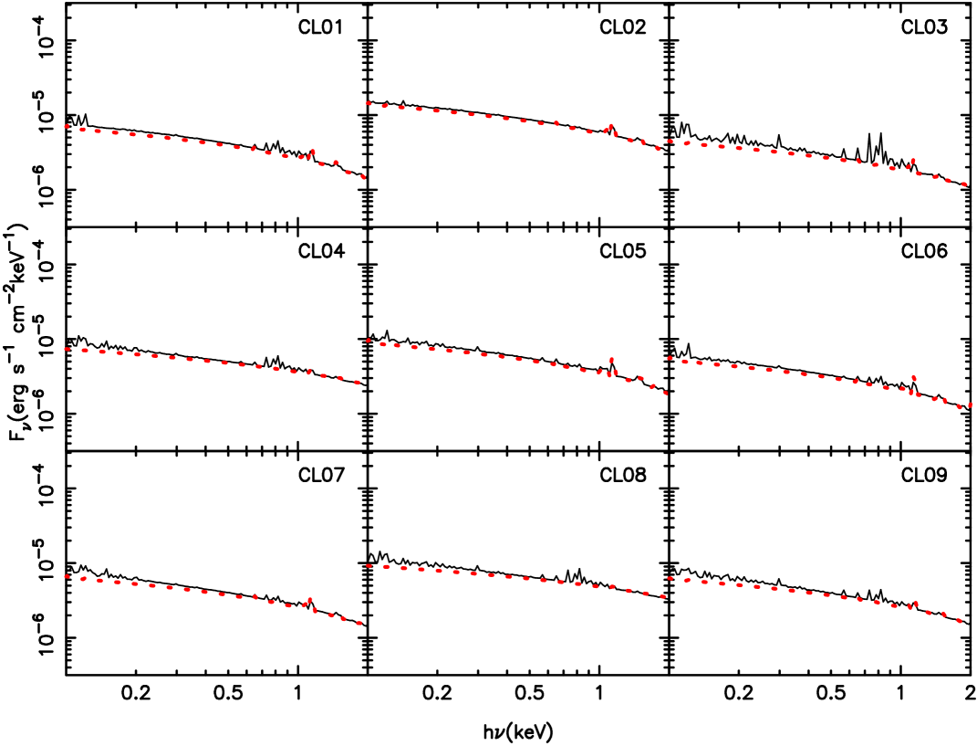
Figure 1: Simulated spectra as seen in the projected region within $0.4R_{\rm vir}$ from the cluster center, for a representative subset of 9 clusters (solid lines). The dotted lines are for the spectra expected from a one-temperature and one-metallicity plasma model, using the values of $T_{\rm ew}$ and $Z_{\rm ew}$ computed within the same region in the [1–2] keV energy band.

The result of this comparison is shown in Figure 1, where we plot the projected luminosity density as a function of the frequency, $F_{\nu}$, for cluster-centric distances $R\leq 0.4\,R_{\rm vir}$. Instead of showing spectra for the whole cluster set, we report here the results only for the first nine clusters of the list. The solid lines show the synthetic spectra, while the dotted lines are the prediction from the one–temperature and one–metallicity model. Quite apparently, the two spectra are always very similar, thus demonstrating that no appreciable soft excess is generated in the central regions of our simulated clusters. The only appreciable difference is related to the presence of soft metal lines in the synthetic spectra.

A quite different result is found if we concentrate, instead, on more external cluster regions, $0.4\leq R/R_{\rm vir}\leq 0.7$ (see Figure 2), which corresponds to the typical scales where the soft excess is detected from observational data. In this case, a fair number of clusters in our set shows evidence for a significant excess at $h\nu\raise-2.0pt\hbox{\hbox to0.0pt{\hbox{$\sim$}\hss}\raise 5.0pt\hbox{$<$}\ }1$ keV, thus witnessing the presence of a warm gas component, which contributes to the soft X–ray emission. This result is consistent with the observational evidence for a X–ray excess, that is more pronounced at larger cluster–centric radii (e.g., Bonamente et al. 2002; see the discussion here below).

In order to quantify the amount of soft excess, we define the relative excess

$$\eta=\frac{p-q}{q}$$ (4)

(see Bonamente et al. 2002), where $p$ is the flux in a given soft band, as computed from the synthetic spectrum, and $q$ is the prediction from the hot ICM model. We provide in Table 1 the values of the relative excess measured in this region, after projecting each cluster along three orthogonal directions. In about 30 per cent of the cases, we find a relative excess $\eta>0.5$. In several cases, the $\eta$ value for the same cluster changes quite substantially with the projection direction. This already indicates that the excess is sensitive to the occurrence of a few significant structures along the line-of-sight, rather than to the overall large–scale distribution of the gas.

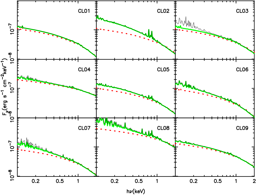
Figure 2: The same as in Figure 1, but in the 0.4–0.7 $R_{\rm vir}$ projected region. In addition the thick lines are the same as the thin lines, but using only the gas particles whose line-of-sight distance from the cluster centers is $\leq R_{\rm vir}$.

Having established that the soft excess phenomenon is rather common in the outskirt region of simulated clusters, when observed in projection, it is worth asking whether such an excess is generated by warm gas inside clusters or is associated to fore/back–ground large–scale filamentary structures, extending over scales of several Mpc. Large-scale hydrodynamic simulations (e.g. Cen & Ostriker 1999; Cen et al. 2001; Davé et al. 2001) indicate that about half of the baryons in the local Universe exist in the form of a warm-hot intergalactic medium (WHIM) with temperature $T\sim 10^{5}$–$10^{7}K$. The WHIM permeates the so-far elusive large–scale filamentary structures, from which galaxy clusters continuously accrete gas. Therefore, it is quite possible that the soft excess originates from large–scale diffuse filaments. On the other hand, an observational census of the baryons inside clusters (Ettori 2003) suggests that about 20 per cent of the ICM may be contributed by warm gas in the above temperature range. This gas would also provide a soft X–ray emissivity on top of that generated by the hot gas heated to the cluster virial temperature.

Tracing in simulations the gas distribution in the large–scale environment of galaxy clusters offers the possibility to distinguish between the internal and the external origin for the soft excess. To this purpose, we compute the synthetic spectrum of each cluster by excluding from the observational cylinder all the gas particles lying at a distance larger than $R_{\rm vir}$ along the line-of-sight from the cluster center. The corresponding spectra are shown with the thick lines in Figure 2. In the large majority of the cases we find that, after excluding the contribution from the gas outside $R_{\rm vir}$, the spectrum shows only a very modest change. This implies that the soft excess is mostly contributed by warm gas residing inside the virial cluster regions, while excluding a significant contribution from the large–scale filaments. The only exception, among the nine clusters shown in Fig. 2, is represented by CL03, for which a significant part of the excess is generated outside the virial region. A visual inspection of the gas distribution along the projection direction reveals the presence of a small group just approaching the virial region of the cluster, which is responsible for this excess.

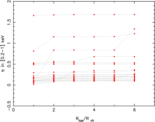
Figure 3: The relative excess $\eta$ in the [0.2-1] keV energy band, estimated in the region $0.4<R/R_{\rm vir}<0.7$, as a function of the maximum line-of-sight distance from the cluster center, $R_{\rm los}$. Here we show results for the 20 clusters projected only along one direction.

In order to investigate this point further, we show in Figure 3 how the relative excess changes with the extension along the line-of-sight, $R_{\rm los}$, of the region where the spectra are computed. In most cases the values of $\eta$ do not increase beyond $R_{\rm los}=R_{\rm vir}$, thus confirming that the excess does not generally receive a significant contribution outside the cluster virial regions. In the few cases where the excess increases along the line-of-sight, this takes place always in a narrow interval of distance. This confirms that the excess is contributed by individual small–scale structures (i.e. fore/background groups), rather than by the integrated effect of large–scale filaments.

In general, the amount of soft X–ray emission from filaments may depend on the energy feedback from SN and AGN, that heats the diffuse baryons: an efficient feedback brings the gas on a high adiabat, thus preventing it from reaching the density contrast of dark matter within filaments, therefore suppressing its X–ray emissivity. As discussed in Paper I, the feedback used in this simulation may be somewhat too weak to prevent overcooling within clusters and to break to the observed level the self–similarity of X-ray scaling relations at the scale of galaxy groups. If more efficient feedback needs to be introduced, then we expect an even smaller contribution of filaments to the soft X–ray excess.

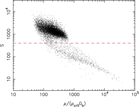
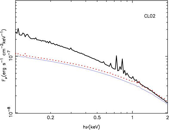
Figure 4: Tracing the gas particles responsible for the soft excess in the CL02 cluster. Left panel: the phase diagram shows entropy vs. density for the gas particles at projected cluster–centric distance $0.4<R/R_{\rm vir}<0.7$. Right panel: the synthetic spectrum of CL02 (thick line) is compared with that expected from the hot ICM one (dotted curve) and with the synthetic one obtained by excluding from the computations all the gas particles with entropy $S<400$ keV cm² (horizontal dashed line in the left panel).

In order to verify whether the soft excess is generated by a diffuse warm gas phase or by high density gas within subhalos, we plot in the left panel of Figure 4 the entropy–density phase diagram of the gas lying at projected cluster–centric distance $0.4<R/R_{\rm vir}<0.7$ for the CL02 cluster. This structure is the one displaying the largest excess among those shown in Fig.2. The entropy of the $i$–th gas particle is defined as $S_{i}=T_{i}/n_{e,i}^{2/3}$, where $T_{i}$ is its temperature (in keV) and $n_{e,i}$ is the associated number density of electrons (in cm^-3). Quite apparently, gas particles occupy two distinct regions of the $S$–$\rho$ plane; (1) the high–entropy low–density region, which corresponds to the shocked phase formed by gas whose high entropy has been generated by diffuse accretion; (2) a tail of condensed gas at lower entropy and high density, which is formed by gas within merging subhalos that preserved its low entropy during the accretion phase. As shown in the right panel of Fig. 4, the soft excess disappears once we remove the condensed gas phase (i.e., particles with $S<400$ keV cm²) from the computation of the spectrum. This demonstrates that the soft excess is associated with the presence of previously virialized clumps of high density gas at a temperature of a few tenths of keV, which are still surviving in the ICM, rather than to a diffuse phase of warm gas superimposed on the hot cluster atmosphere.

3.2 Comparison with observations

Using ROSAT–PSPC pointings of the Coma cluster, Bonamente et al. (2003) reported the detection of a soft excess in the [0.2–1] keV band at a high statistical significance. After performing the analysis at different angular distances from the cluster center, they concluded that the relative excess is an increasing function of this distance. In order to verify how typical is this result within our set of simulated clusters, we convert angular scales at the redshift of Coma to physical scales, and then rescale physical scales in units of the virial radius. To this purpose, we take the value, $R_{\rm vir}=1.9\,h^{-1}{\rm Mpc}$ obtained for the Coma cluster by Lokas & Mamon (2003) from their analysis of the kinematics of cluster galaxies. The result of this comparison is shown in Figure 5. Crosses are the observational values of the average excess within different annuli, as reported in Table 2 of Bonamente et al. (2003). For each of the 20 simulated clusters, we plot the excess obtained by projecting along three orthogonal directions. The solid line marks the upper 90 percentile in the distribution of the relative soft excesses in simulated clusters.

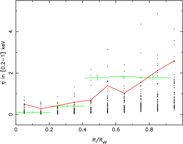
Figure 5: The relative excess $\eta$ in the [0.2-1] keV energy band, as a function of the projected cluster–centric distance, in units of the virial radius, from the simulated clusters (points), compared to the observational results for Coma (crosses with errorbars) as reported by Bonamente et al. (2003). With the exception of the outermost point, each observational point represents the average excess value computed over four quadrants, in which the Coma cluster has been divided. For each simulated cluster, we report the excess computed by projecting it along three orthogonal directions. The solid line shows the upper $90$ percentile for the distribution of the excess computed over the ensemble of simulated clusters.

As a general result, both simulations and observational data show a relative excess that increases with the projected radius. The lower soft excess at small radii is due to the less complex thermal structure of the ICM in the inner cluster regions: small sub–clumps reaching such regions had time to be disrupted and their gas to get thermalized with the surrounding hot cluster atmosphere. Still, for $0.4\raise-2.0pt\hbox{\hbox to0.0pt{\hbox{$\sim$}\hss}\raise 5.0pt\hbox{$<$}\ }R/R_{\rm vir}\raise-2.0pt\hbox{\hbox to0.0pt{\hbox{$\sim$}\hss}\raise 5.0pt\hbox{$<$}\ }0.7$, the excess observed in Coma is somewhat higher than the level of the 90 percentile in the distribution of the simulated soft X–ray excess. This indicates that an excess as large as that observed in the Coma cluster represents a rather rare event in our set of simulated clusters. We refrain from drawing any strong conclusion from this comparison, since most of the simulated clusters in our set are substantially smaller than the Coma cluster.

From their analysis of an ensemble of galaxy clusters, observed with the ROSAT–PSPC, Bonamente et al. (2002) report that the soft excess in the narrower [0.2–0.4] keV band is in fact a rather widespread phenomenon, which is detected at high significance in a fair fraction, $\sim 20$ per cent, of the sources. We compare in Figure 6 the relative excess in this band as a function of the cluster temperature, for both observed and simulated systems. As for data, the values of the excess are those reported in Figure 3 by Bonamente et al. (2002), while the temperature values have been taken from White (2000). The simulation results are obtained by computing the mean relative excess within $0.7\,R_{\rm vir}$, therefore including also the contribution from the innermost regions. This scale represents a good approximation to the typical size of the regions covered by observations. Within the temperature interval sampled by both observed and simulated clusters, the corresponding values of the relative excess are quite consistent with each other. We note that few observed systems have a significant negative excess. Bonamente et al. (2002) interpret this as due to a soft absorption associated to the presence of cold gas in central cluster regions. For $T\raise-2.0pt\hbox{\hbox to0.0pt{\hbox{$\sim$}\hss}\raise 5.0pt\hbox{$<$}\ }2$ keV the scatter in the relative excess increases for simulations, with few clusters being characterized by a soft X–ray excess larger than 20 per cent. This indicates that the relative importance of the warm component of the ICM increases in a few cases for colder systems, thus potentially leading to an intrinsic difficulty of defining a single temperature for systems with temperature below 2 keV (see also Mazzotta et al. 2004).

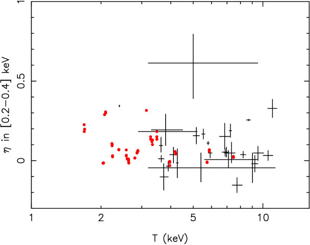
Figure 6: The relative excess $\eta$ in the [0.2-0.4] keV energy band for the observational data by Bonamente et al. (2002; crosses indicate the 1$\sigma$ uncertainties) and for simulations (filled circles). Results from simulations are obtained by computing the mean excess within $0.7\,R_{\rm vir}$, which represents a good approximation for the scales sampled by observations. As in Figure 5, we plot for each cluster the results obtained by projecting along three orthogonal directions.

As a concluding remark, it is worth mentioning that the approximate treatment of metal production in our simulation represents a potential source of uncertainty in the estimate of the soft excess. As already mentioned, the simulation includes energy feedback and the production of metals only from SN-II, using global metal yields (SH03). This is the main reason for the rather low metallicity measured in the simulated clusters (see Table 1). An improved treatment of the chemical enrichment of the gas in simulations requires accounting for the contribution from SN–Ia, hereby including detailed stellar yields and stellar evolution models (e.g., Tornatore et al. 2004, and references therein). As we have shown, the soft excess is associated to clumped gas at a temperature of a few tenths of keV. At such temperatures, a significant fraction of the emissivity is associated to metal lines. Therefore, an underestimate of the plasma metallicity would lead to an underestimate of the synthetic soft flux from the warm clumps, while leaving nearly unaffected the soft flux from the hot cluster atmosphere. In this respect, the values of the soft excess presented here may be somewhat underestimated.

4 Conclusions and future perspectives

We have studied a sample of 20 simulated clusters, extracted from a large SPH cosmological simulation of a concordance $\Lambda$CDM model, with the aim of exploring the presence and the origin of the soft X–ray excess in galaxy clusters. Besides the non–radiative gas dynamics, our simulation includes the treatment of star formation and energy feedback from galactic winds powered by supernovae. As such it provides a quite realistic description of the evolution of the diffuse gas in a cosmological environment.

Each cluster is observed in projection, by including the line-of-sight contribution from the surrounding large-scale gas distribution. This allows us to verify whether simulated clusters predict any soft excess of thermal origin and whether such an excess is generated within or outside the cluster virial region. Our analysis is aimed at mimicking the observational procedure followed by Bonamente et al. (2002, 2003), in their analysis of ROSAT–PSPC data. For each cluster we compute the corresponding emission–weighted temperature and metallicity in a relatively hard energy band. These values are then used to calculate the spectrum of a one-temperature and one-metallicity plasma model. The flux predicted by this spectrum in a softer band is then compared to that from the synthetic spectrum, computed by summing over the contribution of all the gas particles lying within the “observational cylinder” of each simulated cluster.

Our main results can be summarized as follows.

(a)

A significant soft X–ray excess is detected for cluster-centric distances $0.4<R/R_{\rm vir}<0.7$, whose amount varies from cluster to cluster (see Table 1 and Fig.2). In about 30 per cent of the cases we detect a relative excess at least as large as 50 per cent. However, the excess turns out to be always negligible in the central cluster regions, $R<0.4R_{\rm vir}$ (see Fig.1).

(b)

In most of the cases, the excess is found to originate inside the virial region of the simulated clusters (see Fig.3). In the few cases in which a sizable contribution to the excess arises from the large–scale cluster environment, we find that it is contributed by fore/background groups lying along the cluster line-of-sight. Based on this result, we predict that the soft excess detected in observations receives only a minor contribution from the warm–hot medium permeating the large–scale cosmic web.

(c)

Even within the virial cluster regions, the soft excess is contributed by high–density and low–entropy gas, rather than by a diffuse phase of warm gas (see Fig.4). This gas is associated to merging sub–groups, which still preserve their identity before being destroyed and thermalized in the hot ICM.

(d)

We compare our results with those reported by Bonamente et al. (2003) for the Coma cluster. Although both observations and simulations show that the relative excess increases with the cluster-centric distance, its value in Coma is larger than for most of the simulated clusters. This implies that an excess as large as that observed for Coma is a rather rare event in our set of simulated systems.

A general conclusion of our analysis is that a soft X–ray excess of thermal origin is naturally predicted by hydrodynamical simulations of galaxy clusters in a cosmological environment. While this is an interesting result per se, we believe that the comparison between data and simulation does not yet have the required level of accuracy to exclude the presence of a non–thermal origin (i.e., inverse Compton scattering), at least for part of the observed excess. There is little doubt that solving this issue requires both a more refined analysis of simulations and higher quality data.

Recent XMM–Newton observations have confirmed the presence of a soft excess in the Coma cluster (Finoguenov et al. 2003) and in other four clusters (Kaastra et al. 2003), which are consistent with having a thermal origin. Finoguenov et al. (2003) claims that the soft excess arises from a fairly large filamentary structure containing warm gas. Although this result may be in contradiction with our results from the simulations, it is clear that a detailed comparison would require mimicking the observational procedure as close as possible on a cluster-by-cluster basis.

It is clear that establishing the exact amount, nature and origin of the soft X–ray excess requires an optimal control of observational systematics, such as the instrumental calibration, accounting for instrumental and cosmic background, as well as for the galactic hydrogen column density in the cluster direction. Indeed, since the soft emission occurs close to the lower boundary of the useful energy range of currently available detectors, it is of paramount importance to assess the accuracy of their calibration.

On the other hand, a detailed analysis of simulations requires reproducing as close as possible the observational setup. In the analysis presented in this paper, synthetic spectra of the simulated clusters have been generated under the assumptions of dealing with an ideal detector, with a flat response function across the whole energy range of interest, and with no, or perfectly controlled, background. It is clear that, with the steadily increasing quality of data and level of sophistication of numerical simulations, accounting for the instrumental features is mandatory for a self–consistent and meaningful comparison between theoretical predictions and observations, with both operating (e.g., Gardini et al. 2003) and planned satellites (e.g., Yoshikawa et al. 2004). We are currently undertaking a program of simulation analysis, based on mimicking XMM–Newton spectrum observations with both pn and MOS detectors. This will allow us to perform a more quantitative comparison with observations, so as to shed light on the implication of the soft excess on the physical properties of baryons within and around galaxy clusters.

- (1) Anders, E.& Grevesse, N. 1989, GeCoA, 53, 197
- (2) Arnaud, M., et al. 2001,A&A, 365, L67
- (3) Baumgartner, W. H., Loewenstein, M., Horner, D. J., & Mushotzky R. F. 2003, ApJ, submitted (astro-ph/0309166)
- (4) Berghofer, T.W. & Bowyer, S. 2002, ApJ, 565, L17
- (5) Bonamente, M., Lieu, R. & Mittaz, J.P.D. 2001a, ApJ, 547, L7
- (6) Bonamente, M., Nevalainen, J., & Kaastra, J.S. 2001b,ApJ, 552, L7
- (7) Bonamente, M., Lieu, R., Joy, K.M. & Nevalainen, H.J. 2002 ApJ, 576, 688
- (8) Bonamente, M., Joy, K.M. & Lieu, R. 2003, ApJ, 585, 722
- (9) Borgani, S., Murante, G., Springel, V. et al. 2004, MNRAS, 348, 1078 (Paper I).
- (10) Bowyer, S., Berghofer, T.W. & Korpela, E.J. 1999, ApJ, 526, 592
- (11) Bregman,J. N., Dupke,R. A., Miller,E. D., 2004, ApJ, in press, astro-ph/0407365
- (12) Cen, R. & Ostriker, J. P. 1999, ApJ, 514, 1
- (13) Cen, R., Tripp, T., Ostriker, J. & Jenkins, E., 2001, ApJ, 559, L5
- (14) Davé, R., et al. 2001, ApJ, 552, 473
- (15) De Paolis, F., Ingrosso, G., Nucita, A.A. & Orlando, D. 2003, A&A, 398, 435
- (16) Durret, F., Slezak, E., Lieu, R., Dos Santos, S. & Bonamente, M. 2002, A&A, 390, 397
- (17) Eke, V. R., Cole, S., Frenk, C. S., & Navarro, J. F. 1996, MNRAS, 281,703
- (18) Enlin T. A., & Biermann, P. L. 1998, A&A, 330, 90
- (19) Ettori, S. 2003, MNRAS, 344, L13
- (20) Finoguenov, A., Briel,G. U., Henry, P. J. 2003, A&A, 410, 777
- (21) Gardini, A., Rasia, E., Mazzotta, P., et al. 2004, MNRAS, 351, 505
- (22) Hwang, C.-Y. 1997, Science, 278, 1917
- (23) Ikebe,Y., Reiprich, T.H., Böhringer, H., Tanaka, Y., & Kitayama, T. 2002, A&A, 383,773
- (24) Kaastra, J. S., Lieu, R., Tamura, T., Paerels, F. B. S.,& den Herder,J. W. 2003, A&A, 397, 445
- (25) Lieu, R., Mittaz,J.P.D., Bowyer, S. et al. 1996a, ApJ, 458, L5
- (26) Lieu, R., Mittaz,J.P.D., Bowyer, S. et al. 1996b, Science, 274, 1335-1338
- (27) Lokas, E. L.& Mamon, G. A. 2003, MNRAS, 343, L401
- (28) Maloney, P.R.,& Bland-Hawthorn, J. 2001,ApJ, 553, L129
- (29) Mathiesen, B. F. & Evrard, A. E. 2001, ApJ, 546, 100
- (30) Mazzotta, P., Rasia, E., Moscardini,L., & Tormen, G. 2004, MNRAS, in press (astro-ph/0404425)
- (31) Mittaz, J.P.D., Lieu, R., Lockman, F.J. 1998, ApJ, 498, L17
- (32) Nevalainen, J., Lieu, R., Bonamente, M., & Lumb, D. 2003,ApJ, 584, 716
- (33) Raymond, J.C.,& Smith, B.W. 1977, ApJS, 35, 419
- (34) Springel, V., Yoshida, N., White, S.D.M., 2001, NewA, 6, 79
- (35) Springel, V., Hernquist, L., 2002, MNRAS, 333, 649
- (36) Springel, V., Hernquist, L., 2003, MNRAS, 339, 289 (SH03)
- (37) Tornatore, L., Borgani, S., Matteucci, F., Recchi, S., &Tozzi, P. 2004, MNRAS, 349, L19
- (38) Yoshikawa, K., Dolag,K., Suto, Y. et al. 2004, PASJ, submitted (astro-ph/0408140)
- (39) White, D. A. 2000, MNRAS, 312, 663