CHEMICAL ABUNDANCES FOR SEVEN GIANT STARS IN M68 (NGC 4590) : A GLOBULAR CLUSTER WITH ABNORMAL SILICON AND TITANIUM ABUNDANCES

Abstract

We present a detailed chemical abundance study of seven giant stars in M68 including six red giants and one post-AGB star. We find significant differences in the gravities determined using photometry and those obtained from ionization balance, which suggests that non-LTE effects are important for these low-gravity, metal-poor stars. We adopt an iron abundance using photometric gravities and Fe II lines to minimize those effects, finding [Fe/H] = $-$2.16 $\pm$ 0.02 ($\sigma=0.04$). For element-to-iron ratios, we rely on neutral lines vs. Fe I and ionized lines vs. Fe II (except for [O/Fe]) to also minimize non-LTE effects.

We find variations in the abundances of sodium among the program stars. However, there is no correlation (or anti-correlation) with the oxygen abundances. Further, the post-AGB star has a normal (low) abundance of sodium. Both of these facts add further support to the idea that the variations seen among some light elements within individual globular clusters arises from primordial variations, and not from deep mixing.

M68, like M15, shows elevated abundances of silicon compared to other globular clusters and comparable metallicity field stars. But M68 deviates even more in showing a relative underabundance of titanium. We speculate that in M68, titanium is behaving like an iron-peak element rather than its more commonly observed adherence to enhancements seen in the “$\alpha$” elements such as magnesium, silicon, and calcium. We interpret this result as implying that the chemical enrichment seen in M68 may have arisen from contributions from supernovae with somewhat more massive progenitors than contribute normally to abundances seen in other globular clusters.

The neutron capture elements barium and europium vary among the stars in M15 (Sneden et al. 1997), but the [Ba/Eu] is relatively constant, suggesting that both elements arise in the same nucleosynthesis events. M68 shares the same [Ba/Eu] ratio as the stars in M15, but the average abundance ratio of these elements, and lanthanum, are lower in M68 relative to iron than in M15, implying a slightly weaker contribution of $r$-process nucleosynthesis in M68.

1 INTRODUCTION

Globular clusters in our Galaxy do not define a single homogeneous population with a single history. In his pioneering work, Zinn (1985) subdivided the globular clusters into the “halo” and the “thick disk” groups at [Fe/H] = $-$0.8. The halo clusters have an essentially spherical distribution about the Galactic center and they constitute a pressure supported system (a small rotational velocity and a larger velocity dispersion), while the thick disk clusters have a highly flattened spatial distribution and constitute a rotational supported system (a larger rotational velocity and a smaller velocity dispersion). Searle & Zinn (1978) and Lee, Demarque, & Zinn (1994) suggested that the inner halo globular clusters exhibit a tight horizontal branch (HB) morphology versus [Fe/H] relation, while the outer halo globular clusters show the second parameter phenomenon (i.e., a larger scatter in HB type at a given [Fe/H]). Subsequently, Zinn (1993) subdivided the halo clusters into two groups. The “old halo” group obeys the same HB type versus [Fe/H] relationship as the inner halo clusters while the “younger halo” group deviates from this relationship by a significant amount (see Figure 1). Zinn (1993) and Da Costa & Armandroff (1995) argued that the old and the younger halo groups have different kinematic properties that the old halo group has a prograde mean rotation velocity with a smaller velocity dispersion while the younger halo group has a retrograde mean rotation velocity about the Galactic center with a larger velocity dispersion. They suggested that the old halo group formed during the collapse that led ultimately to the formation of the Galactic disk and the younger halo group were accreted later in time. If so, one would expect to see signatures of different chemical enrichment history carved in spectra of stars in globular clusters. For example, one might be able to investigate the early form of the initial mass function (IMF) by studying abundances of stellar mass-sensitive elements (see discussion and references in McWilliam 1997).

An alternative perspective on “younger halo” and “old halo” clusters is that of dissolved and accreted dwarf galaxies. For example, Freeman (1993) suggested that the massive and chemically unusual globular cluster $\omega$ Cen might be the remnant nucleus of an accreted dwarf galaxy. Lynden-Bell & Lynden-Bell (1995) noted the possible alignments of orbital poles of some globular clusters such that they might comprise a “spoor” (more commonly referred to as a stream) of clusters. While the specific details have not found support, the idea has been demonstrated very nicely by Dinescu et al. (2000), who found a clear dynamical relationship between the space motions of the young globular cluster Palomar 12 and the Sagittarius dwarf galaxy. Indeed, other globular clusters may also be associated with this particular accretion event (NGC 5634: Bellazzini, Ferraro, & Ibata 2002; NGC 4147: Bellazzini et al. 2003; Palomar 2: Majewski et al. 2004). Yoon & Lee (2002) have similarly speculated on a dynamical relationship between some metal-poor globular clusters, including M68. Yoon & Lee (2002) suggested that M68 was a member of a satellite galaxy and accreted later in time to our Galaxy, resulting in a planar motion of several metal-poor clusters including M15 and M92.

Dynamical evolution in the Galaxy can eventually dissolve streams, making their detection difficult. However, an interesting alternative exists, called “chemical tagging”. As Freeman & Bland-Hawthorn (2002) discussed, stars born in galaxies whose star formation histories differ from those that have created the bulk of the Galaxy’s stars may still be discernible in unusual element-to-iron ratios. Indeed, Cohen (2004) has found a compelling link between Palomar 12 and the Sagittarius dwarf. Detailed chemical abundances of globular clusters may yet become the principle means of identifying historical links between stars and clusters that are now widely dispersed in our Galaxy.

M68 (NGC 4590) is part of the younger halo, according to its HB type with respect to its metallicity, and is located 10 kpc from the Galactic center. Dinescu, Girard, & van Altena (1999) have found that the cluster’s Galactic orbit carries it rather far from the Galactic center, perhaps as far as 30 kpc. As shown in Figure 1, globular clusters with [Fe/H] $\leq$ $-$2.0 have HB types that are greater than 0.6 with the exception of M68. If age is the second parameter, M68 represents the low metallicity tail of the younger halo globular clusters. The absolute age of M68 does appears to be slightly younger than those of the oldest globular clusters in our Galaxy. Rosenberg et al. (1999) argued that M68 is coeval to or slightly younger than those of the oldest halo globular clusters while VandenBerg (2000) discussed that the age of M68 is less than that of M92, one of the oldest globular clusters in our Galaxy, by $\approx$ 15%.

The previous metallicity estimates of M68 as follows. Zinn & West (1984) and Zinn (1985) adopted [Fe/H] = $-$2.09. Gratton & Ortolani (1989) observed two stars in M68 with one being in common with this study. They derived elemental abundances for 11 species including iron, finding [Fe/H] = $-$1.92. However, due to the low resolving power ($R$ = 15,000) of their spectra, their equivalent width measurements were vulnerable to line blending. Minniti et al. (1993) observed two stars in M68, one being in common with Gratton & Ortolani (1989) and this study, finding [Fe/H] = $-$2.17. Minniti et al. (1996) also discussed oxygen and sodium abundances of the cluster. Finally, Rutledge (1997) observed the infrared Ca II triplet for 19 stars and obtained [Fe/H] = $-$2.11 $\pm$ 0.03 using the Zinn & West (1984) [Fe/H] scale.

In this paper, we explore the detailed elemental abundances for seven giant stars in M68. One of these stars is a probable asymptotic giant branch (AGB) stars and the remaining six are red giant branch (RGB) stars. This study is tied directly to that of Lee & Carney (2002) with the same instrument setups and analysis methods.

2 OBSERVATIONS AND DATA REDUCTION

The observations were carried out from 4 to 7 May 1996. We selected our program RGB stars from the $BV$ photometry of Walker (1994). The positions of our target giant stars on the color-magnitude diagram along with bright stars in M68 are shown in Figure 2. In Table 1, we provide identifications (Alcaino 1977; Harris 1975; Walker 1994), position (Cutri et al. 2000), $V$ magnitudes, $(B-V)$ colors (Walker 1994) and $K$ magnitudes (Frogel, Persson, & Cohen 1983; Cutri et al. 2000) of our target stars. Please note that the 2MASS $K$ magnitudes have been converted to the CIT system (Cutri et al. 2000) are in good agreement with those of Frogel et al. (1983). We obtained high signal-to-noise ratio (S/N $\geq$ 90 per pixel) echelle spectra using the CTIO 4-meter telescope and its Cassegrain echelle spectrograph. The Tek 2048 $\times$ 2048 CCD, 31.6 lines/mm echelle grating, long red camera, and G181 cross-disperser were employed for our observations. The slit width was 150 $\mu$m, or about 1.0 arcsec, that projected to 2.0 pixels and which yielded an effective resolving power $R$ = 28,000. Each spectrum had complete spectral coverage from 5420 to 7840 Å. All program star observations were accompanied by flat lamp, Th-Ar lamp, and bias frames.

The raw data frames were trimmed, bias-corrected, and flat-fielded using the IRAF ARED and CCDRED packages. The scattered light was also subtracted using the APSCATTER task in ECHELLE package. The echelle apertures were then extracted to form 1-d spectra, which were continuum-fitted and normalized, and a wavelength solution was applied following the standard IRAF echelle reduction routines.

Equivalent widths were measured mainly by the direct integration of each line profile using the SPLOT task in IRAF ECHELLE package. We estimate our measurement error in equivalent width to be $\pm$2 mÅ from the size of noise features in the spectra and our ability to determine the proper continuum level. The equivalent widths for our program stars are listed in Table 2.

Gratton & Ortolani (1989) and Minniti et al. (1993) obtained a spectrum of one star in common with our program stars. They used the identifications from Harris (1975) while we have used those of Walker (1994). Comparing the two shows that the star I-260 from Harris (1975) is the same as the star 160 from Walker (1994). Figure 3 compares equivalent width measurements of our work with those measured by Gratton & Ortolani (1989; crosses) and Minniti et al. (1993; open circles). The agreement with the latter study is quite good, with a mean difference of $2.3\pm 1.5$ mÅ (in the sense of their study minus ours). The instrumental resolving powers for the two studies were very similar (27,000 vs. 28,000). However, the lower resolving power of the observations reported by Gratton & Ortolani (1989), about 15,000, appears to have led to systematically larger equivalent widths, as Figure 3 reveals. The mean difference is $13.8\pm 2.7$ mÅ.

3 ANALYSIS

In our elemental abundance analysis, we use the usual spectroscopic notations that $[A/B]\equiv\log(N_{A}/N_{B})_{star}-\log(N_{A}/N_{B})_{\sun}$, and that $\log n(A)\equiv\log(N_{A}/N_{H})+12.00$ for each element. For the absolute solar iron abundance, we adopt $\log n$(Fe) = 7.52 following the discussion of Sneden et al. (1991).

3.1 Line Selection and Oscillator Strengths

For our line selection, laboratory oscillator strengths were adopted whenever possible, with supplemental solar oscillator strength values. In addition to oscillator strengths, taking into account the damping broadening due to the van der Waals force, we adopted the Unsöld approximation with no enhancement.

The abundance analysis depends mainly on the reliability of the oscillator strength values of the Fe I and Fe II lines, since not only the metallicity scale but also the stellar parameters, including the spectroscopic temperature, surface gravity, and microturbulent velocity, will be determined using these lines. As discussed by Lee & Carney (2002), we mainly relied upon the extensive laboratory oscillator strength measurements by the Oxford group (Blackwell et al.  1982b, 1982c, 1986a). We also used oscillator strength values measured by O’Brian et al. (1991) and the Hannover group (Bard, Kock, & Kock 1991; Bard & Kock 1994). In our iron abundance analysis, we consider the Oxford group’s measurements (the absorption method) as the “primary” oscillator strengths and oscillator strength measurements that relied on emission methods (O’Brian et al. 1991; Bard, Kock, & Kock 1991; Bard & Kock 1994) as “secondary”. Therefore, the oscillator strengths by O’Brian et al. and the Hannover group were scaled with respect to those by the Oxford group as a function of excitation potential (de Almeida 2000, private communication),

$$\log gf = \log gf(OB)-0.017,$$

$$\log gf = \log gf(H91)-0.015-0.009\chi,$$

$$\log gf = \log gf(H94)-0.027-0.009\chi,$$ (1)

where the excitation potential $\chi$ is given in electron volts. Blackwell, Smith, & Lynas-Gray (1995) also pointed out that there appears to exist a slight gradient in the excitation potential between oscillator strengths by the Oxford group and those by the Hannover group, with $\log gf(Oxford)=\log gf(Hannover)-0.021-0.006\chi$.

For neutral titanium lines, we relied on the laboratory measurements by the Oxford group (Blackwell et al. 1982a, 1983, 1986b). It should be noted that the original Oxford $gf$-values have been increased by +0.056 dex following Grevesse, Blackwell, & Petford (1989). They discussed that the Oxford $gf$-values relied on the inaccurate lifetime measurements and the absolute $gf$-values should be revised based on the new measurements.

Hyperfine splitting (HFS) components must be considered in the barium abundance analysis because Ba II lines are usually very strong even in metal-poor stars and the desaturation effects due to HFS components become evident (see for example, McWilliam 1998). We adopted the Ba II HFS components and oscillator strengths of Sneden et al. (1997). We also perform HFS treatment for scandium, manganese (Prochaska & McWilliam 2000) and copper (Kurucz 1993). For the copper HFS analysis, we adopt the solar Cu isotopic ratio, 69% ⁶³Cu and 31% ⁶⁵Cu, following the discussions given by Smith et al. (2000) and Simmerer et al. (2003). The equivalent widths of Mn I $\lambda$ 6021.79 Å and Cu I $\lambda$ 5782.13 Å lines in our program stars are weak and the Mn and Cu abundance differences between HFS treatment and non-HFS treatment are no larger than 0.02 dex. We list our source of oscillator strengths for each element in Table 3.

3.2 Stellar Parameters and Model Atmospheres

Having good stellar parameters, such as the effective temperature and the surface gravity, is critical for any stellar abundance study, since the absolute or the relative elemental abundance scale will depend on the input stellar parameters. For our analysis, we rely on spectroscopic temperatures and photometric surface gravities, following the method described in Lee & Carney (2002; see also Ivans et al. 2001, Kraft & Ivans 2003, and Sneden et al. 2004). It has been suspected by others that the traditional spectroscopic surface gravity determination method which requires the same elemental abundances derived from neutral and singly ionized lines (preferentially Fe I and Fe II lines) suffers from non-local thermodynamic equilibrium (NLTE) effects (see, for example, Nissen et al. 1997; Allende Prieto et al. 1999). Since metal-poor stars have much weaker metal-absorption in the ultraviolet, more non-local UV flux can penetrate from the deeper layers. This flux is vital in determining the ionization equilibrium of the atoms, resulting in deviations from local thermodynamic equilibrium (LTE). Nissen et al. (1997) claimed that surface gravities of metal-poor dwarfs and subgiants derived from the spectroscopic method, which demands that Fe I and Fe II lines should provide the same iron abundance, are a factor of two or three ($\Delta\log g\approx$ 0.3 – 0.5) smaller than those from the Hipparcos parallaxes. Allende Prieto et al. (1999) also claimed that spectroscopic gravities and those from the Hipparcos parallaxes are in good agreement for stars in the metallicity range $-1.0<$ [Fe/H] $<$ +0.3, while large discrepancies can be found for stars with metallicities below [Fe/H] = $-$1.0, in the sense that the spectroscopic method provides lower surface gravities. Therefore, we rely on photometric gravities for our abundance analysis.

The initial estimates of the temperature of program stars were estimated using $BVK$ photometry of our program stars (Cutri et al. 2000; Frogel, Persson, & Cohen 1983; Walker 1994) and the empirical color-temperature relations given by Alonso, Arribas, & Martinez-Roger (1999). Since their relation depends slightly on the metallicity, we adopted [Fe/H] = $-$2.1 for M68 (Harris 1996). To estimate the dereddened color, we adopt $E(B-V)$ = 0.07 (Walker 1994). Note that Alonso et al. (1999) employed the Carlos Sánchez Telescope (TCS) system for their infrared color-temperature relations and we used the relation given by Alonso, Arribas, & Martinez-Roger (1998) to convert the CIT system to the TCS system for $K$ magnitudes listed in Table 1. To derive photometric surface gravity in relation to that of the Sun, we use $\log g_{\sun}$ = 4.44 in cgs units, $M_{\rm bol,\sun}$ = 4.74 mag, and $T_{\rm eff,\sun}$ = 5777 K for the Sun (Livingston 1999) and we assume the stellar masses for all the red giants stars in this analysis to be $M$ = 0.8 $M_{\sun}$. We use the empirical relation given by Alonso et al. (1999) to estimate the bolometric correction and we adopt $(m-M)_{0}$ = 14.97 mag for the cluster (Harris 1996).

With initial photometric temperature and surface gravity estimates, 72-depth plane-parallel LTE model atmospheres were computed using the program ATLAS9, written and supplied by Dr. R. L. Kurucz. Assuming that all of the cluster’s stars would prove to be metal-poor, the model atmospheres were computed using opacity distribution functions and abundances with enhanced abundances of all the “$\alpha$” elements (O, Ne, Mg, Si, S, Ar, Ca, and Ti) by 0.4 dex. The “$\alpha$” element enhancements are important since several of these elements are quite abundant and are major electron donors to the H^- opacity. During our model computation, convective overshoot was turned off.

The abundance analysis was performed using the current version (2002) of the LTE line analysis program MOOG (Sneden 1973). Adopting the photometric temperature and surface gravity as our initial values, we began by restricting the analysis to those Fe I lines with $\log$(W_λ/$\lambda$) $\leq$ $-5.2$ (i.e., for the linear part of the curve of growth), and comparing the abundances as a function of excitation potential. New model atmospheres were computed with a slightly different effective temperature until the slope of the log n(Fe I) versus excitation potential relation was zero to within the uncertainties. The stronger Fe I lines were then added and the microturbulent velocity $v_{\rm turb}$ altered until the $\log$ n(Fe I) versus $\log$(W_λ/$\lambda$) relation had no discernible slope.

Table 4 shows our temperature and surface gravity of program stars. In the fifth column of the Table, we also show the temperature of five stars in common given by Frogel et al. (1983). Please note that Gratton & Ortolani relied on temperatures given by Frogel et al. (1983), which are 159 $\pm$ 27 K higher than our spectroscopic temperatures. The temperature difference between those derived from $(B-V)$ colors (column 2) and spectroscopic temperatures of this study is 72 $\pm$ 15 K (7 stars), in the sense that our spectroscopic temperature is low. The temperature difference between those derived from $(V-K)$ colors using $K$ magnitudes of Frogel et al. (column 3) and spectroscopic temperatures of this study is 54 $\pm$ 17 K (5 stars) and those derived from $(V-K)$ colors using 2MASS $K$ magnitudes (column 4) and spectroscopic temperatures of this study is 69 $\pm$ 14 K (7 stars). The discrepancy between photometric and spectroscopic temperatures from $(V-K)$ colors is slightly smaller than that from $(B-V)$ colors.

4 RESULTS

4.1 Elemental Abundances and Error Analysis

In Tables 5, we present the elemental abundances of our program stars using photometric surface gravities and spectroscopic temperatures. The [el/Fe] ratios for neutral elements are estimated from [el/H] and [Fe I/H] ratios, with the exception of oxygen. The [el/Fe] for singly ionized elements (Ti II, Ba II, La II, and Eu II) and oxygen are estimated from [el/H] and [Fe II/H] ratios (see, for example, Ivans et al. 2001, Kraft & Ivans 2003, Sneden et al. 2004). The internal uncertainty quoted is for a single line and, therefore, that of each element is given by $\sigma/\sqrt{n}$, where $\sigma$ is the uncertainty per line and $n$ is the number of absorption lines used for each element. Systematic errors, such as in adopted $gf$ values as a function of excitation potential, which could lead to systematically erroneous temperature estimates, are not included. The last two columns of the Table show the mean values of each element of the cluster with and without the star 117 (ZNG2), an ultraviolet-bright, post-AGB star according to Zinn, Newell, & Gibson (1972). We adopt iron abundances based only on the Fe II lines for our program stars since the Fe II abundance is thought to be less sensitive to NLTE conditions (see for example, Thévenin & Idiart 1999, Kraft & Ivans 2003). In Figure 4, we show abundances of all elements measured in this study against $T_{\rm eff}$, showing no discernible gradient in elemental abundances with $T_{\rm eff}$. The mean [Fe/H] of $-$2.16 dex for our seven stars is measured with a small internal uncertainty of $\pm$0.02 ($\sigma$ = 0.04).

For comparison, we also show the elemental abundances of our program stars using the traditional spectroscopic surface gravities (see column 7 of Table 4). In the Table, the [el/Fe] ratios are derived from [el/H] and mean [Fe/H] ratios. In Table 7, we show differences in elemental abundances using photometric and spectroscopic gravities. The [Fe/H] ratio using spectroscopic gravities is 0.25 dex lower than that using photometric gravities. For other elements, however, the elemental abundances from two different methods are in good agreement to within 0.10 dex. Therefore, these small differences suggest that we are still able, in principle, to compare our elemental abundances with other results using the different surface gravity determination method. Nonetheless, we reiterate that we choose to employ photometric gravities and will discuss only the results from Table 5.

In Table 8, we show estimated errors resulting from uncertainties in the input model atmosphere $\delta T_{\rm eff}$ = $\pm$ 80 K, $\delta\log g$ = $\pm$0.3 and $\delta v_{\rm turb}$ = $\pm$0.2 km s^-1, which are appropriate for our analysis. The Fe, Si, Ba, and La abundances are sensitive to $T_{\rm eff}$ resulting in $\mid$$\delta$[el/Fe (or H for Fe)]/$\delta T_{\rm eff}$(80 K)$\mid$ $\approx$ 0.08 – 0.12 dex. The iron abundance from Fe II lines is sensitive to surface gravity, $\mid$$\delta$[Fe II/H]/$\delta\log g$(0.3 dex)$\mid$ $\approx$ 0.10 dex. Since our program stars are metal-poor, absorption lines are usually weak as listed in Table 2. Therefore, our derived elemental abundances are less sensitive to the microturbulent velocity. The barium abundance is the most sensitive to the microturbulent velocity resulting in $\mid$$\delta$[Ba/Fe]/$\delta v_{\rm turb}$(0.2 km s^-1)$\mid$ $\approx$ 0.09 dex.

4.2 Comparisons with previous results

As mentioned above, Gratton & Ortolani (1989) and Minniti et al. (1993, 1996) derived abundances for star 160 (I-260 from Harris 1975). In Table 9, we compare our stellar parameters and elemental abundances of this star with those of Gratton & Ortolani (1989) and Minniti et al. (1993, 1996).

Gratton & Ortolani (1989) relied on the results from Frogel et al. (1983) for the estimated temperature and surface gravity. Table 4 shows that this results in a $T_{\rm eff}$ estimate 230 K hotter than our spectroscopic measurement, and a slightly lower microturbulent velocity (by 0.2 km s^-1) as well. Our results suggest that a difference in microturbulent velocity of 0.2 km s^-1 does not alter the derived iron abundances and element-to-iron ratios by more than about 0.1 dex. As discussed above (see also Figure 3), the equivalent widths measured by Gratton & Ortolani are about 14 mÅ larger than our measurements. This was also noticed by Minniti et al. (1993), who found a difference in equivalent width of 10.2 $\pm$ 9.0 mÅ, in the sense of Gratton & Ortolani minus Minniti et al. Therefore, the larger equivalent widths with the warmer surface temperature are the probable cause of the higher [Fe/H] value they derived. Therefore, the detailed comparison of each elemental abundance between this study and Gratton & Ortolani may not be meaningful.

Minniti et al. (1993) derived an even higher temperature of the star, $T_{\rm eff}$ = 4400 K, which is 300 K warmer than our temperature, and, consequently, their iron abundance of the star from Fe I lines is about 0.45 dex higher than our value, but, interestingly, very close to the value we obtain using only the Fe II lines. Minniti et al. (1993) obtained $\log g$ = 1.0 for the star, using the ionization equilibrium of iron lines, which is about 0.3 dex larger than those of Gratton & Ortolani (1989) and this study. This is very worrisome, since Minniti et al. (1993) used the same temperature determination method, the same model atmospheres as this study and similar oscillator strength values. Their instrumental resolution was comparable to ours, and they employed the program WIDTH rather than MOOG, but both programs yield the same results, in our experience, at least when the atomic data are identical. The equivalent widths are also in good agreement, as noted earlier. In particular, the agreement in the equivalent widths of weak lines (i.e., the lines on the linear part of the curve of growth) appears to be excellent. For lines with $\log$(W_λ/$\lambda$) $\leq$ $-5.2$, the difference in equivalent widths is $-$1.7 $\pm$ 1.4 mÅ (7 lines), in the sense of Minniti et al. minus this study.

Instead of comparing our results to those of Minniti et al. (1993) directly, we have rederived the surface temperature using the equivalent widths measured by Minniti et al. (1993). In their Table 2, Minniti et al. (1993) presented Fe I and Fe II line widths of the star 160. Using their Fe I line widths with $\log$(W_λ/$\lambda$) $\leq$ $-5.2$, we ran MOOG for this star again. At this time, we use a Kurucz model atmosphere with $T_{\rm eff}$ = 4400 K, $\log g$ = 1.0, and $v_{\rm turb}$ = 2.0 km s^-1 as our initial input model. Note that these stellar parameters are derived by Minniti et al. for their analyses of the star as shown in Table 9. We show the results from our MOOG run in Figure 5a. We obtain [Fe/H] = $-$2.18 $\pm$ 0.29 (36 lines) and this value is very similar to that of Minniti et al., [Fe/H] = $-$2.11. As can be seen in the Figure, however, the scatter in our analysis using the line list of Minniti et al. is much larger than that Minniti et al. estimated ($\sigma$ $\leq$ 0.07 dex per line) and we were not able to reproduce their results using their input data. We find it necessary to adopt a different temperature. Since the Fe I line at $\lambda$ 6353.84Å deviates far from the mean value of the relation, we excluded this line and ran MOOG again with $T_{\rm eff}$ = 4275 K and obtain [Fe/H] = $-$2.30 $\pm$ 0.22 dex (Figure 5b). For comparison, we show the results from MOOG run with our stellar parameters, $T_{\rm eff}$ = 4100 K, $\log g$ = 0.7, and $v_{\rm turb}$ = 1.8 km s^-1 in Figure 5c. We obtain [Fe/H] = $-$2.50 $\pm$ 0.13. In the Figure, the agreement between results from our equivalent widths and those of Minniti et al. for lines with $\chi$ $\leq$ 3 eV is good. For lines with $\chi$ $>$ 3 eV, the scatter in results from Minniti et al. is rather large. It is likely that the Fe I lines employed by Minniti et al. may have been contaminated, and as a result they would have obtained a higher iron abundance than we have. Their accidental inclusion of Fe I lines suffering from line blending made their measurements to meet the ionization equilibrium at high surface gravity $\log~{}g$ = 1.0. Using our line width measurements listed in Table 2, the criterion of the ionization equilibrium of iron lines is not satisfied until the surface gravity becomes as low as $\log~{}g$ = 0.0 and this surface gravity value is not only 1 dex smaller than that of Minniti et al., but is implausible.

We conclude that we do not understand why we cannot obtain the same results as did Minniti et al. (1993) using their data, and we conclude that the agreement between their [Fe/H] result and ours is probably fortuitous.

5 DISCUSSION

In the previous section, we discussed the rationale by which we have derived elemental abundance estimates. From the ionized iron lines, we obtain [Fe/H] = $-$2.16 $\pm$ 0.02 ($\sigma=0.04$) for M68 (based on internal errors only). Element-to-iron ratios are matched using comparable ionization states (except for oxygen, given its very high ionization potential).

We explore the abundances of a variety of elements relative to iron. In the interests of economy and of interest, we focus on comparisons between M68 and the comparably metal-poor globular cluster M15, based on the results of Sneden et al. (1997, 2000), and then discuss these in turn compared to other ensembles of field stars and clusters. We select M15 because it is one of the few metal-poor globular clusters with comparable data for the neutron capture elements lanthanum, barium, and europium, and partly because of the hypothesized common origin (Yoon & Lee 2002).

5.1 Mixing or Primordial Variations? O, Na, Mg, Al

Many globular clusters appear to show anticorrelations between the abundances of oxygen and sodium, and of magnesium and aluminum. The subject was reviewed by Kraft (1994), and has been revisited by numerous authors. The approach often taken has been that these anticorrelations arise from deep mixing, whereby material whose chemical compositions have been altered by proton captures within the CNO cycle have been brought to the stellar surface. This concept has become less plausible with the discovery that such anticorrelations are seen in relatively unevolved stars in the metal-poor clusters NGC 6397 and NGC 6752 (Gratton et al. 2001) and in the metal-rich cluster 47 Tuc (Carretta et al. 2004). The variations seen in some of these elements in Table 5 nonetheless warrant a quick look at these possible anti-correlations in M68, and we show them here in Figure 6, in comparison with the results for M15 from Sneden et al. (1997).

There are three relatively interesting results here. First is that M68 does show a variation, especially in sodium. The second is that the large range in sodium abundances is not matched by a correlated (or anti-correlated) variation in the oxygen abundances, as appears to be the case for M15. Finally, the post-AGB star 117, indicated by an open square in the Figure, is consistent with no signs of deep mixing, despite it clearly being the most evolved star in our study. The lack of an anti-correlation and the lack of variations seen in star 117 are consistent with a primordial variation for the differences in elemental abundances, presumably due to pollution during the earliest stages of the cluster formation and evolution by AGB nucleosynthesis and mass loss.

5.2 The Other Light Elements: Si, Ca, and Ti Abundances

Table 5 shows that the other light elements, silicon, calcium, and titanium, do not show any detectable variation in their abundances. These elements are of considerable interest nonetheless because they provide us with an opportunity to compare the nucleosynthesis histories of clusters, and, in principle, a means to compare the rate of star formation and, possibly, relative ages.

If star formation began everywhere in the Galaxy at about the same time, then the abundances of elements that emerge from Type II supernovae, including these light elements and $r$-process elements such as europium, will be enhanced relative to the abundances of elements that emerge from nucleosynthesis sites that appear more gradually, including $s$-process elements from AGB stars, and iron-peak elements from Type Ia supernovae. The details are complex, but this basic picture is consistent with the basic behavior of these “$\alpha$” elements’ abundances (see the discussions of Wyse & Gilmore 1988; Wheeler et al. 1989, and Carney 1996). If we compute unweighted averages for silicon, calcium, and titanium, we find for M68 that [$\alpha$/Fe] = $+0.34\pm 0.22$, which is roughly consistent with that found in M15 and other globular clusters. In Table 10, we summarize the [Si/Fe], [Ca/Fe], [Ti/Fe], and the mean [$\alpha$/Fe] ratios of M68, other globular clusters (Gratton 1987; Gratton & Ortolani 1989; Kraft et al. 1992, 1995, 1997, 1998; McWilliam et al. 1992; Sneden et al. 1994, 1997, 2000b; Brown et al. 1997, 1999; Ivans et al. 1999; Shetrone & Keane 2000) and field stars with $-2.50\leq$ [Fe/H] $\leq\ -1.90$ studied by Fulbright (2000). (The errors are those of the mean.) In the Table, old inner halo clusters denote metal-poor inner halo clusters NGC 6287 ([Fe/H] = $-$2.01), NGC 6293 ($-$1.99), and NGC 6541 ($-$1.76) and their Galactocentric distances are 1.6 kpc, 1.4 kpc, and 2.2 kpc, respectively (Lee & Carney 2002). The mean values of [$\alpha$/Fe] do not appear to vary much, and are probably consistent within the internal errors (the simple averages) and any lingering systematic errors.

A closer examination of the abundances of these elements does reveal some interesting differences, however. The silicon abundance of M68 appears to be similar to that found in M15, and both are enhanced relative to those of other clusters and field stars.

The calcium abundance of M68 is likewise similar to those found in M15, and both are similar to other halo stars and clusters. There may, however, be a modest difference ($\approx$ 0.15 dex) between M68, M15, and other “old halo” clusters and “younger halo” and thick disk clusters. Note that this contradicts the assignment of M68 to the “younger halo” category.

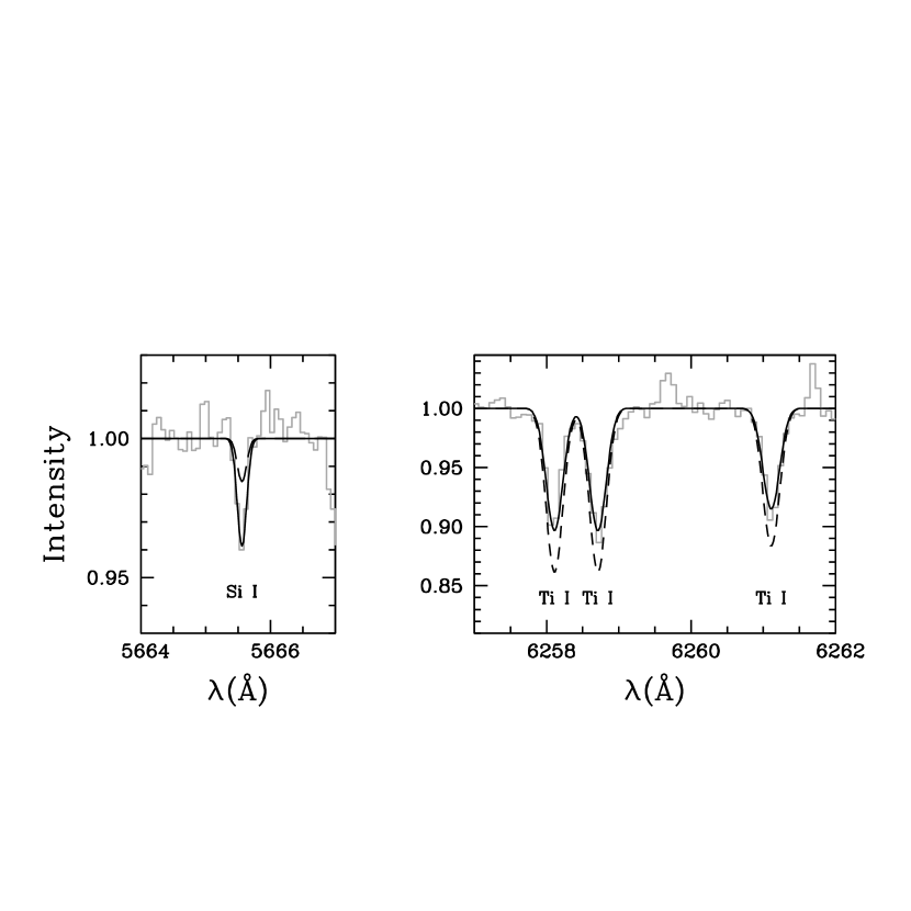
Figure 7: Comparisons of observed spectrum of the star M68-93 with those of synthetic spectra near Si I $\lambda$ 5665.56Å and Ti I $\lambda$ 6258.11, 6258.71, and 6261.11Å. The observed spectrum is presented by histograms, synthetic spectra with [Si/Fe] = +0.68, [Ti/Fe] = +0.06 by solid lines (see also Table 5), and synthetic spectra with [Si/Fe] = +0.30, [Ti/Fe] = +0.30 by dotted lines.

On the other hand, the titanium abundance of M68 appears to be much lower than all other clusters. Is this effect real? The titanium abundance of the metal-poor RGB stars using the neutral titanium lines may suffer from NLTE effects, such as an over-ionization, and the resultant Ti abundance may be spurious. However, our Ti abundance analyses using the Ti II lines also yield a lower titanium abundance for our program stars, indicating that they are truly titanium deficient. In Figure 7, we show comparisons of observed spectrum of the star 93 with those of synthetic spectra near Si I $\lambda$ 5665.56Å and Ti I $\lambda$ 6258.11, 6258.71, and 6261.11Å. In the Figure, the observed spectrum is presented by histograms, synthetic spectra with [Si/Fe] = +0.68, [Ti/Fe] = +0.06 by solid lines (see also Table 5), and synthetic spectra with [Si/Fe] = +0.30, [Ti/Fe] = +0.30, which elemental abundances have long been thought to be normal (if there exists normal elemental abundances among globular clusters) for globular clusters, by dotted lines. The observed spectrum clearly shows that the Si I absorption line is too strong to be [Si/Fe] = +0.30, while the Ti I absorption lines are too weak to be [Ti/Fe] = +0.30. So the deficiency appears to be real.

While we have included this element because its abundances often track those of the lighter elements, including oxygen, magnesium, silicon, and calcium, titanium may also be considered to be an iron-leak element. Explosive nucleosynthesis calculations of the massive stars (Woosley & Weaver 1995) predict that one of the major sources of the SNe II titanium yield is ⁴⁸Cr via the consecutive electron capture processes. Further, their models predicted that SNe II with masses in the range 25 - 40 $M_{\odot}$ are likely to overproduce Si compared with Ti. We turn, therefore, to a more detailed comparison between M68 and M15, concentrating on the light element silicon, thought to be mostly produced in Type II supernovae, and nickel, mostly associated with Type Ia supernovae. Sneden et al. (1997) also found a high silicon abundance in M15. Restricting the sample to only those stars with well-determined abundances, they found $<$[Si/Fe]$>$ = +0.62 $\pm$ 0.06. Using again only the stars with well-determined titanium abundances, and comparing [Ti I/Fe I] and [Ti II/Fe II], the four stars studied by Sneden et al. (1997, 2000) resulted in $<$[Ti/Fe]$>$ = $+0.27\pm 0.08$ (the errors are all given here as errors of the mean). Thus for M15, [Si/Ti] is +0.35, whereas for M68 it is much higher, +0.76. For the iron-peak element nickel, our seven stars reveal $<$[Ni/Fe]$>$ = $-0.11\pm 0.03$ ($\sigma=0.08$) dex. We are uncertain how to compare our results to those from Sneden et al. (1997, 2000), however. Sneden et al. (1997) found $<$[Ni/Fe]$>$ = $+0.14\pm 0.03$, based on 12 stars, which is very different than what we have found for M68. But Sneden et al. (2000) found $<$[Ni/Fe]$>$ = $-0.21\pm 0.02$ ($\sigma=0.04$) dex, based on three of the same stars studied earlier. Sneden et al. (2000) commented on the difficulties in establishing truly reliable stellar parameters and abundances, and, alas, this difference is yet another aspect of that problem.

We conclude our discussion of these elements with the possibility that the stars we have studied in M68 sampled a relatively high end of the initial mass function and the resultant supernovae.

5.3 The Heavy Neutron Capture Elements Ba, La, and Eu

The elements heavier than the iron-peak elements can not be efficiently produced by the charged-particle interactions due to the large Coulomb repulsion between the nuclei, and they are thought to be produced through both slow ($s$-) and rapid ($r$-) neutron capture processes. The $s$-process occurs mainly in low- (1-3 $M_{\odot}$) or intermediate-mass (4-7 $M_{\odot}$) AGB stars, while the $r$-process is thought to occur in type II supernovae explosions. Therefore, comparisons between the $r$-process (europium) and $s$-process elements (barium and lanthanum) provide a clue to the history of the Galactic nucleosynthesis, since $r$- and $s$-processes are thought to occur in stars with very different masses and, therefore, in different evolutionary timescales.

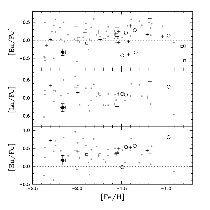
Figure 8: Abundances of the neutron capture elements. Crosses are old halo clusters, open circles are younger halo clusters, open squares are thick disk clusters, and grey dots are field stars (Burris et al. 2000). M68 is represented by filled circles.

Burris et al. (2000) studied abundances of neutron capture elements in a large sample of metal-poor giants, finding that a large star-to-star variations in the neutron capture elemental abundances (see also Gilroy et al. 1988, McWilliam et al. 1995). They suggested that this scatter in neutron capture elemental abundances results from inhomogeneity of the proto-stellar material polluted by SNe II nucleosynthesis ejecta at early stage in the Galaxy’s history. Whether this is the correct interpretation or whether the analyses themselves are partly responsible for the scatter remains to be seen (see Cayrel et al. 2004). In Figure 8, we show Ba, La, and Eu abundances for globular clusters (Brown et al. 1997, 1999; Gratton et al. 1986; Gratton 1987; Gratton & Ortolani 1989; Ivans et al. 1999, 2001; Kraft et al. 1998; Lee & Carney 2002; McWilliam et al. 1992; Shetrone & Keane 2000; Sneden et al. 1997, 2000a, 2000b, 2004) and field stars (Burris et al. 2000) as a function of metallicity. Table 11 summarizes mean Ba, La, Eu abundances for M68 and M15 (Sneden et al. 1997, 2000a), other globular clusters, and field stars with $-$2.50 $\leq$ [Fe/H] $\leq$ $-$1.90 (Burris et al. 2000).

The comparison with M15 and other clusters and stars is not quite so simple, however, as it appears. Sneden et al. (1997) discovered that whereas the abundances of the lighter elements silicon, calcium, and titanium did not vary from star to star, those of the neutron capture elements did, and by factors of four to five. Like the variation in [Si/Ti] seen between M68 and other clusters, the variations in [Ba/Fe] and [Eu/Fe] seen by Sneden et al. (1997, 2000) warn us that we cannot assume all supernovae produce the same heavy element abundance yields. In the case of M15, the lack of variations in the abundances of the light elements would predict in such a simple model that barium and other $s$-process elements and the $r$-process element europium should likewise be constant, contrary to what was seen.

How does M68 fit into this picture? In Figure 9 we reproduce the [Ba/Fe] vs. [Eu/Fe] abundances found by Sneden et al. (1997). The dotted line shows the solar abundances, and the dashed line, displaced from the solar relation by 0.41 dex, shows the mean behavior of the stars in M15, which are plotted as dots. As Sneden et al. (1997) noted, the behavior of the stars in M15 is consistent with an enhanced $r$-process contribution to the abundances of both barium and europium in M15. That process produced different absolute amounts of the neutron capture elements in stars in M15, but the process itself yielded the same relative abundances of the two elements. Our results for the stars in M68 are consistent with this general picture, in that the barium and europium abundance ratio is constant, and essentially the same in M68 and in M15. Sneden et al. (1997) found that the “low barium” and “high barium” groups of stars in M15 had similar [Ba/Eu] ratios, $-0.41\pm 0.03$ ($\sigma=0.13$) dex for all eighteen stars. Our seven stars, including the post-AGB star 117, yield $<$[Ba/Eu]$>$ = $-0.43\pm 0.05$ ($\sigma=0.13$) dex. What is different between the two clusters, however, is that both barium and europium are lower in abundance in M68 than the stars in M15, even the “low barium” stars. Thus M68 was slightly less enriched in $r$-process nucleosynthesis, relative to iron. We could interpret our results in an alternative fashion, that iron is enhanced relative to the $r$-process elements, in this case including barium and europium.

For [La/Eu] we must turn to the smaller sample of Sneden et al. (2000), who studied three stars in M15 with very different [Ba/Fe] ratios, $-0.24$, +0.05, and +0.05. The [La/Fe] values also vary greatly for these three stars: $-0.02$, +0.38, and +0.61, yet the variation seen in [La/Eu] is much smaller, and consistent with the measurement uncertainties: $-0.33$, $-0.45$, and $-0.26$, for a mean value of $-0.35\pm 0.06$ ($\sigma=0.10$) dex. We were able to estimate [La/Eu] values for three of our program stars, and we find $<$[La/Eu]$>$ = $-0.38\pm 0.10$ ($\sigma=0.17$) dex. Thus for both lanthanum and barium, it appears the $r$ process is dominating the nucleosynthesis enrichment in both M68 and in M15, and yielding constant relative abundances of the elements. But as in the case of barium and europium, there is an underabundance of lanthanum relative to iron in M68 compared to M15.

5.4 Summary of Differences Between M68 and M15 and Other Clusters

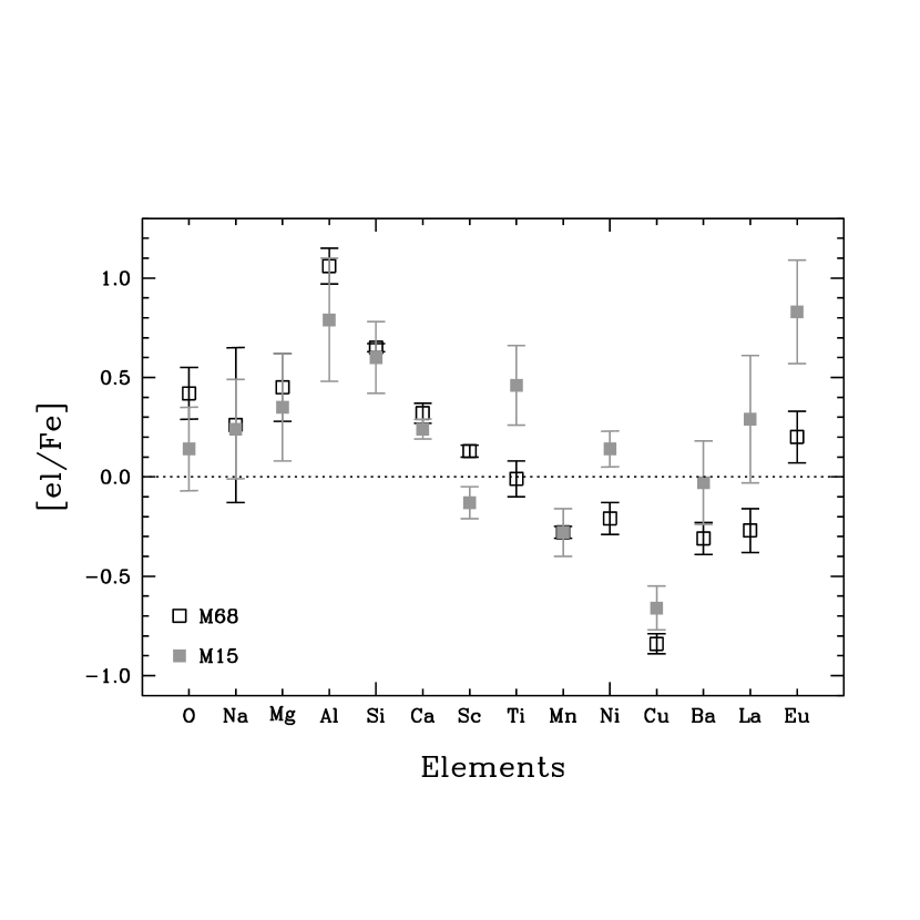
Figure 10: Comparison of elemental abundances between M68 and M15.

In Figure 10, we summarize graphically the many similarities between the abundances of various elements, relative to iron, in M68 compared to M15. Perhaps the two most striking differences are in the much lower titanium abundances in M68, which, as we have seen, might be explained by a greater contribution from more massive stars and their supernovae events in M68 relative to M15. On the other hand, while it appears that the $r$-process has dominated the production of the “traditional” $s$-process elements lanthanum and barium, and that the [La/Eu] and [Ba/Eu] ratios are the same for all the stars in both clusters, the overall $r$-process enrichment varies within M15 (Sneden et al. 1997) and between M68 and M15. The clusters have clearly experienced somewhat different chemical enrichment histories, and it will be interesting to see if models of supernovae enrichment ultimately prove successful in explaining these differences and what this means for the histories and, perhaps, ages of these clusters.

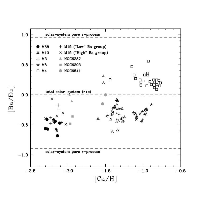
Figure 11: Comparisons of [Ba/Eu] ratios as a function of [Ca/H] of our program stars in M68 and individual stars in other globular clusters.

Finally, in Figure 11 we show the results for individual stars in the abundance ratio of barium and europium, plotted against [Ca/H] rather than [Fe/H]. As Sneden et al. (1997) commented, calcium is thought to be produed in Type II supernovae, compared to iron, whose abundance is more strongly affected by contributions from Type Ia supernovae. Also following Sneden et al. (1997), we show the levels expected from “pure” $r$-process nucleosynthesis, “pure” $s$-process nucleosynthesis, and the intermediate case found to exist in the solar system. At lower [Ca/H] levels, [Ba/Eu] ratios more consistent with $r$-process domination are apparent, which is not terribly surprising. But M68 appears to be one of the most extreme cases.

6 CONCLUSIONS

A chemical abundance study of seven giant stars in M68 has been presented. We estimate the stars’ temperatures using the abundances derived from Fe I lines with differing excitation potentials, but the gravity has been derived using available photometry rather than a comparison between abundances from pressure-insensitive Fe I lines and pressure-sensitive Fe II line. The “spectroscopic” gravities do not agree with the photometric gravities, suggesting non-LTE effects are present. Using only the Fe II lines, which should be less sensitive to non-LTE, and photometric gravities, we find [Fe/H] = $-$2.16 $\pm$ 0.02 ($\sigma=0.04$. We have compared our results to those of Gratton & Ortolani (1989), who found a higher value. We attribute the difference to the lower-resolution spectra available to them at the time. Our results do agree well with those obtained by Minniti et al. (1993), but we regard the agreement as accidental since we could not reproduce their results using their data.

We determine element-to-iron ratios using neutral vs. neutral and ionized vs. ionized lines to again minimize non-LTE effects. We find a large range in sodium abundances, but no significant range in oxygen abundances. Further, the post-AGB star M68-117 does not appear to show any enhancement of sodium. These results are not consistent with deep mixing being the cause of the variations among the light elements oxygen, sodium, magnesium, and aluminum.

There are two notable differences between M68 and the comparably metal-poor cluster M15. While both show enhanced [Si/Fe] ratios relative to other clusters and comparably metal-poor field stars, M68 is quite deficient in titanium compared to M15 or any other cluster. It is possible that this arose because nucleosynthesis enrichment of the stars in M68 was provided by supernovae resulting from the deaths of somewhat more massive progenitors. This would be difficult to reconcile with the nominal younger age for M68 compared to M15, based on the morphologies of their horizontal branch stars’ distribution in temperature/color. Perhaps age is not the only “second parameter”?

The second interesting difference is that [La/Eu] and [Ba/Eu] ratios are similar for the stars in M68 and in M15 (and in both its “high barium” and “low barium” groups of stars—Sneden et al. 1997). This suggests that in both clusters the $r$ process is making a major contribution to the abundance levels of the “traditional” $s$-process elements lanthanum and barium. However, whatever the process is, it is not contributing quite as much to the neutron capture elements’ abundances in M68 as in M15.

Table 1: Journal of observations.

Star			Position (2000)		$V$	$(B-V)$	$K$	$K$	Date/Time	$t_{exp}$	S/N
W	Alt.		$\alpha$	$\delta$						(min)
93	I–82		12:39:20.9	$-$26:46:54	12.67	1.32	9.53	9.57	1996 May 4	120	170
117	ZNG2		12:39:22.5	$-$26:45:12	12.69	1.19	9.73	9.73	1996 May 6	120	115
160	I–260		12:39:24.7	$-$26:43:33	12.69	1.32	9.52	9.53	1996 May 4	120	160
89	A–14		12:39:20.8	$-$26:41:39	12.71	1.33	9.55	9.57	1996 May 4	120	160
412	I–144		12:39:30.8	$-$26:47:53	12.91	1.25	9.88	9.90	1996 May 6	170	140
350			12:39:29.4	$-$26:44:23	13.18	1.15	$\cdots$	10.22	1996 May 5	190	140
48			12:39:15.9	$-$26:45:15	13.35	1.10	$\cdots$	10.53	1996 May 7	130	90

Table 2: Equivalent widths.

$\lambda$ (Å)	Elem.	$\chi$ (eV)	$\log gf$	93	117	160	89	412	350	48	Ref.
6300.23	[O I]	0.000	$-$9.750	29	40	22	43	27	30	$\cdots$	1
6363.88	[O I]	0.020	$-$10.250	$\cdots$	8	8	9	$\cdots$	$\cdots$	$\cdots$	1
5682.63	Na I	2.102	$-$0.700	24	$\cdots$	5	$\cdots$	13	$\cdots$	19	2
5688.22	Na I	2.100	$-$0.460	44	13	9	8	26	31	$\cdots$	2
6160.75	Na I	2.104	$-$1.260	11	$\cdots$	$\cdots$	$\cdots$	6	8	$\cdots$	3
5528.42	Mg I	4.350	$-$0.360	92	110	115	115	105	89	101	4
5711.10	Mg I	4.340	$-$1.630	23	37	42	40	25	$\cdots$	25	4
6696.03	Al I	3.140	$-$1.570	16	$\cdots$	$\cdots$	$\cdots$	8	11	$\cdots$	5
6698.67	Al I	3.140	$-$1.890	7	$\cdots$	$\cdots$	$\cdots$	5	4	$\cdots$	5
5665.56	Si I	4.920	$-$2.040	7	7	7	$\cdots$	7	$\cdots$	$\cdots$	6
5793.08	Si I	4.930	$-$2.060	7	8	$\cdots$	$\cdots$	$\cdots$	6	$\cdots$	6
6243.82	Si I	5.616	$-$1.270	5	$\cdots$	$\cdots$	$\cdots$	6	$\cdots$	$\cdots$	4
6244.48	Si I	5.616	$-$1.270	$\cdots$	$\cdots$	$\cdots$	$\cdots$	5	$\cdots$	$\cdots$	4
5590.11	Ca I	2.521	$-$0.710	32	34	37	$\cdots$	28	27	20	4
5594.46	Ca I	2.523	0.097	78	78	78	$\cdots$	73	61		7
6161.30	Ca I	2.523	$-$1.266	15	15	15	15	12	8	$\cdots$	7
6166.44	Ca I	2.521	$-$1.142	18	15	17	16	14	10	$\cdots$	7
6169.04	Ca I	2.523	$-$0.797	31	27	33	33	29	25	19	7
6169.56	Ca I	2.526	$-$0.478	45	41	49	$\cdots$	40	33	36	7
6455.60	Ca I	2.523	$-$1.290	$\cdots$	12	13	13	$\cdots$	$\cdots$	$\cdots$	7
6471.66	Ca I	2.526	$-$0.686	43	35	37	52	$\cdots$	32	23	7
6499.65	Ca I	2.523	$-$0.818	32	28	34	39	27	24	$\cdots$	7
7148.15	Ca I	2.709	0.137	85	82	86	89	$\cdots$	62	65	7
5526.79	Sc I	1.768	$-$0.256	75	75	79	77	73	62	62	12
5657.90	Sc I	1.507	$-$0.645	69	76	67	71	63	64	62	12
6245.64	Sc I	1.507	$-$1.134	37	35	$\cdots$	41	37	27	23	12
6604.60	Sc I	1.357	$-$1.309	36	33	33	31	29	24	22	12
5866.45	Ti I	1.067	$-$0.784	28	23	37	31	21	16	15	8
5899.30	Ti I	1.053	$-$1.098	15	13	$\cdots$	17	14	$\cdots$	$\cdots$	8
5922.11	Ti I	1.046	$-$1.410	11	11	15	11	$\cdots$	6	$\cdots$	9
5953.16	Ti I	1.887	$-$0.273	10	$\cdots$	15	$\cdots$	$\cdots$	$\cdots$	$\cdots$	10
5965.83	Ti I	1.879	$-$0.353	7	$\cdots$	$\cdots$	10	$\cdots$	$\cdots$	$\cdots$	10
5978.54	Ti I	1.870	$-$0.500	$\cdots$	8	9	$\cdots$	$\cdots$	$\cdots$	$\cdots$	4
6126.22	Ti I	1.067	$-$1.369	$\cdots$	$\cdots$	$\cdots$	10	8	$\cdots$	$\cdots$	9
6258.11	Ti I	1.440	$-$0.299	27	25	34	34	21	16	13	10
6258.71	Ti I	1.460	$-$0.270	35	25	40	36	24	20	15	10
6261.11	Ti I	1.430	$-$0.423	26	20	30	29	19	15	10	10
6606.95	Ti II	2.061	$-$2.790	5	8	8	5	5	4	$\cdots$	11
7214.74	Ti II	2.590	$-$1.740	11	14	13	10	12	10	$\cdots$	11
6021.79	Mn I	3.080	0.030	21	22	22	21	17	16	10	12
5662.51	Fe I	4.178	$-$0.590	26	28	26	30	22	21	15	16
5701.55	Fe I	2.559	$-$2.216	56	52	57	55	49	41	39	14
5753.12	Fe I	4.260	$-$0.705	17	$\cdots$	17	17	16	14	13	16
5816.37	Fe I	4.549	$-$0.618	10	$\cdots$	$\cdots$	10	$\cdots$	$\cdots$	$\cdots$	16
5916.25	Fe I	2.453	$-$2.994	24	21	28	24	23	$\cdots$	10	13
5956.69	Fe I	0.859	$-$4.608	64	58	$\cdots$	69	50	$\cdots$	$\cdots$	15
6027.05	Fe I	4.076	$-$1.106	13	$\cdots$	13	14	11	11	$\cdots$	16
6065.48	Fe I	2.609	$-$1.530	97	88	102	96	85	75	77	14
6082.71	Fe I	2.223	$-$3.573	$\cdots$	13	17	17	13	$\cdots$	$\cdots$	13
6151.62	Fe I	2.176	$-$3.299	28	26	33	31	23	21	17	13
6173.34	Fe I	2.223	$-$2.880	48	$\cdots$	53	44	40	35	32	13
6180.20	Fe I	2.728	$-$2.637	23	$\cdots$	$\cdots$	21	$\cdots$	$\cdots$	11	18
6200.31	Fe I	2.609	$-$2.437	42	40	45	42	37	30	28	14
6219.28	Fe I	2.198	$-$2.433	84	74	84	82	67	65	50	13
6229.23	Fe I	2.845	$-$2.846	$\cdots$	$\cdots$	13	12	$\cdots$	10	$\cdots$	17
6230.73	Fe I	2.559	$-$1.281	126	114	120	122	111	102	95	14
6232.64	Fe I	3.654	$-$1.283	27	28	29	28	23	$\cdots$	17	18
6246.32	Fe I	3.603	$-$0.894	52	53	58	54	52	41	35	16
6252.55	Fe I	2.404	$-$1.687	108	100	112	109	102	90	83	13
6265.13	Fe I	2.176	$-$2.550	79	68	83	81	66	64	54	13
6270.22	Fe I	2.858	$-$2.505	$\cdots$	19	$\cdots$	20	16	$\cdots$	$\cdots$	17
6322.69	Fe I	2.588	$-$2.426	41	45	51	45	41	36	28	14
6335.33	Fe I	2.198	$-$2.194	91	87	$\cdots$	99	81	77	67	16
6336.82	Fe I	3.686	$-$0.916	$\cdots$	41	$\cdots$	$\cdots$	$\cdots$	$\cdots$	$\cdots$	18
6344.15	Fe I	2.433	$-$2.923	33	27	36	36	28	24	18	13
6393.60	Fe I	2.433	$-$1.469	117	108	118	116	105	99	92	17
6408.02	Fe I	3.686	$-$1.066	35	34	40	41	29	31	23	17
6411.65	Fe I	3.654	$-$0.734	59	59	65	61	54	43	42	16
6421.35	Fe I	2.280	$-$2.027	104	100	110	106	94	81	79	13
6430.84	Fe I	2.176	$-$2.006	107	108	115	114	109	92	78	13
6481.87	Fe I	2.279	$-$2.984	47	42	52	$\cdots$	41	$\cdots$	$\cdots$	13
6494.98	Fe I	2.404	$-$1.273	142	136	131	140	128	$\cdots$	107	13
6498.94	Fe I	0.958	$-$4.687	52	42	62	49	37	36	26	15
6574.23	Fe I	0.990	$-$5.004	25	26	36	34	26	17	13	15
6575.02	Fe I	2.588	$-$2.727	27	29	33	32	27	23	13	16
6581.21	Fe I	1.485	$-$4.707	13	$\cdots$	17	14	$\cdots$	$\cdots$	$\cdots$	17
6592.91	Fe I	2.728	$-$1.490	98	88	96	94	87	79	68	16
6593.87	Fe I	2.433	$-$2.422	67	55	65	69	56	50	38	13
6609.11	Fe I	2.559	$-$2.692	32	35	38	36	33	24	16	14
6625.02	Fe I	1.011	$-$5.366	13	$\cdots$	19	14	12	9	$\cdots$	15
6663.44	Fe I	2.420	$-$2.479	62	62	70	64	54	47	41	13
6677.99	Fe I	2.692	$-$1.435	105	104	109	103	98	89	77	16
6750.15	Fe I	2.424	$-$2.621	51	50	62	60	50	42	34	13
6978.85	Fe I	2.484	$-$2.500	57	48	67	58	51	41	35	13
7223.66	Fe I	3.017	$-$2.269	25	25	28	27	24	18	$\cdots$	18
7511.01	Fe I	4.178	0.082	75	70	74	74	64	59	50	16
7710.36	Fe I	4.220	$-$1.129	$\cdots$	$\cdots$	13	$\cdots$	$\cdots$	$\cdots$	$\cdots$	16
7723.20	Fe I	2.279	$-$3.617	18	$\cdots$	20	14	13	$\cdots$	$\cdots$	13
5991.38	Fe II	3.153	$-$3.557	$\cdots$	12	$\cdots$	$\cdots$	$\cdots$	$\cdots$	$\cdots$	19
6149.26	Fe II	3.889	$-$2.724	10	12	$\cdots$	10	$\cdots$	$\cdots$	$\cdots$	19
6247.56	Fe II	3.891	$-$2.329	$\cdots$	$\cdots$	21	25	19	20	19	19
6416.92	Fe II	3.891	$-$2.740	$\cdots$	12	$\cdots$	$\cdots$	$\cdots$	$\cdots$	$\cdots$	19
6432.68	Fe II	2.891	$-$3.708	20	22	19	21	19	18	15	19
6456.38	Fe II	3.903	$-$2.075	33	32	29	31	32	31	24	19
6176.81	Ni I	4.088	$-$0.530	6	$\cdots$	$\cdots$	$\cdots$	$\cdots$	$\cdots$	$\cdots$	20
6586.31	Ni I	1.951	$-$2.810	15	10	22	18	14	8	$\cdots$	20
6643.63	Ni I	1.676	$-$2.010	80	67	87	80	70	55	55	4
6767.77	Ni I	1.826	$-$2.170	71	57	74	66	58	44	34	20
5782.13	Cu I	1.642	$-$1.700	11	$\cdots$	11	9	$\cdots$	6	$\cdots$	21
5853.69	Ba II	0.600	$-$1.010	72	56	69	74	65	62	63	5
6141.73	Ba II	0.700	$-$0.080	131	109	120	113	117	113	103	5
6496.91	Ba II	0.600	$-$0.380	127	109	119	122	119	113	98	5
6390.48	La II	0.321	$-$1.410	5	$\cdots$	5	$\cdots$	6	$\cdots$	$\cdots$	4
6774.27	La II	0.126	$-$1.750	7	$\cdots$	$\cdots$	$\cdots$	6	$\cdots$	$\cdots$	4
6645.06	Eu II	1.380	0.204	6	5	8	9	7	10	$\cdots$	22
7217.55	Eu II	1.230	$-$0.301	3	$\cdots$	7	8	$\cdots$	$\cdots$	$\cdots$	22
7426.57	Eu II	1.279	$-$0.149	5	$\cdots$	$\cdots$	$\cdots$	$\cdots$	$\cdots$	$\cdots$	22

Table 3: References for $\log gf$ values.

Ref. No.	Reference	Elem.
1	Lambert (1978)	[O I]
2	Ivans et al. (2001)	Na I
3	Kraft et al. (1992)	Na I
4	Sneden et al. (2004)	Mg I, Si I, Ca I,
		Ti I, Ni I, La II
5	Sneden et al. (1997)	Al I, Ba II
6	Garz (1973)	Si I
7	Smith (1981)	Ca I
8	Blackwell et al. (1982a)	Ti I
9	Blackwell et al. (1983)	Ti I
10	Blackwell et al. (1986b)	Ti I
11	Fuhr et al. (1988a)	Ti II
12	Prochaska & McWilliam (2000)	Sc I, Mn I
13	Blackwell et al. (1982b)	Fe I
14	Blackwell et al. (1982c)	Fe I
15	Blackwell et al. (1986a)	Fe I
16	O’Brian et al. (1991)	Fe I
17	Bard et al. (1991)	Fe I
18	Bard & Kock (1994)	Fe I
19	Biémont (1991)	Fe II
20	Fuhr et al. (1988b)	Ni I
21	Kurucz  (1993)	Cu I
22	Biémont et al. (1982)	Eu II

Table 4: Model atmosphere parameters.

Star		$T_{\rm eff}$(K)						$\log g$	$\log g$	$v_{\rm turb}$
		$(B-V)$	$(V-K)$		(FPC83)	(spec)		(phot)	(spec)	(km s-1)
			(FPC83)	(2MASS)
93		4220	4215	4240	4287	4200		0.7	0.1	1.95
117		4370	4340	4335	4501	4300		0.8	0.3	1.80
160		4200	4200	4200	4329	4100		0.7	0.0	1.80
89		4200	4200	4215	4279	4175		0.7	0.0	1.90
412		4275	4290	4300	4372	4200		0.8	0.1	1.75
350		4390	$\cdots$	4340	$\cdots$	4300		1.0	0.3	1.60
48		4450	$\cdots$	4450	$\cdots$	4325		1.1	0.3	1.75

Table 5: Elemental abundances of M68 with photometric $\log g$.

	93	117	160	89	412	350	48	Mean	Mean
[Fe/H]I	$-$2.50	$-$2.38	$-$2.56	$-$2.51	$-$2.58	$-$2.53	$-$2.67	$-$2.53	$-$2.56
n	43	38	42	45	42	35	35	7	6
$\sigma$	0.05	0.06	0.05	0.05	0.06	0.05	0.06	0.09	0.06
[Fe/H]II	$-$2.17	$-$2.16	$-$2.12	$-$2.14	$-$2.16	$-$2.15	$-$2.23	$-$2.16	$-$2.16
n	3	5	3	4	3	3	3	7	6
$\sigma$	0.03	0.05	0.02	0.06	0.05	0.02	0.06	0.03	0.04
[O/Fe]	+0.37	+0.46	+0.23	+0.43	+0.37	+0.51	+0.59	+0.42	+0.42
n	1	2	2	2	1	1	2	7	6
$\sigma$	$\cdots$	0.20	0.01	0.20	$\cdots$	$\cdots$	0.05	0.12	0.13
[Na/Fe]	+0.62	$-$0.07	$-$0.23	$-$0.27	+0.38	+0.55	+0.39	+0.23	+0.24
n	3	1	2	1	3	2	1	7	6
$\sigma$	0.07	$\cdots$	0.00	$\cdots$	0.08	0.05	$\cdots$	0.40	0.39
[Mg/Fe]	+0.12	+0.39	+0.50	+0.47	+0.35	+0.19	+0.45	+0.35	+0.35
n	2	2	2	2	2	1	2	7	6
$\sigma$	0.05	0.01	0.01	0.01	0.10	$\cdots$	0.03	0.14	0.16
[Al/Fe]	+1.18	$\cdots$	$\cdots$	$\cdots$	+1.00	+1.07	$\cdots$	+1.08	+1.08
n	2	$\cdots$	$\cdots$	$\cdots$	2	2	$\cdots$	3	3
$\sigma$	0.05	$\cdots$	$\cdots$	$\cdots$	0.07	0.07	$\cdots$	0.09	0.09
[Si/Fe]	+0.68	+0.65	+0.77	$\cdots$	+0.75	+0.72	$\cdots$	+0.71	+0.73
n	3	2	1	$\cdots$	3	1	$\cdots$	5	4
$\sigma$	0.05	0.04	$\cdots$	$\cdots$	0.05	$\cdots$	$\cdots$	0.05	0.04
[Ca/Fe]	+0.33	+0.27	+0.29	+0.37	+0.30	+0.23	+0.32	+0.30	+0.31
n	9	10	10	7	7	9	5	7	6
$\sigma$	0.05	0.07	0.04	0.08	0.04	0.07	0.05	0.04	0.05
[Sc/Fe]II	+0.14	+0.19	+0.16	+0.14	+0.13	+0.07	+0.13	+0.14	+0.13
n	4	4	3	4	4	4	4	7	6
$\sigma$	0.14	0.20	0.25	0.20	0.18	0.18	0.18	0.04	0.03
[Ti/Fe]I	+0.06	+0.07	+0.09	+0.03	$-$0.02	$-$0.02	+0.01	+0.03	+0.02
n	8	6	7	8	6	5	4	7	6
$\sigma$	0.07	0.05	0.07	0.05	0.04	0.06	0.05	0.04	0.05
[Ti/Fe]II	$-$0.12	+0.09	+0.01	$-$0.15	$-$0.06	$-$0.08	$\cdots$	$-$0.05	$-$0.08
n	2	2	2	2	2	2	$\cdots$	6	5
$\sigma$	0.03	0.12	0.08	0.05	0.01	0.02	$\cdots$	0.09	0.06
[Ti/Fe]mean	$-$0.03	+0.08	+0.05	$-$0.06	$-$0.04	$-$0.05	+0.01	$-$0.01	$-$0.03
[Mn/Fe]	$-$0.25	$-$0.22	$-$0.30	$-$0.27	$-$0.29	$-$0.26	$-$0.33	$-$0.27	$-$0.28
n	1	1	1	1	1	1	1	7	6
$\sigma$	$\cdots$	$\cdots$	$\cdots$	$\cdots$	$\cdots$	$\cdots$	$\cdots$	0.04	0.03
[Ni/Fe]	$-$0.04	$-$0.21	$-$0.01	$-$0.09	$-$0.09	$-$0.22	$-$0.14	$-$0.11	$-$0.10
n	4	3	3	3	3	3	2	7	6
$\sigma$	0.11	0.11	0.08	0.09	0.09	0.09	0.00	0.08	0.07
[Cu/Fe]	$-$0.74	$\cdots$	$-$0.83	$-$0.86	$\cdots$	$-$0.85	$\cdots$	$-$0.82	$-$0.82
n	1	$\cdots$	1	1	$\cdots$	1	$\cdots$	4	4
$\sigma$	$\cdots$	$\cdots$	$\cdots$	$\cdots$	$\cdots$	$\cdots$	$\cdots$	0.05	0.05
[Ba/Fe]II	$-$0.28	$-$0.46	$-$0.39	$-$0.40	$-$0.30	$-$0.19	$-$0.32	$-$0.33	$-$0.31
n	3	3	3	3	3	3	3	7	6
$\sigma$	0.09	0.12	0.06	0.10	0.12	0.14	0.04	0.09	0.08
[La/Fe]II	$-$0.23	$\cdots$	$-$0.40	$\cdots$	$-$0.19	$\cdots$	$\cdots$	$-$0.27	$-$0.27
n	2	$\cdots$	1	$\cdots$	2	$\cdots$	$\cdots$	3	3
$\sigma$	0.14	$\cdots$	$\cdots$	$\cdots$	0.03	$\cdots$	$\cdots$	0.11	0.11
[Eu/Fe]II	+0.06	+0.01	+0.18	+0.28	+0.11	+0.37	$\cdots$	+0.17	+0.20
n	3	1	2	2	1	1	$\cdots$	6	5
$\sigma$	0.08	$\cdots$	0.13	0.12	$\cdots$	$\cdots$	$\cdots$	0.14	0.13

Table 6: Elemental abundances of M68 spectroscopic $\log g$.

	93	117	160	89	412	350	48	Mean	Mean
[Fe/H]I	$-$2.40	$-$2.30	$-$2.46	$-$2.40	$-$2.47	$-$2.43	$-$2.56	$-$2.43	$-$2.45
n	43	38	42	45	42	35	35	7	6
$\sigma$	0.05	0.06	0.05	0.06	0.06	0.05	0.07	0.08	0.06
[Fe/H]II	$-$2.37	$-$2.33	$-$2.35	$-$2.36	$-$2.39	$-$2.39	$-$2.52	$-$2.39	$-$2.40
n	3	5	3	4	3	3	3	7	6
$\sigma$	0.02	0.05	0.02	0.06	0.04	0.02	0.06	0.06	0.06
[Fe/H]mean	$-$2.39	$-$2.32	$-$2.41	$-$2.38	$-$2.43	$-$2.41	$-$2.54	$-$2.43	$-$2.41
[O/Fe]	+0.38	+0.43	+0.23	+0.42	+0.39	+0.51	+0.60	+0.42	+0.42
n	1	2	2	2	1	1	2	7	6
$\sigma$	$\cdots$	0.20	0.01	0.21	$\cdots$	$\cdots$	0.06	0.11	0.13
[Na/Fe]	+0.65	$-$0.04	$-$0.21	$-$0.24	+0.38	+0.56	+0.40	+0.21	+0.26
n	3	1	2	1	3	2	1	7	6
$\sigma$	0.08	$\cdots$	0.00	$\cdots$	0.07	0.05	$\cdots$	0.37	0.39
[Mg/Fe]	+0.19	+0.48	+0.60	+0.60	+0.43	+0.32	+0.53	+0.45	+0.45
n	2	2	2	2	2	1	2	7	6
$\sigma$	0.03	0.06	0.08	0.08	0.21	$\cdots$	0.13	0.15	0.17
[Al/Fe]	+1.16	$\cdots$	$\cdots$	$\cdots$	+0.98	+1.04	$\cdots$	+1.06	+1.06
n	2	$\cdots$	$\cdots$	$\cdots$	2	2	$\cdots$	3	3
$\sigma$	0.06	$\cdots$	$\cdots$	$\cdots$	0.07	0.07	$\cdots$	0.09	0.09
[Si/Fe]	+0.62	+0.63	+0.67	$\cdots$	+0.66	+0.64	$\cdots$	+0.64	+0.65
n	3	2	1	$\cdots$	3	1	$\cdots$	5	4
$\sigma$	0.06	0.04	$\cdots$	$\cdots$	0.06	$\cdots$	$\cdots$	0.02	0.02
[Ca/Fe]	+0.36	+0.31	+0.31	+0.39	+0.31	+0.24	+0.32	+0.32	+0.32
n	9	10	10	7	7	9	5	7	6
$\sigma$	0.04	0.08	0.07	0.09	0.06	0.07	0.05	0.05	0.05
[Sc/Fe]II	+0.23	+0.22	+0.33	+0.23	+0.24	+0.14	+0.20	+0.23	+0.23
n	4	4	3	4	4	4	4	7	6
$\sigma$	0.19	0.22	0.34	0.26	0.24	0.22	0.22	0.06	0.06
[Ti/Fe]I	+0.06	+0.08	+0.06	+0.08	$-$0.04	$-$0.02	+0.01	+0.03	+0.03
n	8	6	7	8	6	5	4	7	6
$\sigma$	0.07	0.05	0.09	0.06	0.04	0.06	0.06	0.05	0.05
[Ti/Fe]II	$-$0.10	+0.08	+0.06	$-$0.15	$-$0.02	$-$0.06	$\cdots$	$-$0.03	$-$0.05
n	2	2	2	2	2	2	$\cdots$	6	5
$\sigma$	0.02	0.13	0.10	0.06	0.00	0.03	$\cdots$	0.09	0.08
[Ti/Fe]mean	$-$0.02	+0.08	+0.06	$-$0.04	$-$0.03	$-$0.04	+0.01	+0.00	$-$0.01
[Mn/Fe]	$-$0.24	$-$0.19	$-$0.31	$-$0.25	$-$0.30	$-$0.26	$-$0.33	$-$0.27	$-$0.28
n	1	1	1	1	1	1	1	7	6
$\sigma$	$\cdots$	$\cdots$	$\cdots$	$\cdots$	$\cdots$	$\cdots$	$\cdots$	0.05	0.04
[Ni/Fe]	$-$0.04	$-$0.22	$-$0.13	$-$0.16	$-$0.18	$-$0.27	$-$0.19	$-$0.17	$-$0.16
n	4	3	3	3	3	3	2	7	6
$\sigma$	0.11	0.11	0.09	0.09	0.09	0.09	0.00	0.07	0.08
[Cu/Fe]	$-$0.76	$\cdots$	$-$0.90	$-$0.88	$\cdots$	$-$0.87	$\cdots$	$-$0.86	$-$0.86
n	1	$\cdots$	1	1	$\cdots$	1	$\cdots$	4	4
$\sigma$	$\cdots$	$\cdots$	$\cdots$	$\cdots$	$\cdots$	$\cdots$	$\cdots$	0.06	0.06
[Ba/Fe]II	$-$0.18	$-$0.44	$-$0.24	$-$0.31	$-$0.18	$-$0.12	$-$0.24	$-$0.24	$-$0.21
n	3	3	3	3	3	3	3	7	6
$\sigma$	0.11	0.11	0.05	0.10	0.12	0.13	0.06	0.11	0.07
[La/Fe]II	$-$0.20	$\cdots$	$-$0.33	$\cdots$	$-$0.15	$\cdots$	$\cdots$	$-$0.23	$-$0.23
n	2	$\cdots$	1	$\cdots$	2	$\cdots$	$\cdots$	3	3
$\sigma$	0.13	$\cdots$	$\cdots$	$\cdots$	0.02	$\cdots$	$\cdots$	0.10	0.10
[Eu/Fe]II	+0.06	+0.01	+0.24	+0.28	+0.15	+0.39	$\cdots$	+0.18	+0.22
n	3	1	2	2	1	1	$\cdots$	6	5
$\sigma$	0.08	$\cdots$	0.12	0.11	$\cdots$	$\cdots$	$\cdots$	0.14	0.13

Table 7: Differences in elemental abundances using photometric and spectroscopic surface gravities.

Elem.	[el/Fe]phot $-$ [el/Fe]spec
[Fe/H]	+0.25 $\pm$ 0.05
[O/Fe]	+0.01 $\pm$ 0.01
[Na/Fe]	$-$0.02 $\pm$ 0.01
[Mg/Fe]	$-$0.10 $\pm$ 0.02
[Al/Fe]	+0.02 $\pm$ 0.01
[Si/Fe]	+0.07 $\pm$ 0.03
[Ca/Fe]	$-$0.02 $\pm$ 0.01
[Sc/Fe]II	$-$0.09 $\pm$ 0.04
[Ti/Fe]I	+0.00 $\pm$ 0.03
[Ti/Fe]II	$-$0.02 $\pm$ 0.02
[Ti/Fe]mean	$-$0.01 $\pm$ 0.01
[Mn/Fe]	$-$0.01 $\pm$ 0.02
[Ni/Fe]	+0.05 $\pm$ 0.04
[Cu/Fe]	+0.03 $\pm$ 0.03
[Ba/Fe]II	$-$0.10 $\pm$ 0.04
[La/Fe]II	$-$0.05 $\pm$ 0.02
[Eu/Fe]II	$-$0.02 $\pm$ 0.03

Table 8: Abundance dependencies on model atmosphere.

Elem.	$\delta T_{\rm eff}$	$\delta\log g$	$\delta v_{\rm turb}$
	$\pm$ 80	$\pm$ 0.3	$\pm$ 0.2
	(K)		(km s-1)
[Fe/H]I	$\pm$ 0.12	$\mp$ 0.03	$\mp$ 0.03
[Fe/H]II	$\mp$ 0.06	$\pm$ 0.10	$\pm$ 0.02
[O/Fe]	$\pm$ 0.04	$\pm$ 0.05	$\mp$ 0.03
[Na/Fe]	$\pm$ 0.03	$\mp$ 0.03	$\pm$ 0.03
[Mg/Fe]	$\mp$ 0.05	$\mp$ 0.05	$\pm$ 0.01
[Al/Fe]	$\mp$ 0.06	$\mp$ 0.01	$\pm$ 0.03
[Si/Fe]	$\mp$ 0.10	$\pm$ 0.01	$\pm$ 0.04
[Ca/Fe]	$\mp$ 0.04	$\mp$ 0.04	$\pm$ 0.01
[Sc/Fe]II	$\pm$ 0.06	$\mp$ 0.02	$\mp$ 0.01
[Ti/Fe]I	$\pm$ 0.03	$\mp$ 0.02	$\pm$ 0.03
[Ti/Fe]II	$\pm$ 0.04	$\pm$ 0.00	$\pm$ 0.02
[Mn/Fe]	$\mp$ 0.02	$\mp$ 0.03	$\pm$ 0.04
[Ni/Fe]	$\mp$ 0.02	$\pm$ 0.01	$\pm$ 0.01
[Cu/Fe]	$\pm$ 0.01	$\pm$ 0.01	$\pm$ 0.02
[Ba/Fe]II	$\pm$ 0.08	$\mp$ 0.02	$\mp$ 0.09
[La/Fe]II	$\pm$ 0.09	$\mp$ 0.01	$\pm$ 0.02
[Eu/Fe]II	$\pm$ 0.06	$\pm$ 0.00	$\pm$ 0.02

Table 9: Stellar parameters and elemental abundances of the star 160.

	This study	Gratton & Ortolani	Minniti et al.
		(1989)	(1993 & 1996)
$T_{\rm eff}$	4100	4329	4400
(K)
$\log g$	0.7	0.75	1.0
method	phot.	phot.	spec.
$v_{\rm turb}$	1.8	1.6	2.0
(km sec-1)
[Fe/H]I	$-$2.56	$-$1.94	$-$2.11
[Fe/H]II	$-$2.17	$\cdots$	$-$2.14
[O/Fe]	+0.23	+0.22	+0.25
[Na/Fe]	$-$0.23	$-$0.04	$-$0.08
[Mg/Fe]	+0.50	+0.07	$\cdots$
[Si/Fe]	+0.77	+0.41	$\cdots$
[Ca/Fe]	+0.29	+0.25	$\cdots$
[Ti/Fe]	+0.05	+0.43	$\cdots$
[Ni/Fe]	$-$0.01	$-$0.15	$\cdots$
[Ba/Fe]	$-$0.39	$-$0.33	$\cdots$

Table 10: Comparisons of $\alpha$-element abundances.

	[Si/Fe]	[Ca/Fe]	[Ti/Fe]	[$\alpha$/Fe]	n
M68	0.73 $\pm$ 0.02	0.31 $\pm$ 0.02	$-$0.03 $\pm$ 0.04	0.34 $\pm$ 0.22	5,7,7
M15	0.62 $\pm$ 0.06	0.24 $\pm$ 0.01	0.27 $\pm$ 0.08	0.38 $\pm$ 0.12	11,18,4
old halo	0.38 $\pm$ 0.05	0.30 $\pm$ 0.03	0.33 $\pm$ 0.03	0.34 $\pm$ 0.02	15
old inner halo	0.56 $\pm$ 0.05	0.26 $\pm$ 0.07	0.15 $\pm$ 0.06	0.32 $\pm$ 0.03	3
younger halo	0.29 $\pm$ 0.09	0.14 $\pm$ 0.06	0.17 $\pm$ 0.07	0.20 $\pm$ 0.05	7
younger halo	0.38 $\pm$ 0.09	0.21 $\pm$ 0.04	0.25 $\pm$ 0.06	0.28 $\pm$ 0.02	5
disk	0.39 $\pm$ 0.08	0.16 $\pm$ 0.07	0.31 $\pm$ 0.08	0.29 $\pm$ 0.04	4
Field	0.52 $\pm$ 0.04	0.35 $\pm$ 0.03	0.30 $\pm$ 0.04	0.39 $\pm$ 0.02	9, 20, 20

Table 11: Comparisons of neutron capture element abundances.

	[Ba/Fe]	n	[La/Fe]	n	[Eu/Fe]	n
M68	$-$0.31 $\pm$ 0.08		$-$0.27 $\pm$ 0.11		+0.20 $\pm$ 0.13	7,3,6
M15-all	+0.10 $\pm$ 0.21		$\cdots$		+0.49 $\pm$ 0.20	18,0,18
M15-high Ba	+0.23 $\pm$ 0.09		$\cdots$		+0.66 $\pm$ 0.08	10,0,10
M15-low Ba	$-$0.11 $\pm$ 0.06		$\cdots$		+0.29 $\pm$ 0.09	8,0,8
old halo	+0.11 $\pm$ 0.23	16	+0.22 $\pm$ 0.18	5	+0.45 $\pm$ 0.13	8
old inner halo	+0.21 $\pm$ 0.20	3	+0.18 $\pm$ 0.08	3	+0.39 $\pm$ 0.07	3
younger halo	$-$0.03 $\pm$ 0.33	5	+0.17 $\pm$ 0.12	3	+0.48 $\pm$ 0.35	4
younger halo	+0.05 $\pm$ 0.34	3	+0.09	1	+0.56 $\pm$ 0.02	2
disk	$-$0.25 $\pm$ 0.22	4	$\cdots$	$\cdots$	+0.33	1
Field	+0.18 $\pm$ 0.11	27	+0.11 $\pm$ 0.08	14	+0.39 $\pm$ 0.09	17

Figure 1: HB type versus [Fe/H] (HB isochrones) of “halo” globular clusters (Da Costa & Armandroff 1995) and M68. Crosses are “old halo” clusters and open circles are “younger halo” clusters, where large crosses and open circles denote clusters studied employing high-resolution spectroscopy (see also Figure 2). HB isochrones for $\Delta t$ = 0.0, $-$1.1, and $-$2.2 Gyr (with respect to the mean age of “old halo” globular clusters) are also shown with dashed lines (Rey et al. 2001).

Figure 2: Color-magnitude diagram of M68 with photometry from Walker (1994), showing the positions of our program stars.

Figure 3: A comparison of equivalent widths of the star 160 with those of Gratton & Ortolani (1989) and Minniti et al (1993).

Figure 4: Elemental abundances studied in this work plotted against $T_{\rm eff}$. Note that the ordinate of the top panel is [Fe/H], while the ordinates of the remaining panels are [el/Fe] ratios. Neutral atoms are presented by filled circles and singly ionized atoms by open circles. Dashed lines are the mean abundances of each element. The mean Fe II and Ti II abundances are presented by dotted lines.

Figure 5: (a) The $\log$ n(Fe) versus excitation potential relation of the star M68-160 (I260) using Fe I equivalent widths of Minniti et al. (1993) with $\log$(W_λ/$\lambda$) $\leq$ $-5.2$ for $T_{\rm eff}$ = 4400 K, $\log g$ = 1.0, and $v_{\rm turb}$ = 2.0 km s^-1. Crosses are for Fe I lines with W_λ $>$ 10 mÅ and open squares are for W_λ $\leq$ 10 mÅ from Minniti et al. (1993). The dotted and the dashed lines represent the least square fits to the data with and without the Fe I $\lambda$ 6538.84 Å, respectively. Filled circles show the relation using Fe I equivalent widths of this study and the solid line is for the least square fit to the data. (b) Same as (a), but using the model atmosphere with $T_{\rm eff}$ = 4275 K, $\log g$ = 1.0, and $v_{\rm turb}$ = 2.0 km s^-1 and the Fe I $\lambda$ 6538.84 Å line is not used. (c) Same as (b), but using the model atmosphere with $T_{\rm eff}$ = 4100 K, $\log g$ = 0.7, and $v_{\rm turb}$ = 1.8 km s^-1.

Figure 6: A comparison of [Na/Fe] vs. [O/Fe] for M15 (dots) vs. those of M68 (circles). The post-AGB star M68-117 is marked with an open square.

Figure 9: The abundances of barium and europium relative to iron in M15 (dots) and M68 (circles). The post-AGB star M68-117 is marked by an open square. The dotted line represents the solar abundance pattern. The dashed line is the approximate mean for the stars in M15. Despite varying levels of neutron capture abundances in the cluster, the [Ba/Eu] ratio appears to be constant. That is true as well for M68.