2-D Models of Protostars: III. Effects of Stellar Temperature

Abstract

We model how the mid-infrared colors of Young Stellar Objects (YSOs) vary with stellar temperature. The spectral energy distribution (SED) of each object has contributions from thermal emission of circumstellar dust, from direct stellar photospheric emission, and from scattered stellar emission. We first isolate the effects of stellar contributions (direct+scattered) to the SED using homologous “Class I” models: the distribution of circumstellar matter is chosen to scale with stellar temperature $T_{\star}$ such that the shape of the thermal contribution to the SED remains constant. The relative contribution of stellar direct and scattered light varies with $T_{\star}$, changing the $1-10\mu$m (mid-infrared; MIR) colors. Stellar light contributes more to the MIR emission of YSOs with lower temperature stars ($T_{\star}\sim$ 4000 K) because the emission peak wavelength of the star is closer to that of the thermal radiation. In YSOs with hotter central stars, since the peak of the stellar and thermal spectra are more separated in wavelength, the $1-10\mu$m spectrum is closer to a pure thermal spectrum and the objects are redder.

Next we consider realistic Class 0, I, and II source models and find that the other dominant effect of varying stellar temperature on YSO SEDs is that of the inner disk wall: In high-$T_{\star}$ models, the dust destruction radius is much further out with a consequently larger inner disk wall that contributes relatively more to the $2-10\mu$m flux. This effect partially offsets that of the stellar contribution leading to varying behaviors of the $2-10\mu$m flux: In Class 0 sources, the trend is for higher $T_{\star}$ models to have redder colors. In Class I sources, the trend applies with some exceptions. In Class II sources, $2-10\mu$m colors become redder going from $T_{\star}=4000$ to 8000 due to decreasing stellar contribution at $T_{\star}=8000K$, and then become blue again from 8000 to 31500 K due to increasing inner disk wall contribution. Near edge-on inclinations, the color behavior is completely different.

Our modeled MIR protostellar colors have implications for interpretations of Spitzer IRAC observations of star formation regions: It is commonly assumed that the slope of the SED at $1-10\mu$m is directly related to evolutionary state. We show that inclination effects, aperture size, scattered light, and stellar temperature cause a broad spread in the colors of a source at a single evolutionary state. Color-magnitude diagrams can help sort out these effects by separating sources with different $T_{\star}$ based on their different brightness (for sources at the same distance).

1 Introduction

With the launch and successful operation of the Spitzer Space Telescope (Werner et al., 2004), there is a wealth of mid-infrared data being collected on star formation regions near and far (e.g. Allen et al., 2004; Megeath et al., 2004; Reach et al., 2004; Whitney et al., 2004). The IRAC camera (Fazio et al., 2004) provides unprecedented sensitivity and mapping speed using four filters centered on 3.6, 4.5, 5.8, and 8 $\mu$m, and the MIPS camera (Rieke et al., 2004) is functioning particularly well in the 24$\mu$m band (e.g. Muzerolle et al., 2004). Furthermore, many current ground-based facilities and recent space based facilities (e.g. ISO) are optimized to collect data in the near/mid-IR. Thus, in many cases, scientific analysis of star forming clusters is based only on broad-band colors in the 1-30$\mu$m range.

Traditionally the slope of the SED in this region, parameterized by the spectral index $\alpha$ ($=d\log\lambda F_{\lambda}/d\log\lambda$) is used to classify evolutionary state (Lada, 1987, 1999). A sequence of evolutionary classes is fairly well-defined for protostars of moderate mass ($M<1-2M_{\sun}$). Sources for which $\alpha$ is positive are thought to have large (thousands of AU) infalling envelopes and are classified as Class 0 to Class I. Class 0 sources are very young ($10^{4}$ yrs) protostars (André et al. 1993) with high infall rates and very collimated outflows. Class I sources are older ($10^{5}$ yrs) with lower infall rates and larger bipolar cavities carved by meandering jets and molecular outflows (Gómez et al. 1997; Richer et al. 2000; Reipurth et al. 2000). Sources with $\alpha<0$ are identified as Class II sources, pre-main sequence stars surrounded by flared accretion disks. Obviously there are intermediate stages of evolution between Class I and II and it is commonly thought that the spectral index continuum is also a measure of the evolutionary continuum between Class 0 and II (Kenyon & Hartmann, 1995).

Contrasting with the well-defined class system for low-mass stars, the evolution of high-mass protostars is poorly understood. Disk accretion is more difficult to model theoretically in the case of a high-mass protostar because of strong radiation pressure from the central source, high accretion rates, and large disk masses leading to instabilities. Some theorists have suggested protostellar coalescence as an alternative formation mechanism (Bonnell, Bate, & Zinnecker, 1998), but others have succeeded in producing viable accretion models (Behrend & Maeder, 2001; Maeder & Behrend, 2002). The large volume of mid-infrared data currently being collected in protostars of all masses makes it important to understand the infrared properties of high-mass protostars. In particular, does the slope of the SED relate to evolutionary state, as for low-mass stars, and what other effects are present that should be taken into account when analyzing the data?

This paper is part of a series on using 2-D radiative transfer models to interpret data of Young Stellar Objects (YSOs). In previous papers (Whitney et al. 2003a,b; Papers I & II), we showed that inclination effects can blur the separation of evolutionary states in mid-IR color-color diagrams of low-mass YSOs. As an example, in edge-on Class I sources, the mid-IR flux is dominated by scattered light due to the large extinction in the disk blocking all stellar and inner disk radiation; this leads to mid-IR colors that are bluer than Class II sources. In contrast, pole-on Class I sources are less red than average due to lower extinctions in their partially-evacuated bipolar cavities. Color-magnitude diagrams and near-IR polarization measurements can help sort out this blending since both flux and polarization vary with inclination (e.g., edge-on Class I and II sources will be blue, faint and have high near-IR polarization).

In this paper, we investigate the variation in mid-IR colors of YSOs due to the temperature ($T_{\star}$), or mass, of the central star. We assume that disk accretion occurs for stars of any mass, with physical properties that scale with mass and agree with observations. We find that varying the stellar temperature has two competing effects on the MIR colors of YSOs. The first is the relative contribution of stellar scattered+direct flux to the 1-10 $\mu$m flux for sources with differing $T_{\star}$. We demonstrate this effect by showing a set of homologous “Class I” models in §2.2 in which the thermal spectral shapes are very similar between models with four different stellar temperatures. The disk geometries in these high-$T_{\star}$ models are unrealistic because they are chosen to scale homologously with the low-$T_{\star}$ disk. §2.3 shows Class I models with more realistic disk properties in the high-$T_{\star}$ models. These models illustrate a second effect on the MIR SEDs, that of the increasing inner disk wall contribution from the higher $T_{\star}$ sources. This partially offsets the reddening effect of the stellar contribution in Class I sources. §2.4 extends the models to Class 0 and II sources and shows that the inner disk wall effect is even more important in Class II sources, not surprisingly. We show color-color diagrams in §2.5 which show overlap between evolutionary states due to inclination and stellar temperature; however the color-magnitude diagrams provide some guidance in separating effects of stellar temperature. A brief summary is presented in §3.

2 Models

2.1 Radiative Transfer

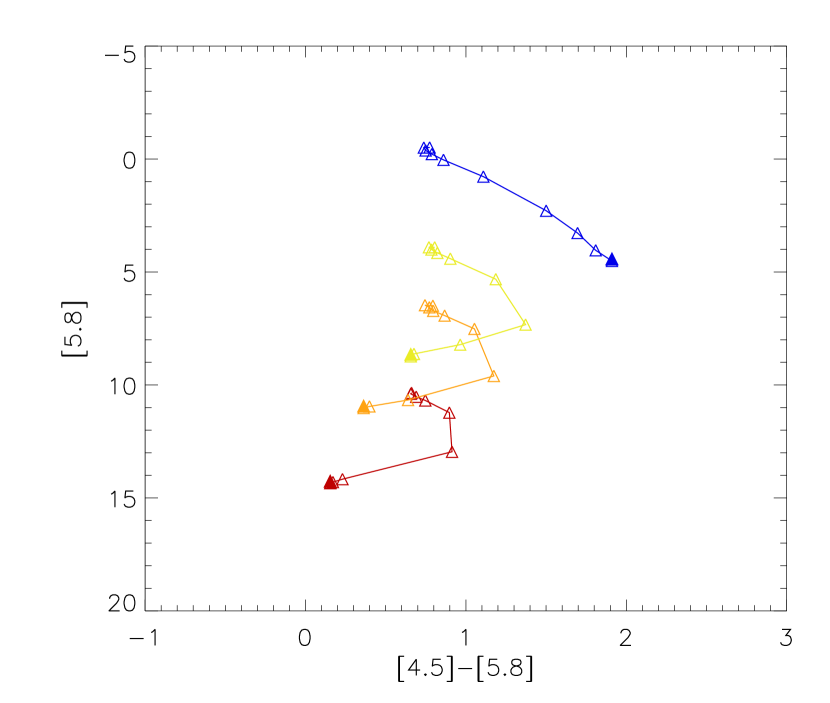
Figure 7: Color-magnitude plot for the four Class I models with fluxes integrated over a 3000 AU radius aperture. The symbol colors are as described in Figure 6. The higher temperature sources are more luminous (except for the edge-on sources in some cases). Magnitudes are scaled to a distance of 2 kpc.

We use a 3-D Monte Carlo Radiative transfer code described in Paper I, which uses the radiative equilibrium method developed by Bjorkman & Wood (2001). The geometries considered in this paper are 2-D so we use a 2-D grid ($r-\theta$). The model geometries consist of a stellar source, a flared accretion disk, and a rotationally-flattened infalling envelope (Ulrich 1976; Terebey, Shu & Cassen 1984) with partially-evacuated bipolar cavities (Papers I & II). The envelope density decreases via a power-law at large radii ($\rho\propto r^{-1.5}$) and then merges with the ambient density of the surrounding molecular cloud. Luminosity is generated by the central star and accretion in the disk. This radiation is scattered and reprocessed by the surrounding circumstellar dust. We note that we solve for the 3-D temperature in any specified circumstellar geometry; therefore we naturally compute a hot surface on the inner disk wall as shown in Figure 1, as we have in all our previous publications using these models (e.g., Wood et al. 2002a,b, Papers I & II, Rice et al. 2003, Walker et al. 2004). In addition, our cavity dust is hot and has a high emissivity, despite its low density (Paper I, Figure 7). Therefore our Class 0-II models include mid-IR thermal emission from the warm disk and cavity regions, in addition to any envelope component. Our models also accurately compute scattering and polarization using arbitrary scattering phase functions. Our models conserve flux absolutely (that is, to 0%). The primary source of error in our models is photon counting statistics (and, when comparing to data, knowledge of the appropriate input circumstellar geometry and dust properties). Running more photons produces higher signal-to-noise spectra. The models produced for this paper took 3 hours each to run (on 2 GHz PCs running g77). The exiting photons were binned into 10 inclinations and 200 frequencies to produce SEDs.

2.1.1 Dust Properties and Dust Sublimation Radius

We use similar grain properties as in Paper II (Table 3): a large-grain model for the high-density regions in the disk (Wood et al. 2002b); a medium-sized grain model for the upper layers of the disk (Cotera et al. 2001); and for the envelope and cavity, a grain model that gives an extinction curve typical of molecular clouds with $r_{V}$, the ratio of total-to-selective extinction, equal to 4.3. The dust sublimation temperature is chosen to be 1600 K.

The disk dust sublimation radius was calculated through iteration by running the code several times and setting the opacity to be zero in grid cells when the temperature rises above $T_{sub}$. In the final iteration, there are no cells with $T>T_{sub}$ (Walker et al. 2004). We determined an empirical formula that fit our range of stellar temperatures:

$$R_{sub}/R_{\star}=(T_{sub}/T_{\star})^{-2.085}.$$ (1)

This is very similar to the optically thick blackbody radiative equilibrium temperature, $r\propto T^{-2}$, and thus likely has little dependence on the dust opacity law, unlike the optically thin radiative equilibrium limit (Lamers & Cassinelli, 1999; Beckwith et al., 1990). This behavior is obviously due to the fact that the inner disk wall is opaque at all wavelengths; this is true over a wide range of disk masses (Wood et al. 2002b).

2.2 Homologous Models

We start by specifying a Class I model for a low-mass (0.5 M_☉) YSO, based on previous observations and models (Kenyon et al. 1993a,b, Whitney et al. 1997, Lucas & Roche 1997, 1998; Padgett et al. 1999). Then we will scale this model homologously for different stellar temperatures. To construct a homologous model, we require that the inner and outer radii be scaled to the dust destruction radius and that the optical depths (at a given inclination angle) be the same for all the models (Ivezić & Elitzur 1997; Carciofi et al. 2004). This will result in a homologous temperature distribution for the circumstellar dust, and the shape of the thermal contribution to the SED will be invariant (only scaled by the increased luminosity). Table 1 shows the model parameters that result. For all the models we choose the inner radius to be the dust destruction radius. For the low-mass model, the outer radius is 3000 AU (chosen to be as small as reasonable since the high temperature model will be huge). The disk radius and envelope centrifugal radius is 300 AU, and the envelope infall rate is $6.7\times 10^{-6}$ M_☉/yr. The model includes a flared disk of mass 0.01 $M_{\sun}$. The ratio of disk scale height to radius at the disk outer radius is $h/r=0.12$ (chosen to match the HH30 disk, Burrows et al. 1996; Wood et al. 1998). For simplicity in comparing models, we set the disk accretion rate to 0, so the disk radiates from thermal reprocessing of starlight only. The bipolar cavity has a curved shape ($z=a(x^{2}+y^{2})^{b}$, where $b=1.5$ and $a$ is set by the opening angle) and an opening angle of 20 degrees at the outer radius. The bipolar cavity is filled with constant-density dust with an optical depth along the polar direction of $\tau_{V}=5$ at V (0.55 $\mu$m). Because the low-$T_{\star}$ models have smaller outer envelope radii, they have correspondingly higher density in the bipolar cavities. Based on these parameter choices, the optical depth through the envelope at an inclination of 60 degrees is $\tau_{V}$=25; and through the disk midplane is $\tau_{V}$=193,000.

The parameters for the other models are then chosen to give the same inner and outer radii scaled to dust destruction radius, and the same optical depths at 0°(cavity), 60°(envelope), and 90°(disk). Thus the envelope and disk masses and radii grow with the higher $T_{\star}$ models, as shown in Table 1. We choose stellar parameters appropriate for young stars of age $3\times 10^{5}$ yrs (Siess, Dufour, & Forestini, 2000).

Figure 2 shows SEDs for the homologous model. Figure 2a shows only the thermal spectrum from each model, and does not include the stellar direct or scattered radiation. From this we can see that the shapes of the spectra are similar for all models. The temperature structure and therefore thermal emission is determined only by the luminosity of the incident radiation (which sets the dust destruction radius) and where the radiation is absorbed (determined by geometry and density). The slight differences between the models are due to the fact that the models are not perfectly homologous for two main reasons: 1) The geometries are slightly different between the models because the ratio of the stellar size to dust destruction radius varies: In the high-$T_{\star}$ models, the star is effectively a point source, and in the low-$T_{\star}$ models it is larger than the inner disk wall height; and 2) Because the dust scattering albedo is non-zero and varies with wavelength, the total absorbed luminosity varies slightly between the models (i.e., the dust scattering albedo at the wavelengths where most of the stellar flux is emitted is lower in the low-$T_{\star}$ models than the high-$T_{\star}$ models so a slightly higher fraction of flux is absorbed in the low $T_{\star}$ models). However, the differences are slight and they do not detract from the main point, that the thermal spectra are similar between the models.

Figure 2b shows the total spectrum from each model. Here we see that the stellar contribution (scattered and direct) is greater in the low-$T_{\star}$ models. Thus, compared to the high-$T_{\star}$ models, the spectrum is relatively blue. We emphasize that the high-temperature models are redder in the 1-10 $\mu$m region, not because the envelope mass is larger but because the spectrum in this region is a more pure thermal spectrum. Note also that one reason the thermal spectra are similar for all the models is that the dust sublimation temperature $T_{sub}$ sets the cutoff for the maximum temperature of the thermal radiation. Thus the peak of the thermal emission occurs at the same wavelength for all the models. If there were no cutoff with $T_{sub}$, then the high $T_{\star}$ sources would have a more continuous blend between stellar and thermal spectra.

2.3 Class I Models guided by observations

The high-$T_{\star}$ models in Figures 2 are not realistic, given the homologous scaling of the disk parameters from the low-$T_{\star}$ disk. Here we show more realistic geometries gleaned from previous observations and modeling of high-mass sources (e.g. Alvarez, Hoare, & Lucas, 2004; Beltrán et al., 2004; Beuther et al., 2004; Sandell & Sievers, 2004; Sandell, 2000; Shepherd, Claussen, & Kurtz, 2001). We keep the envelope optical depths similar between the models to help understand the comparisons between the models better. The model parameters are shown in Table 2. The main difference between these and the homologous model is in the disk parameters. Like the homologous models, the disk inner radii are set to the dust sublimation radius, $R_{sub}$. The outer radii are chosen based on observations cited above. The disk masses are chosen to be 5% of the stellar mass. The disk scale heights are calculated at $R_{sub}$ from the analytic solution of the hydrostatic equation assuming the disk temperature is vertically isothermal. Since the disk temperature is known at $R_{sub}$, it is straightforward to calculate the scale height $h$ at this location (equal to the sound speed divided by the Keplerian velocity; Bjorkman 1997). The gaussian scale height at each radius is then $h=h_{sub}(r/R_{sub})^{1.25}$. Disk accretion is included, but the effect on the SED is minor since the disk accretion luminosity is relatively small for all of the models (Table 2). The outer envelope radii are left large since the hotter stars will heat up surrounding ambient material out to several pc. Note that the envelope masses of the high-$T_{\star}$ models are large due to the large outer radii. However, the relevant parameter for the radiative transfer is optical depth, which is similar between the models. Therefore the variation of the thermal emission is due to circumstellar geometry.

Figure 3a shows that hotter $T_{\star}$ models have relatively more $1-10\mu$m thermal emission than the cooler $T_{\star}$ models. This is due to the larger inner disk walls in the high-$T_{\star}$ models as a result of the larger dust destruction radius ($h/r$ at $R_{sub}$ in Table 2). This is similar to the “puffed-up” inner disk region invoked by Natta et al. (2001) to explain the SEDs of Ae/Be stars. The wall intercepts and reprocesses radiation near the dust sublimation temperature $T_{sub}$ with its peak radiation at about 2 $\mu$m. This effect did not appear in the homologous model because $h/r$ at $R_{sub}$ was the same in all the models (Table 1). The increased $1-10\mu$m emission in the high-$T_{\star}$ models is counteracted slightly when the stellar emission is included (Figure 3b) but for the models with $T_{\star}>8000$K, the colors are bluer towards pole-on inclinations and higher $T_{\star}$ due to emission from the disk wall. This figure shows that the disk structure and emission properties affect the 1-10$\mu$m spectrum in Class I sources. Note that the SEDs in Figs. 3a and 3b include the flux from the entire envelope which extends to nearly 2 pc in the case of the hot star model (Table 1). Figure 3c shows the results integrated in a 3000 AU radius aperture (1.5″at a distance of 2 kpc), more typical of aperture photometry observations. In this case, the hottest $T_{\star}$ model has less short- and long-wave flux in the smaller aperture giving a more rounded SED shape. It is rather striking that the SEDs of these four Class I models, with nearly identical optical depths in the cavity and envelope, have such different shapes.

2.4 Other Evolutionary States: Class 0 and II

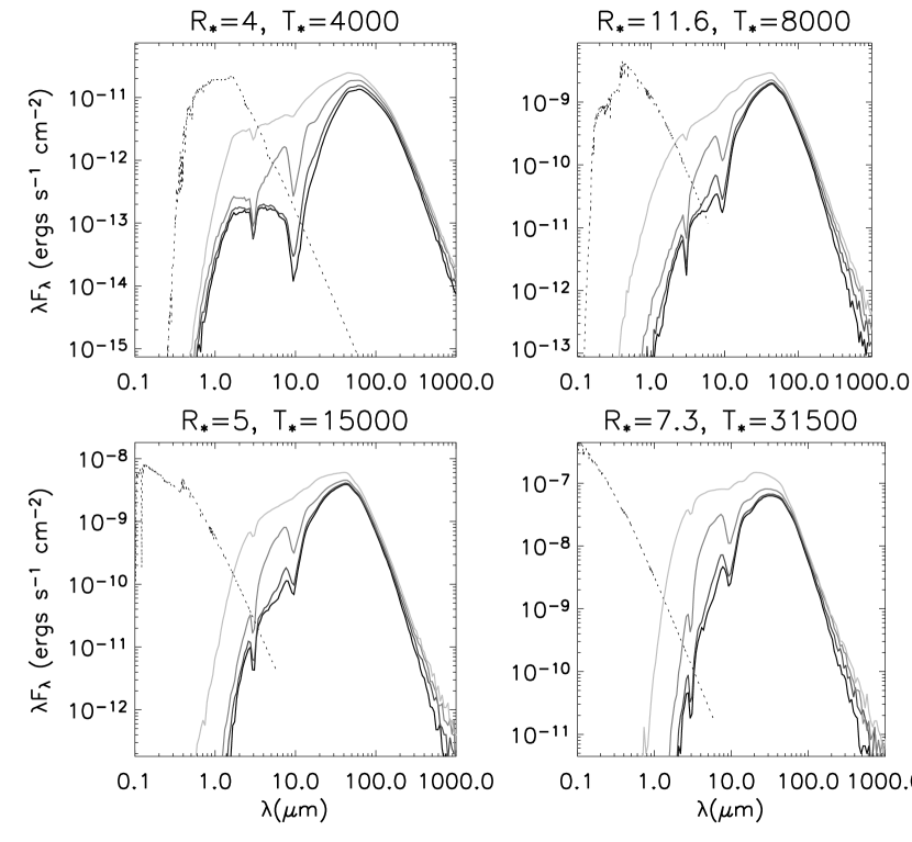
Figure 4: Class 0 SEDs (Table 3). The total spectrum (stellar direct+scattered and thermal) is plotted for each stellar temperature. Inclination variations are as in Figure 1. Fluxes are scaled to a distance of 2 kpc. The spectra are integrated over 3000 AU radius apertures from the central source.

To see how stellar temperature affects other evolutionary states, we also show SEDs of Class 0 and II sources for the four stellar temperatures. We keep the stellar parameters the same for the Class 0 and II models even though they would obviously evolve over this time period. However, this allows us to isolate better the differences between the resulting SEDs (e.g., the disk scales heights will be similar if the stellar properties do not change). Figure 4 shows SEDs for Class 0 sources with the model parameters in Table 3. The envelope optical depths are four times higher than the Class I model, and the polar optical depths are two times higher. The disk radii are smaller and disk masses higher (0.1 times the stellar mass), giving larger midplane optical depths. The SEDs are shown integrated in a 3000 AU aperture. Except for the pole-on inclinations, these show a trend for the high-$T_{\star}$ models to have redder $1-10\mu$m colors. As in the Class I models, the disk walls contribute more radiation at 2-10$\mu$m in the high-$T_{\star}$ models but this is only apparent towards pole-on inclinations ($i<45$°).

Class II SEDs are shown in Figure 5 with the model parameters in Table 4. The disk parameters are similar to the Class I models except that the masses are lower, since they are more evolved. At a wavelength range of 1-2$\mu$m, there is a tendency for the models to become more red with increasing $T_{\star}$. At 2 $\mu$m the disk emission kicks in and the larger walls from the high-$T_{\star}$ models show a blue spectrum towards pole-on inclinations from $2-10\mu$m. However, the edge-on inclinations are red or flat in the models due to obscuration by the flaring outer regions. Thus when inclination is included, there is again a large spread in colors at $1-10\mu$m. We note that the disk models do not include the effect of gas opacity inside the dust destruction radius. This should not be a problem in the low mass disks due to low opacities (Lada & Adams 1992) but it may be important in the high-mass disks. In addition, PAH emission is likely an important contributor in the high-$T_{\star}$ models. This is beyond the scope of this paper and will be explored in the future.

2.5 Color-color and Color-magnitude diagrams

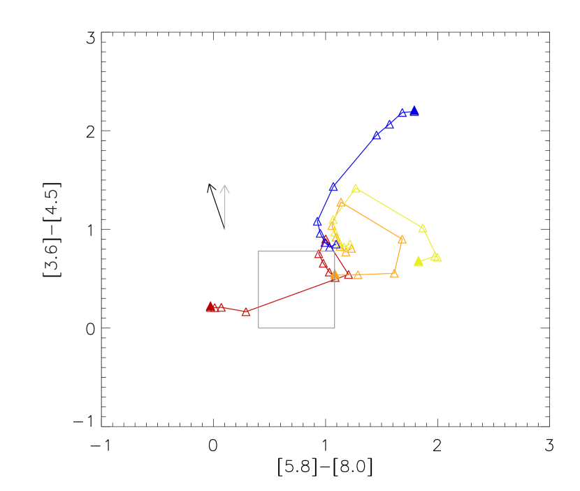
Figure 6: Color-color plot ([5.8]-[8.0] vs. [3.6]-[4.5]) of the four Class I models with fluxes integrated over a 3000 AU radius aperture. The different colors are for the different stellar temperatures (red: T=4000 K; orange: T=8000 K; yellow: T=16000 K; blue: T=31500 K). For each model, 10 inclinations ranging from edge-on to pole-on are plotted. The filled symbols show the edge-on colors. The grey box is a region denoted by Allen et al. (2004) as the approximate domain of Class II sources. The black arrow denotes the reddening vector for the diffuse ISM (Cardelli, Clayton, & Mathis 1989), and the grey arrow is derived from GLIMPSE data (Indebetouw et al. 2004). The length of the arrows represent A${}_{V}=30$.

Figure 6 shows color-color plots in the IRAC bands [3.6]-[4.5] vs. [5.8]-[8.0] for the Class I models (§2.3 and Table 2) integrated in a 3000 AU radius aperture. There is a trend for the high-$T_{\star}$ models to be more red, though there is overlap due to the broad spread in inclination within a model. The color range of these Class I models (with similar optical depths) spans the range of observations in the four star forming clusters presented by Allen et al. (2004)! The grey box in Figure 6 shows the region denoted by Allen et al. as the approximate domain of Class II sources. Some of edge-on Class I models are blueward of this domain (see Figure 3c). Figure 7 shows a color-magnitude diagram for the Class I models. This shows some spread in both magnitude and color with each model but a general trend for the high-$T_{\star}$ models to be brighter (obviously) and more red. The Class I models in Figure 6 can be compared to those presented by Allen et al. (2004) in their Figure 1. Their models show a trend for higher luminosity sources to be more red in [5.8]-[8.0] and higher density envelopes (presumably younger sources) to be more red in [3.6]-[4.5]. It is not clear if they varied stellar temperature in their Class I models, but our models show a similar trend for higher luminosity sources to have redder [3.6]-[4.5] colors due to stellar temperature effects. The main difference however is that our models in general give bluer colors for the same envelope parameters (density or infall rate) due to our inclusion of partially evacuated bipolar cavities and flared disks in the Class I models (Paper I, Figure 12). Thus we would likely estimate a younger evolutionary state (higher density envelope) for a given set of observational colors.

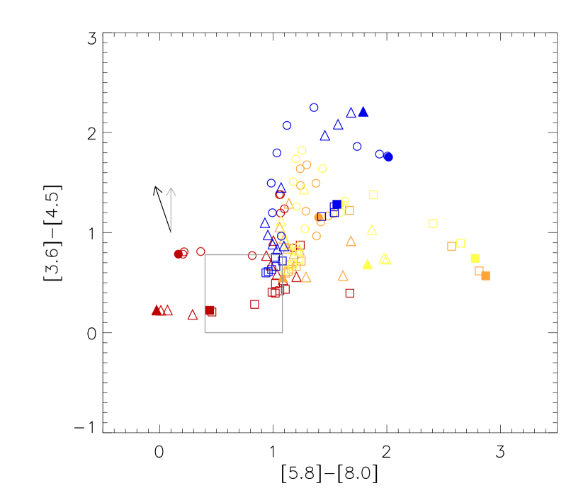
Figure 8: Color-color plot including Class 0 and Class II sources in addition to the Class I sources shown in Fig. 6. The different colors represent the different stellar temperatures (red: T=4000 K; orange: T=8000 K; yellow: T=16000 K; blue: T=31500 K). The symbols represent the three evolutionary states (circles: Class 0; triangles: Class I; boxes: Class II). For each model, 10 inclinations are plotted ranging from edge-on to pole-on in equal intervals of $\cos i$. The filled symbols show the edge-on sources. The grey box is a region denoted by Allen et al. (2004) as the approximate domain of Class II sources. There is a slight trend with higher temperature sources being more red, especially in [3.6]-[4.5]. Notice that five reddest sources in [5.8]-[8.0] are Class II sources. The eight bluest source in [5.8]-[8.0] are Class 0 and I sources. The arrows represent reddening vectors with A${}_{V}=30$ as described in Figure 6.

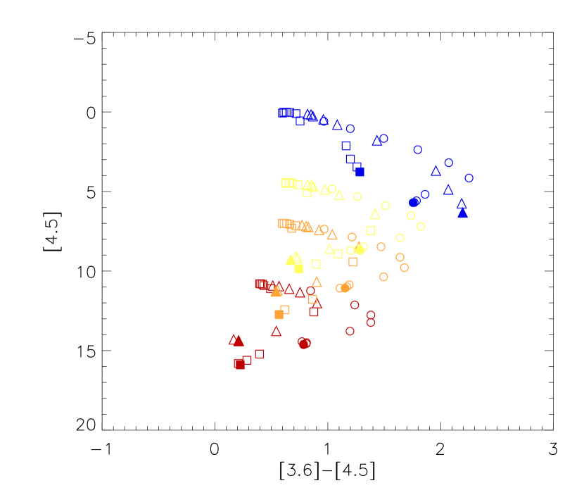
Figure 9: Color-magnitude plot for all evolutionary states and inclinations. The symbols are as described in Fig. 8. Magnitudes are scaled to a distance of 2 kpc. For a given stellar temperature, the [3.6]-[4.5] color generally shows the expected behavior with evolutionary sequence with the Class II sources at left and Class 0 sources at right (with exceptions).

Finally, we show color-color and color-magnitude plots in Figures 8 and 9 adding in Class 0 and Class II sources. There are several interesting things to note in Fig. 8: the six reddest sources in [5.8]-[8.0] are Class II sources (with stellar temperatures 8000 and 15000 K). The eight bluest sources in [5.8]-[8.0] are Class 0 and I sources (with $T_{\star}=4000$ K). This is backwards from the common wisdom. The [3.6]-[4.5] color behaves more as expected with Class 0-I sources most red and Class I-II sources most blue. There is somewhat of a dearth of sources in the “Class II domain” of Allen et al. (2004) (the grey box). This is due to the fact that we computed only one cool-$T_{\star}$ disk model, whereas most T Tauri stars in a low-mass cloud are likely cool with a range of disk masses. Allen et al.’s disk models all used a stellar temperature of 4000 K and inclinations of 30°and 60°. Both the hottest and coolest of our disk models fall at the right edge of their Class II domain region. The mid-temperature disks lie just to the right for most inclinations and then to the far right for the partially obscured (near edge-on) sources. Most of the Class 0 sources fall in the color range of 1-2 in both [5.8]-[8.0] and [3.6]-[4.5]. The Class I sources, on the other hand, span nearly the entire range of the plot. They suffer the most variation due to inclination, stellar temperature, inner disk wall, and scattered light effects. And Class II and 0 sources can be found at unexpected locations in the color-color plot as well, albeit with lower frequency.

Figure 9 shows a more systematic behavior in the color-magnitude plot. The hotter $T_{\star}$ sources tend to be brighter, and within a given flux range, their colors follow an evolutionary sequence with bluer colors being younger. Thus, the color-magnitude plot provides some guidance in separating stellar temperature effects from evolutionary effects.

3 Conclusions

In this series of papers, we have shown that inclination effects, aperture size, scattered light, and stellar temperature cause a broad spread in the colors of a source at a single evolutionary state. There is systematic behavior, as shown in the color-magnitude diagrams (Fig. 9), but the behavior is not as simple as using the slope of the observed SED (or the IRAC [3.6]-[4.5] vs. [5.8]-[8.0] color-color plot) to estimate evolutionary state (Fig. 8) for a given source. There are trends in color space that could be applied in a statistical sense to a cluster. More modeling than the small grid presented here would be useful to provide a statistical guide for interpreting mid-IR color-color plots. Our codes are now publicly available and we are in the process of computing a large grid of models which will also be publicly available.

We note that these problems for interpreting evolutionary state based on SEDs are also reduced if long wavelength ($\lambda>100\mu$m) observations are obtained. These are much less sensitive to geometry (and inclination) and thus 1-D or simple disk models do a reasonable job estimating circumstellar mass and hence evolutionary state, assuming younger sources have more massive circumstellar envelopes (e.g., Mueller et al. 2002). Also, if the temperature of the stellar source can be estimated, the problems of interpreting the mid-IR colors in terms of evolutionary state become less severe. The stellar contribution can be estimated at wavelengths shortward of 2$\mu$m where disk emission does not contribute. In our preliminary modeling of the Spitzer IRAC data in the giant H II region RCW 49 (Whitney et al. 2004), we find that we can estimate the stellar temperature by fitting multi-band photometry across the $1-10\mu$m range (2MASS JHK and the four IRAC bands). This improves our ability to simultaneously estimate the evolutionary state and central source temperature. We will present these results in our next paper.

Table 1: Homologous Models

Stellar Temperature:	4000	8000	15000	31500
Envelope infall rate ($/10^{-5}M_{\sun}/$yr)	0.67	10.5	10	49
Envelope mass ($M_{\sun}$)	0.12	18	46	2150
Stellar radius ($R_{\sun}$)	4	11.6	5	7.3
Stellar luminosity ($L_{\sun}$)	3.67	494	1134	46900
Stellar mass ($M_{\sun}$)	0.5	6.0	6.2	20
Envelope & Disk inner radius ($R_{\star}$)	6.7	29	106	500
Envelope & Disk inner radius (AU)	0.125	1.55	2.47	16.9
Envelope outer radius (AU)	3000	36900	59000	404000
Disk mass ($M_{\sun}$)	0.01	1.28	3.06	138
Disk outer radius (AU)	300	3691	5900	40400
$h/r$ at $R_{\star}$	0.011	0.0074	0.0053	0.0036
$h/r$ at $R_{sub}$	0.017	0.017	0.017	0.017
Cavity opening angle (°)	20	20	20	20
Cavity density ($/10^{-20}$ gm cm-3)	37	3.0	1.9	0.28
$\tau_{V}$ ($i=0$°)	5	5	5	5
$\tau_{V}$ ($i=60$°)	25	25	25	25
$\tau_{V}$ ($i=90$°, $/10^{5}$)	1.93	1.93	1.93	1.93

Note. — Inner Envelope/Disk radii are set to the dust sublimation radius, $R_{sub}$.

Table 2: Class I Models

Stellar Temperature:	4000	8000	15000	31500
Envelope infall rate ($/10^{-5}M_{\sun}/$yr)	0.67	3.8	4.8	22
Envelope mass ($M_{\sun}$)	0.12	8.5	31	1430
Disk mass ($M_{\sun}$)	0.02	0.30	0.31	1
Disk accretion rate ($/10^{-8}M_{\sun}/$yr)	2.1	24	24	120
Disk accretion luminosity ($/10^{-4}L_{acc}/L_{\star}$)	17	1.4	0.38	0.022
Disk outer radius (AU)	300	400	500	500
$h/r$ at $R_{\star}$	0.025	0.018	0.016	0.016
$h/r$ at $R_{sub}$	0.041	0.041	0.051	0.074
Cavity density ($/10^{-20}$ gm cm-3)	37	3.0	1.9	0.28
$\tau_{V}$ ($i=90$°, $/10^{5}$)	1.63	1.77	0.80	0.28

Note. — Only parameters different from Table 1 are listed here.

Table 3: Class 0 Models

Stellar Temperature:	4000	8000	15000	31500
Envelope infall rate ($/10^{-5}M_{\sun}/$yr)	0.88	5.2	6.1	25
Envelope mass ($M_{\sun}$)	0.15	11.5	58	2700
Disk mass ($M_{\sun}$)	0.05	0.60	0.62	2
Disk accretion rate ($/10^{-8}M_{\sun}/$yr)	32	250	250	1400
Disk accretion luminosity ($/10^{-4}L_{acc}/L_{\star}$)	251	14	4.0	0.25
Disk outer radius (AU)	50	80	100	100
$h/r$ at $R_{\star}$	0.025	0.018	0.016	0.016
$h/r$ at $R_{sub}$	0.040	0.041	0.051	0.074
Cavity density ($/10^{-20}$ gm cm-3)	74	6.05	3.8	0.55
Cavity opening angle (°)	10	10	10	10
$\tau_{V}$ ($i=0$°)	10	10	10	10
$\tau_{V}$ ($i=60$°)	100	100	100	100
$\tau_{V}$ ($i=90$°, $/10^{5}$)	25	18.6	7.9	2.87

Note. — Only parameters different from Table 1 are listed here.

Table 4: Class II Models

Stellar Temperature:	4000	8000	15000	31500
Disk mass ($M_{\sun}$)	0.01	0.15	0.15	1
Disk accretion rate ($/10^{-8}M_{\sun}/$yr)	1.1	12	12	59
Disk accretion luminosity ($/10^{-4}L_{acc}/L_{\star}$)	8.3	0.68	0.19	0.001
Disk outer radius (AU)	300	400	500	500
$h/r$ at $R_{\star}$	0.025	0.018	0.016	0.016
$h/r$ at $R_{sub}$	0.041	0.041	0.051	0.074
$\tau_{V}$ ($i=90$°$/10^{5}$)	0.82	0.89	0.39	0.14

Note. — Only parameters different from Table 1 are listed here. The envelope infall rate is 0.

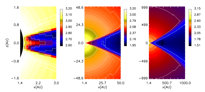
Figure 1: 2-D temperature structure of a Class I source (Table 2, with $T_{\star}$ equal to 8000 K) on three different size scales. The small-scale plot (left) shows the hot cavity, the hot inner disk wall and surface, and the effect of accretion heating up the midplane at small radii. The black region at left is the region inside the dust destruction radius. On larger scales (right panel), we can see the shadowing in the equatorial plane caused by the opaque disk. The color bars show log of the temperature. The contours correspond to the labeled values on the color bars.

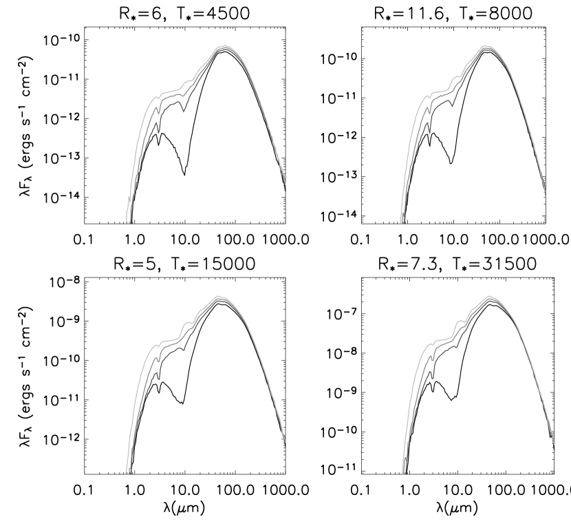
Figure 2a: SEDs of the four homologous models. Four inclinations are plotted: $\cos i=0.05$ (edge-on), 0.35, 0.65, 0.95 (pole-on). Inclination variations are shown with different shades of grey from light grey (pole-on) to black (edge-on). Fluxes are scaled to a distance of 2 kpc. (a) The thermal spectrum only. (b) total spectrum, including stellar direct+scattered flux and thermal. The input stellar spectrum is shown as a dotted black line.

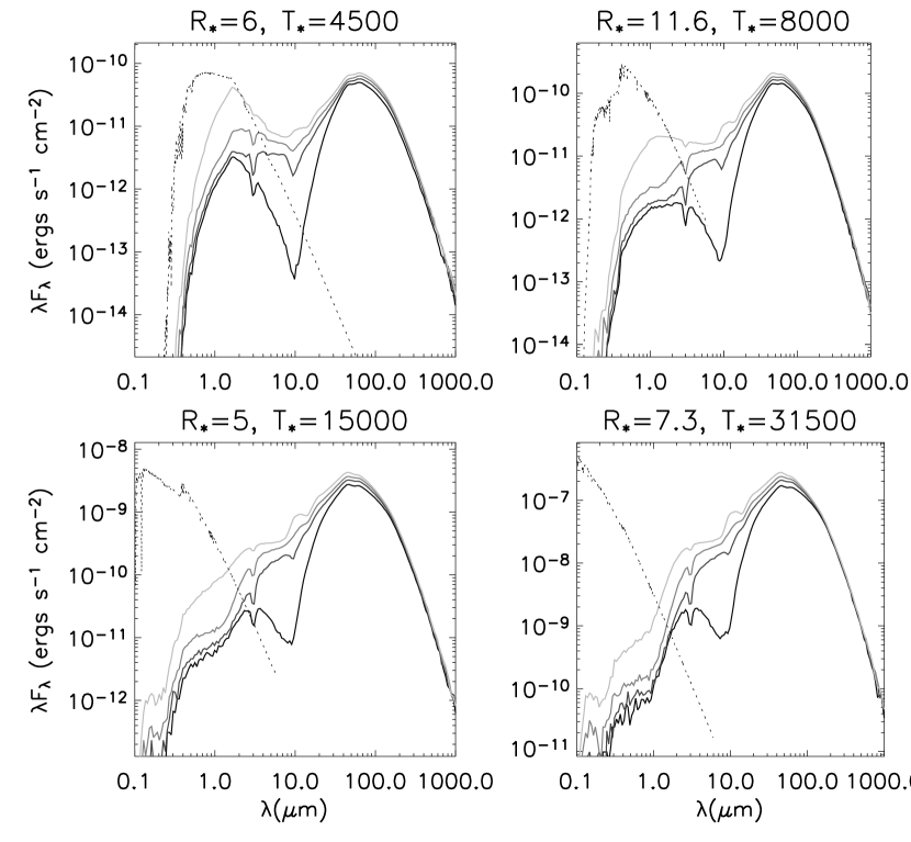
Figure 2b:

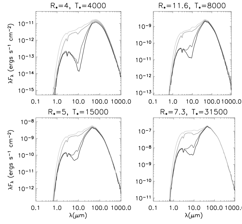
Figure 3a: SEDs of the four Class I models. Inclinations are the same as Fig. 1. Fluxes are scaled to a distance of 2 kpc. (a) The thermal spectrum only. (b) total spectrum, including stellar direct+scattered flux and thermal. The input stellar spectrum is shown as a dotted black line. (c) the spectrum integrated in 3000 AU radius apertures (1.5″radius aperture at 2000 pc distance).

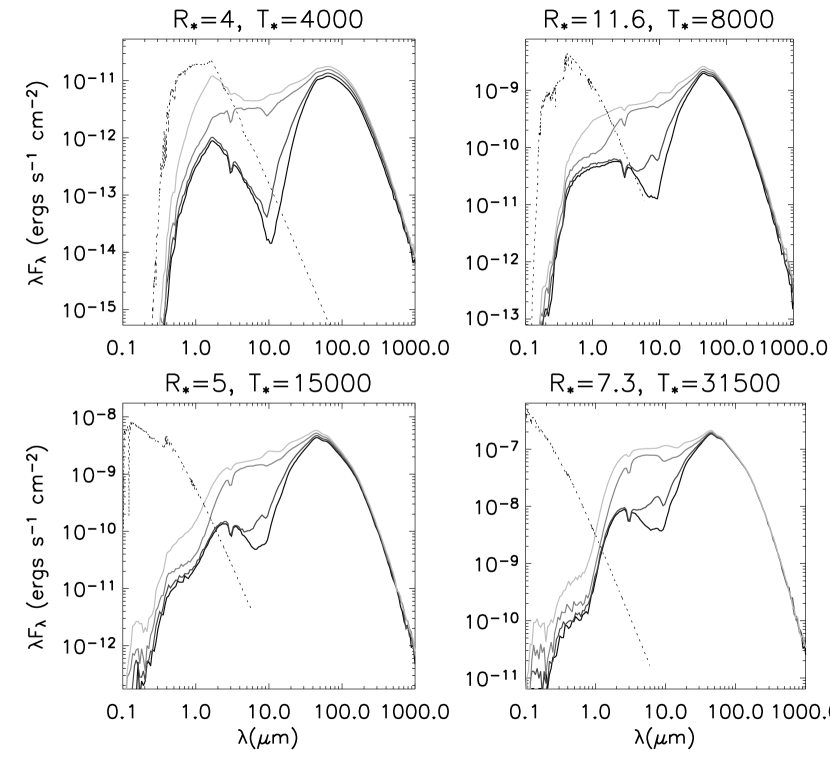
Figure 3b:

Figure 3c:

Figure 5: Class II SEDs (Table 4). The total spectrum (stellar direct+scattered and thermal) is plotted for each stellar temperature. Inclination variations are as in Figure 1. Fluxes are scaled to a distance of 2 kpc.

References

- Allen et al. (2004) Allen, L. E., et al. 2004, ApJS, 154, 363
- Alvarez, Hoare, & Lucas (2004) Alvarez, C., Hoare, M., & Lucas, P. 2004, A&A, 419, 203
- André et al. (1993) André, P., Ward-Thompson, D., & Barsony, M. 1993, ApJ, 406, 122
- Beckwith et al. (1990) Beckwith, S. V. W., Sargent, A. I., Chini, R. S., & Gusten, R. 1990, AJ, 99, 924
- Behrend & Maeder (2001) Behrend, R. & Maeder, A. 2001, A&A, 373, 190
- Beltrán et al. (2004) Beltrán, M. T., Cesaroni, R., Neri, R., Codella, C., Furuya, R. S., Testi, L., & Olmi, L. 2004, ApJ, 601, L187
- Beuther et al. (2004) Beuther, H., et al. 2004, ArXiv Astrophysics e-prints, astro-ph/0402505
- Bjorkman (1997) Bjorkman, J. E. 1997, in Stellar Atmospheres: Theory and Observations, ed J.P. De Greve, R. Blomme, and H. Hensberge (New York:Springer), 239
- Bjorkman & Wood (2001) Bjorkman, J. E., & Wood, K. 2001, ApJ, 554, 615
- Bonnell, Bate, & Zinnecker (1998) Bonnell, I. A., Bate, M. R., & Zinnecker, H. 1998, MNRAS, 298, 93
- Burrows et al. (1996) Burrows, C. J., et al. 1996, ApJ, 473, 437
- Cardelli, Clayton, & Mathis (1989) Cardelli, J. A., Clayton, G. C., & Mathis, J. S. 1989, ApJ, 345, 245
- Carciofi et al. (2004) Carciofi, A. C., Bjorkman, J. E., & Magalh es, A. M. 2004, ApJ, 604, 238
- Cotera et al. (2001) Cotera, A., Whitney, B. A., Young, E., Wolff, M. J., Wood, K., Povich, M., Schneider, G., Rieke, M., & Thompson, R. 2001, ApJ, 556, 958
- Fazio et al. (2004) Fazio, G. G. et al., 2004, ApJS, 154, 10
- Gómez et al. (1997) Gómez, M., Whitney, B. A., & Kenyon, S. J. 1997, AJ, 114, 265
- Indebetouw et al. (2004) Indebetouw, R. et al. 2004, ApJ, submitted
- Ivezić & Moshe (1997) Ivezić, Z. & Elitzur, M. 1997, MNRAS, 287, 799
- Kenyon et al. (1993a) Kenyon, S. J., Calvet, N., & Hartmann, L. 1993a, ApJ, 414, 676
- Kenyon et al. (1993b) Kenyon, S. J., Whitney, B., Gómez, M., & Hartmann, L. 1993b, ApJ, 414, 773
- Kenyon & Hartmann (1995) Kenyon, S. J. & Hartmann, L. 1995, ApJS, 101, 117
- Lada (1987) Lada, C. J. 1987, in Star Forming Regions, edited by M. Peimbert & J. Jugaka (Dordrecht, Reidel), 1
- Lada & Adams (1992) Lada, C. J. & Adams, F. C. 1992, ApJ, 393, 278
- Lada (1999) Lada, C. J. 1999, in The Origin of Stars and Planetary Systems, edited by C. J. Lada & N. D. Kylafis (Kluwer: Dordrecht), 143
- Lamers & Cassinelli (1999) Lamers, H. J. G. L. M. & Cassinelli, J. P. 1999, in Introduction to Stellar Winds, (Cambridge: Cambridge University Press), 163
- Lucas & Roche (1997) Lucas, P. W., & Roche, P. F. 1997, MNRAS, 286, 895
- Lucas & Roche (1998) Lucas, P. W., & Roche, P. F. 1998, MNRAS, 299, 699
- Maeder & Behrend (2002) Maeder, A. & Behrend, R. 2002, Ap&SS, 281, 75
- Megeath et al. (2004) Megeath, S. T., et al. 2004, ApJS, 154, 367
- Mueller et al. (2002) Mueller, K. E., Shirley, Y. L., Evans, N. J., II, Jacobson, H. R. 2002, ApJs, 143, 469
- Muzerolle et al. (2004) Muzerolle, J., et al. 2004, ApJS, 154, 379
- Natta et al. (2001) Natta, A., Prusti, T., Neri, R., Wooden, D., Grinin, V. P., & Mannings, V. 2001, A&A, 371, 186
- Padgett et al. (1999) Padgett, D. L., Brandner, W., Stapelfeldt, K. R., Strom, S. E., Terebey, S., & Koerner, D. 1999, AJ, 117, 1490
- Reach et al. (2004) Reach, W. T., et al. 2004, ApJS, 154, 385
- Reipurth et al. (2000) Reipurth, B., Yu, K. C., Heathcote, S., Bally, J., & Rodríguez, L. F. 2000, ApJ, 120, 1449
- Rice et al. (2003) Rice, W. K. M., Wood, K., Armitage, P. J., Whitney, B. A., & Bjorkman, J. E. 2003, MNRAS, 342, 79
- Richer et al. (2000) Richer, J. S., Shepherd, D. S., Cabrit, S., Bachiller, R., & Churchwell, E. 2000, in Protostars and Planets IV, eds. V. Mannings, A. P. Boss, S. R. Russell (Tucson: University of Arizona Press), p. 867
- Rieke et al. (2004) Rieke, G. H. et al. 2004, ApJS, 154, 25
- Sandell (2000) Sandell, G. 2000, A&A, 358, 242
- Sandell & Sievers (2004) Sandell, G. & Sievers, A. 2004, ApJ, 600, 269
- Shepherd, Claussen, & Kurtz (2001) Shepherd, D. S., Claussen, M. J., & Kurtz, S. E. 2001, Science, 292, 1513
- Siess, Dufour, & Forestini (2000) Siess, L., Dufour, E., & Forestini, M. 2000, A&A, 358, 593
- Terebey et al. (1987) Terebey, S., Shu, F. H., & Cassen, P. 1984, ApJ, 286, 52
- Ulrich (1976) Ulrich, R. K. 1976, ApJ, 210, 377
- Walker et al. (2004) Walker, C., Wood, K., Lada, C. J., Robitaille, T., Bjorkman, J. E., & Whitney, B. 2004, MNRAS, 351, 607
- Werner et al. (2004) Werner, M. W. et al. 2004, ApJS, 154, 1
- Whitney, Kenyon, & Gómez (1997) Whitney, B. A., Kenyon, S. J., & Gómez, M. 1997, ApJ, 485, 703
- Whitney et al. (2003) Whitney, B. A., Wood, K., Bjorkman, J. E., & Wolff, M. J. 2003a, ApJ, 591, 1049 (Paper I)
- Whitney et al. (2003) Whitney, B. A., Wood, K., Bjorkman, J. E., & Cohen, M. 2003b, ApJ, 598, 1099 (Paper II)
- Whitney et al. (2004) Whitney, B. A., et al. 2004, ApJS, 154, 315
- Wood et al. (1998) Wood, K., Kenyon, S. J.; Whitney, B., & Turnbull, M. 1998, ApJ, 497, 404
- Wood et al. (2002a) Wood, K., Wolff, M. J., Bjorkman, J. E., & Whitney, B. 2002a, ApJ, 564, 887
- Wood et al. (2002b) Wood, K., Lada, C. J., Bjorkman, J. E., Kenyon, S. J., Whitney, B., & Wolff, M. J. 2002b, ApJ, 567, 1183