Pure Luminosity Evolution Models: Too Few Massive Galaxies at Intermediate and High Redshift

Abstract

We compare pure luminosity evolution (PLE) models with recent data at low and high redshift. These models assume that massive galaxies were assembled and formed most of their stars at high redshift ($z>3$) and have evolved without merging or substantial dust obscuration since then. Our models span the full range of plausible metallicities, initial mass functions (IMF’s) and star formation histories. We require them to reproduce the abundance of galaxies by colour and luminosity in the Sloan Digital Sky Survey and we investigate whether they can simultaneously fit (i) the observed galaxy counts as a function of redshift in magnitude limited surveys with $K<20$, and (ii) the colour and $M/L$ ratio evolution of red sequence galaxies in clusters. All models that are consistent with (ii) predict galaxy counts at $1.5<z<3$ which lie above the observations. Models with an IMF slope similar to the Salpeter value lie far above the data. We conclude that the majority of massive galaxies were either assembled relatively late in this redshift interval or were substantially obscured by dust at these redshifts.

1 Introduction

A very wide range of possible evolutionary histories appear consistent with the observed properties of the present-day population of galaxies. The simplest and most conservative assumption may be that most galaxies were assembled at some early time and their differing stellar populations reflect differing subsequent star formation histories. Massive galaxies – big ellipticals, S0’s and early-type spirals – appear to be dominated by old stellar populations, so their star formation rates (SFR) must have been high at early times and must thereafter have declined steeply. Many less massive galaxies – late-type spirals and irregulars – show evidence for substantial recent star formation, so their SFR’s may have varied much less. The light of some is clearly dominated by stars from a recent burst.

In order to model recent evolution of the galaxy population in such a scenario one can adopt the backwards-in-time technique first introduced by Tinsley (see Tinsley, 1980). This requires three main ingredients: the present-day luminosity function (LF) of galaxies divided by morphological type (or better by colour); a parametrisation of the mean star formation history (SFH) for each type (or colour class); and a global cosmological model to relate times, distances and redshifts. The SFH is fed into stellar population synthesis models which determine how the luminosities and colours of each type evolve with time. These can then be combined with the cosmological model to predict counts of galaxies as a function of apparent magnitude, observed colour and redshift.

Kauffmann & Charlot (1998, KC98 hereafter) compared available data to the redshift distribution predicted for complete $K$-band-limited galaxy samples by such pure luminosity evolution (PLE) models assuming an Einstein–de Sitter cosmology. They found the models to overpredict counts at redshifts $z>1$ by a large factor. Since then a number of similar studies have updated the cosmological model to the current concordance cosmology and have presented new observational samples which cover wider areas or go significantly deeper. While the improved observations have significantly reduced the statistical uncertainties, they have not substantially changed the redshift distributions from those used by KC98. The change to $\Lambda$CDM significantly reduced the discrepancy, however, by bringing down the number of high redshift objects predicted at a given K magnitude.

Fontana et al. (1999) published a study based on photometric redshifts for a $K\leq 21$ sample of 319 galaxies in several small fields. Despite using a $\Lambda$CDM model their conclusion agreed with KC98; the observed redshift distribution disagreed with their PLE model. Rudnick et al. (2001) found the same result when comparing a range of published PLE models with their photometric redshifts for 95 $K_{s,AB}\leq 22$ galaxies in the Hubble Deep Field South. In part II of a series of papers on the Las Campanas Infrared (LCIR) Survey Firth et al. (2002) present photometric redshifts for 3177 galaxies down to $H\leq 20$. They compare these to a number of different PLE models and again find the abundance of high redshift objects to be overpredicted. All these studies echoed the KC98 conclusion that the data suggest that many present-day massive galaxies were assembled at relatively low redshift.

Other recent work based on similar data disagrees with this conclusion. Kashikawa et al. (2003) and Cimatti et al. (2002b) both compare to a modified “PLE” model by Totani et al. (2001) which incorporates dust and high-z selection effects, as well as a simplified parametrisation of mergers. This model is able to fit the observed redshift distributions because its large assumed dust extinction hides most massive galaxies at redshifts beyond 1.5 or so. In this article we are primarily concerned with traditional PLE models in which mergers are neglected and extinction is assumed weak, in particular for massive galaxies after their initial burst of star formation. We will, however, comment briefly on the effects of dust.

One of the most recent studies comparing PLE predictions to the redshift distributions of K-selected samples is that of Somerville et al. (2004) who found that although such models overproduce the counts at high redshift, the discrepancy is quite modest. They took advantage of the newly acquired K20 and GOODS survey data, which we also use here, together with other recent high quality survey data, for comparison to our own PLE models. As we will see, our conclusions do not agree with those of Somerville et al. (2004) even for similar models.

In this letter we investigate a number of traditional PLE models spanning the full plausible range of metallicity, initial mass function (IMF), and star formation history. The following Section 2 describes how our models are set up to reproduce the present-day LF’s as a function of colour in the Sloan Digital Sky Survey (SDSS) (§2.1) and how various different SFR’s and metallicities are assigned to the different colour classes (§2.1) in order to follow their luminosity evolution backward in time. We establish the range of allowed parameters and present five models to illustrate the resulting range of evolutionary predictions. We check that our models reproduce the local K-band LF, as observed by the 2MASS survey (§2.2) as well as the passive evolution of colour and M/L ratio observed for cluster elliptical galaxies. In Section 3 we compare the predictions of these models with counts as a function of redshift in recent deep K-selected surveys. Finally in the concluding Section 4 we discuss possible interpretations of our primary result, that there are fewer luminous galaxies observed at $z\ga 1.2$ than are expected on the basis of traditional PLE models. Either a large amount of dust obscures galaxies at higher redshifts, or many present-day massive galaxies were not yet assembled by $z\sim 2$.

2 The Models

As mentioned above, traditional PLE models require knowledge of the present-day LF’s of galaxies as a function of their colour. For each colour class a star formation history (SFH) model is assumed which reproduces its $z=0$ colour, and this SFH is then used to predict the LF and the spectral energy distribution (SED) of galaxies of this class at all earlier times. Combining the different classes, galaxy counts can then be predicted as a function of observed magnitude, colour and redshift in any observed photometric band for any assumed cosmological model. In the following we adopt the cosmological parameters of the present standard concordance cosmology: $\Omega_{\mathrm{M}}=0.3$, $\Omega_{\Lambda}=0.7$, and $H_{0}=70~{}\mbox{km\,s${}^{-1}$\,Mpc${}^{-1}$}$.

2.1 From the local LF to the models

Our PLE models are normalised to the luminosity functions at redshift $z_{\mathrm{LF}}=0.1$ recently obtained by Blanton et al. (2003) from the data of the SDSS survey (York et al., 2000). For our purposes the great advantages of these data are their high quality, their superb statistical precision and the fact that they are given in colour-luminosity space (see Fig. 1). We separate the data distribution into five colour ranges and calculate the parameters (see Table 1) for a Schechter function fit to the LF of each colour bin independently. These parametrised LF’s are shown in Fig. 2.

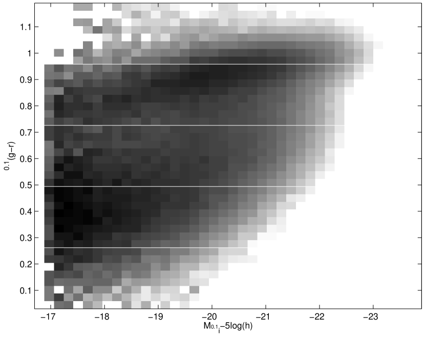
Figure 1: Two dimensional luminosity functions by colour and absolute magnitude taken from Blanton et al. (2003). White lines indicate the colours separating our different colour classes.

Figure 2: Schechter function fits to the luminosity functions of SDSS galaxies in our five different colour classes (see also Table 1).

Table 1: Definition of the different galaxy types according to their colour. Also the parameters of the Schechter function fits to the respective LF’s are given here.

	Colour    ${}^{0.1}(g-r)$			LF – Schechter fit
Type	mean	range		$\Phi[\mbox{Mpc/h}]^{-3}$	$\alpha$	${}_{{}^{0.1}i}M_{*}$
1	1.01	$0.96\dotfill 1.19$		$2.377\ 10^{-3}$	$-0.11$	$-20.96$
2	0.87	$0.73\dotfill 0.96$		$8.406\ 10^{-3}$	$-0.60$	$-20.61$
3	0.61	$0.49\dotfill 0.73$		$5.169\ 10^{-3}$	$-0.89$	$-20.49$
4	0.40	$0.26\dotfill 0.49$		$4.382\ 10^{-3}$	$-1.29$	$-19.84$
5	0.20	$0.03\dotfill 0.26$		$9.596\ 10^{-4}$	$-1.51$	$-19.11$

We use the fits of Fig. 2 to construct PLE models as described in Gardner (1998) – except for the slight complication that $z_{\mathrm{LF}}=0.1$. The five colour classes are identified with five SFH’s which reproduce their broad-band colours according to the stellar population synthesis models of Bruzual & Charlot (2003). For each galaxy type the spectrum and the LF can then be evolved backwards in time in order to predict the properties of the galaxy population at earlier redshifts.

The assignment of SFH to present-day colour is far from unique, so we construct a variety of possible models differing in their IMF, metallicity, formation redshift $z_{\mathrm{f}}$ (defined as the redshift when stars start to form) and e-folding timescale $\tau$ for an assumed exponentially declining SFR. We assume all colour classes to have the same $z_{\mathrm{f}}$, except for the bluest one, which often cannot be fit by any exponentially declining SFR. This is a particular problem for models with a steep IMF. In such cases we assume a SFH with constant SFR seen at a fixed age, implying no evolution with redshift. This is the standard fix for this problem, which is, in any case, irrelevant for the questions we study here.

We limit the range of allowed parameters in our PLE models by requiring consistency with the observed, apparently passive evolution of bright early-type galaxies in clusters. We require the $B$-band mass-to-light ratio of our reddest colour classes to evolve similarly to the measurements of van Dokkum & Stanford (2003). As the left three panels in Fig. 3 show, this mainly constrains the slope of the IMF, given that one has considerable freedom in the choice of the formation redshift $z_{\mathrm{f}}$. IMF’s with a power law exponent of $x=2.0$ (where the Salpeter exponent is $x=1.35$) are excluded, except possibly for the lowest formation redshifts. We nevertheless adopt this slope for Model 4 below in order to study its implications. We note that most recent work on IMF’s at high redshift have tended to argue for exponents significantly flatter than Salpeter (“top-heavy IMF’s”) in order to explain the high luminosities of sub-millimeter luminous galaxies and the apparently high aggregate metal yields of early generations of stars.

We also require the rest-frame $U$-$B$ colours of the reddest colour class to match those of bright ellipticals in two clusters, the Coma cluster at $z=0.023$ and MS 1054-03 at $z=0.87$ (Gavazzi et al., 1991; van Dokkum et al., 1999). This allows only a narrow range of metallicities for these bright early-types, namely approximately solar, as can be seen from the three right-hand panels in Fig. 3 which show the evolution in rest-frame colour for stellar populations of given metallicity formed with a Salpeter IMF in a single burst at a variety of redshifts. IMF variations have very little effect on this colour since it is dominated by main sequence turn-off stars (as explained by Bruzual & Charlot, 2003).

We present results for five representative models that are at least marginally consistent with all these constraints. Their parameters are summarised in Table 2 and were selected to cover the whole range of permitted values.

Figure 3: Left: Evolution of the mass-to-light ratio of cluster ellipticals in the $B$-band as given by van Dokkum & Stanford (2003). Small open symbols denote individual galaxies while big filled symbols stand for data averaged over a number of massive galaxies in a cluster. The model predictions are shown for different $z_{\mathrm{f}}$ and IMF slopes ranging from $x=1.35$ at the top to $x=2$ at the bottom. Right: Rest-frame $U$-$B$ evolution of model early-type galaxies compared to the rest-frame $U$-$B$ colours of cluster ellipticals at $z=0.87$ (MS 1054-03) and at $z=0.023$ (Coma). Model predictions are shown for different $z_{\mathrm{f}}$ and for three metallicities, $0.2Z_{\odot}$, $Z_{\odot}$ and $2.5Z_{\odot}$ from top to bottom.

Table 2: Definition of the different models. The given parameters are: slope of the IMF – x, formation redshift – $z_{\mathrm{form}}$, and exponential fall-off time of the SFR – $\tau$ (where $\infty$ means constant star formation).

Model	0	1	2	3	4
imf x	1.35	1.5	1.35	1.5	2.0
$z_{\mathrm{form}}$	15	15	3.5	3.5	3.5
$\tau_{1}$	1.5	2.0	1.5	1.5	1.5
$\tau_{2}$	3.0	3.0	2.5	2.5	3.0
$\tau_{3}$	6.0	10.0	5.0	7.0	30.0
$\tau_{4}$	$\infty$	${}^{*}\infty$	$\infty$	${}^{*}\infty$	${}^{*}\infty$
$\tau_{5}$	${}^{*}\infty$	${}^{*}\infty$	${}^{*}\infty$	${}^{*}\infty$	${}^{*}\infty$

The ^∗ denotes galaxy types without evolution.

2.2 The $K$-band LF as a consistency test

The LF’s used here were measured in the rest frame ${}^{0.1}i$-band. We can check the reliability of our stellar population models for the five colour classes by using them to predict the $K$-band ($2.2\,\mu\mathrm{m}$) luminosity function of local galaxies. This is of particular interest because near-IR light is a relatively good tracer of stellar mass, depending only weakly on dust content and SFH. We therefore compare the present-day $K$-band LF produced by our models to the observed function as given by Kochanek et al. (2001). As can be seen in Fig. 4, models and data agree reasonably well apart from a slight magnitude offset, perhaps $\sim 0.15\mbox{${}^{\mathrm{m}}$}$, at the bright end. This is likely due to the rather bright isophotal magnitudes used by Kochanek et al. in contrast to the surface-brightness independent Petrosian magnitudes of the SDSS survey. The difference is most pronounced for elliptical galaxies with de Vaucouleur-type surface brightness profiles. These dominate the bright end of the LF.

Figure 4: Comparison of our model $K$-band LF’s with the one that Kochanek et al. (2001) derived from 2MASS data. The slight offset at bright magnitudes can be accounted for by differing magnitude definitions in the SDSS and 2MASS surveys.

3 Comparison of $K$-band Selected Redshift Distributions

In this letter we compare to the same deep surveys as Somerville et al. (2004), namely GOODS CDF-S covering about $160\,\mathrm{arcmin}^{2}$ with photometric redshifts obtained by Mobasher et al. (2004) and K20 carried out in a smaller area of the same field covering $52\,\mathrm{arcmin}^{2}$ but providing spectroscopic redshifts rather than photometric ones (Cimatti et al., 2002a). The differential distribution of galaxies per $\mathrm{arcmin}^{2}$ and per unit redshift interval is shown in Fig. 5 for both datasets, binned to $\Delta z=0.15$ and with Poisson errorbars. Clearly there is some substructure in these distributions due to the relatively small fields surveyed. In particular at $z\sim 0.7$ there is a prominent peak in the K20 data. This feature is still visible in Fig. 6, the cumulative redshift distribution of galaxies. In a larger comoving volume such fluctuations should average out, which gives the smoother curves obtained for the somewhat larger GOODS survey.

Superposed on the observational data in Fig.’s 5 and 6 we show the differential and cumulative redshift distributions predicted by the various models specified in Table 2. In both figures directly predicted counts are given per $\mathrm{arcmin}^{2}$. In the inset of Fig. 6, however, we additionally show cumulative plots normalised to unity in order to show that the predicted redshift distributions differ in shape as well as in amplitude.

In order to quantify the obvious discrepancy between observations and models, Table 3 presents expected and measured counts integrated over various redshift ranges. The standard Salpeter model, model 0, overpredicts the observed counts beyond $z=1$ by a factor of almost 3, beyond $z=1.5$ by more than a factor of 5, and beyond $z=2$ by nearly an order of magnitude.

Figure 5: Differential redshift distributions for $K<20$ galaxies. The errors plotted on the observational data points are approximate Poisson errors. Our 5 PLE models are shown as contiuous curves as indicated in the figure.

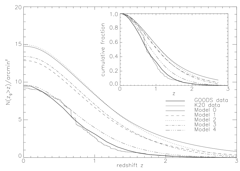
Figure 6: Cumulative redshift distributions corresponding to the differential distributions of Fig. 5. The inset shows the same distributions normalised to $1.0$ at $z=0$ rather than the absolute counts per $\mathrm{arcmin}^{2}$.

Table 3: Predicted and observed galaxy counts in the range $1<z<3$.

	Counts [$\mbox{arcmin}^{-2}$]
Model	$z\geq 1$	$z\geq 1.5$	$z\geq 2$	$z\geq 2.5$	$z\geq 3$
0	$8.36$	$4.76$	$2.65$	$1.48$	$0.80$
1	$6.66$	$3.46$	$1.70$	$0.81$	$0.35$
2	$8.47$	$4.62$	$2.22$	$0.88$	$0.21$
3	$7.05$	$3.62$	$1.62$	$0.58$	$0.11$
4	$3.96$	$1.56$	$0.50$	$0.12$	$0.01$
K20	$2.63$	$0.73$	$0.17$	$0.06$	$0.00$
GOODS	$3.04$	$0.93$	$0.29$	$0.04$	$0.00$

4 Discussion and Conclusions

The problem we study in this letter is whether the available observational data are consistent with present day luminous galaxies being already assembled with the bulk of their stars formed at high redshift. If so, it should be possible to find a set of parameters such that traditional PLE models can simultaneously reproduce: (i) the present-day luminosity and colour distributions of massive galaxies; (ii) the passive evolution in colour and M/L ratio observed for massive early-type galaxies in clusters; and (iii) the observed galaxy counts as a function of redshift in deep surveys. Near-IR limited surveys are best suited for this purpose since the observed magnitudes are then a fair indicator of stellar mass and are only weakly affected by dust. We therefore chose $K$-band data from the K20 and GOODS CDF-S surveys for comparison with our models.

Out to redshift $z\sim 1$ our model predictions are very similar to each other and also fit the data reasonably, given their error bars. At higher redshifts all models predict too many galaxies. Only Model 4, with $x=2$, comes close to the data. Obviously the IMF assumed has the largest impact on the predicted number of galaxies at high redshift; the second and third best models are the two with $x=1.5$. Changing the formation redshift only mildly influences the shape of the distributions at $z<2.5$. The more conventional standard Model 0, using a Salpeter IMF, and its low $z_{\mathrm{f}}$ pendant, Model 1, produce the predictions most inconsistent with the data. This may be understood by recalling that the light of old stellar populations is dominated by stars with masses near the main sequence turn-off. For younger populations this turn-off is at higher masses. Hence a shallower IMF, corresponding to more turn-off stars in younger populations, implies brighter galaxies at early times, and so more high redshift galaxies above any apparent magnitude limit. The $B$-band M/L ratio evolution of the brightest and reddest galaxies is an important constraint on our models because it is also sensitive to the IMF for the same reasons. As already noted in Section 2.1 models with $x=2$ are inconsistent with observation, except possibly for very low formation redshifts. Additionally, for $x=2$ our models cannot fit the observed present-day colours of the bluest galaxy classes for constant SFR and $z_{\mathrm{f}}\geq 3.5$. For the galaxies to be blue enough they would have to be much younger. Missing bright blue stars at the high mass end of the IMF again account for the effect. Finally, since most models for the light output and metal production of high redshift galaxies require IMF’s with substantially more high mass stars than Salpeter (e.g. Nagashima et al., 2004), an IMF as steep as $x=2$ appears very unlikely as an explanation of the apparent lack of high redshift massive galaxies.

Our Model 0 is very similar to the PLE model used by Somerville et al. (2004) but whereas we find it to be badly inconsistent with the data, they conclude that any problem is marginal. There are two reasons for this discrepancy. Looking at their Figure 1 there is clearly a problem in going from their differential redshift distribution, which is very similar to our own, to the cumulative distribution, which predicts substantially fewer high redshift galaxies than does ours. In addition, they compare the cumulative distribution to the data after normalising both to unity (as in the inset to Fig. 6) which then misses the fact that the total predicted galaxy count at K$<20$ is substantially larger than observed.

All of our models with $x\leq 1.5$ overpredict the counts at redshifts $z>1$ by a large factor as can be seen in Table 3. In the interval $1<z<2$ these models all predict more than twice the number of galaxies observed and in the interval $2<z<3$ they are off by factors between 4 and 11. Could cosmic variance or dust account for this? The clustering of galaxies has the greatest effect at low redshift, where the observed volume is comparatively small and clear evidence of large fluctuations is seen in Fig. 5 at $z=0.7$ in the K20 data. However in this range the models still agree quite well with the data, only at higher redshifts do they deviate. Also the model predictions are obviously systematically too high at all $z$ which is not what one would expect if the effect was due to cosmic variance. Finally, models and data also disagree in the normalised version of the diagram (inset in Fig. 6).

Extinction by dust, on the other hand, might indeed be important. As a simple model to assess how much dust is required to bring our PLE models into agreement with the data, consider placing a foreground screen in front of all galaxies at $z=1.5$, thereby translating their apparent luminosity function fainter by some fixed amount. We find that to lower the count for Model 0 in Fig. 5 by the factor of $2.1$ needed to bring it into agreement with the GOODS data at this redshift requires $0.7$ magnitudes of extinction at observed K (i.e. at rest-frame $z$). Carrying out a similar calculation at $z=2$ we find that $1.0$ magnitudes of extinction is again required at observed K (now rest-frame $r$) to reduce the abundance of galaxies per unit redshift by the required factor of $5.1$. For comparison Kauffmann et al. (2003) analysed dust attenuation in a sample of 122808 low redshift galaxies drawn from the SDSS, finding a typical (median) attenuation of 0.2 – 0.3 magnitudes in the $z$-band for massive galaxies. We thus need much more dust in high redshift massive galaxies than is seen in local galaxies to reconcile our PLE models with the data. Note that this dust must be present without an accompanying population of younger stars, which would raise the intrinsic luminosity of the stellar population of the galaxy. In the nearby universe such populations are almost always present in dusty galaxies and the effects of the young stars cancel almost exactly those of the dust, resulting in a colour–apparent M/L relation which depends very weakly on dust content (Bell & de Jong, 2001; Kauffmann et al., 2003). If high redshift galaxies behave similarly, then dust will not help reconcile our PLE models with the data.

Our main conclusion is that traditional PLE models cannot reconcile the relatively small number of high redshift galaxies found in deep K-selected redshift surveys with the abundance of massive galaxies seen in the local Universe. The counterparts of nearby luminous red galaxies just do not seem to be present in sufficient numbers at redshifts of 1.5 to 2. The areas of the deep surveys are quite small, so there may still be significant uncertainties in this statement as a result of cosmic variance. Substantial amounts of dust might also cause many distant massive galaxies to be missed, but only if dust attenuation is not compensated by emission from young stars in the way observed in low redshift galaxies. If these two possibilities are insufficient to explain the discrepancy, then one will be forced to conclude that most nearby massive galaxies were assembled at $z<1.5$, presumably by mergers of pre-existing stellar systems, since their stars appear to be old.

References

- Bell & de Jong (2001) Bell, E. F. & de Jong, R. S. 2001, ApJ, 550, 212
- Blanton et al. (2003) Blanton, M. R., Hogg, D. W., Bahcall, N. A., et al. 2003, ApJ, 594, 186
- Bruzual & Charlot (2003) Bruzual, G. & Charlot, S. 2003, MNRAS, 344, 1000
- Cimatti et al. (2002a) Cimatti, A., Mignoli, M., Daddi, E., et al. 2002a, AAp, 392, 395
- Cimatti et al. (2002b) Cimatti, A., Pozzetti, L., Mignoli, M., et al. 2002b, AAp, 391, L1
- Firth et al. (2002) Firth, A. E., Somerville, R. S., McMahon, R. G., et al. 2002, MNRAS, 332, 617
- Fontana et al. (1999) Fontana, A., Menci, N., D’Odorico, S., et al. 1999, MNRAS, 310, L27
- Gardner (1998) Gardner, J. P. 1998, PASP, 110, 291
- Gavazzi et al. (1991) Gavazzi, G., Boselli, A., & Kennicutt, R. 1991, AJ, 101, 1207
- Kashikawa et al. (2003) Kashikawa, N., Takata, T., Ohyama, Y., et al. 2003, AJ, 125, 53