Searching for Planetary Transits in Galactic Open Clusters: EXPLORE O/C

Abstract

Open clusters potentially provide an ideal environment for the search for transiting extrasolar planets since they feature a relatively large number of stars of the same known age and metallicity at the same distance. With this motivation, over a dozen open clusters are now being monitored by four different groups. We review the motivations and challenges for open cluster transit surveys for short-period giant planets. Our photometric monitoring survey (EXPLORE/OC) of Galactic southern open clusters was designed with the goals of maximizing the chance of finding and characterizing planets, and of providing for a statistically valuable astrophysical result in the case of no detections. We use the EXPLORE/OC data from two open clusters NGC 2660 and NGC 6208 to illustrate some of the largely unrecognized issues facing open cluster surveys including severe contamination by Galactic field stars ($>$ 80%) and relatively low number of cluster members for which high precision photometry can be obtained. We discuss how a careful selection of open cluster targets under a wide range of criteria such as cluster richness, observability, distance, and age can meet the challenges, maximizing chances to detect planet transits. In addition, we present the EXPLORE/OC observing strategy to optimize planet detection which includes high-cadence observing and continuously observing individual clusters rather than alternating between targets.

1 Introduction

The EXPLORE Project (Mallén-Ornelas et al., 2003; Yee et al., 2003) is one of currently about 20 ongoing surveys with the aim to detect transiting close-in extrasolar giant planets (CEGPs; also referred to as ‘51-Peg type’ or ‘hot Jupiters’, i.e., planets with radius of order Jupiter-radius, orbital period of one to a few days, and transit durations of a few hours) around Galactic main-sequence stars. Transit studies explore a different parameter space in the search for extrasolar planets from the very successful radial-velocity or “wobble” method. This method based on detecting planets via the radial motions of their parent star caused by the star’s motion about the common center of mass (see for example table 3 in Butler et al., 2002). Fainter (and thus more) stars can be monitored photometrically than spectroscopically. Thus, more distant environments can be probed for the existence of extrasolar planets.

All transiting planets have a measured radius, based on transit depth and stellar radius. Knowledge of the planet’s radius and mass plays an important role in modeling internal structure of planets and hence the formation, evolution, and migration of planetary systems (see for example Burrows et al., 2000; Guillot & Showman, 2002; Baraffe et al., 2003, and references therein).

Transiting planets are currently the only planets whose physical characteristics can be measured. In addition to mass and radius, several parameters can be constrained from follow-up measurements. For example, the fact that a transiting planet will be superimposed on its parent star can be used to determine constituents of the planet’s atmosphere by means of transmission spectroscopy (Charbonneau et al., 2002; Vidal-Madjar et al., 2003), or put constraints on the existence of planetary moons or rings (e.g., Brown et al., 2001). In addition, the secondary eclipse can provide information about the planetary temperature or its emission spectrum (Richardson et al., 2003a, b).

At the time of writing, six transiting planets are known. HD209458b (Charbonneau et al., 2000; Henry et al., 2000; Brown et al., 2001) was discovered by radial-velocity measurements (Henry et al., 2000; Mazeh et al., 2000) and the transits were discovered by photometric follow-up. OGLE-TR-56 (Udalski et al., 2002a, b; Konacki et al., 2003a) was the first planet discovered by the transit method, and the first of currently four planets based on photometry of the OGLE-III survey (Udalski et al., 2002a, b, 2003): OGLE-TR-113 (Bouchy et al., 2004; Konacki et al., 2004), OGLE-TR-132 (Bouchy et al., 2004), and OGLE-TR-111 (Pont et al., 2004). Very recently, Alonso et al. (2004) found a further transiting planet, TrES-1, using telescopes with 10cm apertures. Over 20 transit searches are currently ongoing to find more planets.

As part of the EXPLORE Project, we have recently begun a survey – EXPLORE/OC – of southern open clusters (OCs) with the aim of detecting planetary transits around cluster member stars. During the course of $\sim$3 years, we hope to conduct searches of up to 10 OCs using the Las Campanas Observatory (LCO) 1m Swope Telescope. To date we have monitored five OCs (see §6).

In addition to EXPLORE/OC, at the time of writing there are currently three OC planet-transit surveys underway:

• The Planets In Stellar Clusters Extensive Search (PISCES) reported the discovery of 47 and 57 low-amplitude variables in the open clusters NGC 6791 (Mochejska et al., 2002) and NGC 2158 (Mochejska et al., 2004), respectively.

• The University of St. Andrews Planet Search (UStAPS) has monitored the OCs NGC 6819 (Street et al., 2002) and NGC 7789 (Bramich et al., 2003) and published data on variable stars in NGC 6819 (Street et al., 2003).

• The Survey For Transiting Extrasolar Planets In Stellar Systems (STEPSS), described in Burke et al. (2003) and Gaudi et al. (2002). They have analyzed monitoring data of the OC NGC 1245 (Burke et al., in preparation) and determined its fundamental parameters (Burke et al., 2004). Analysis of their data on NGC 2099 and M67 is currently ongoing.

The OC NGC 6791 was furthermore monitored for planetary transits by Bruntt et al. (2003). As all these surveyed OCs are located the northern hemisphere, EXPLORE/OC is currently the only OC survey operating in the south where most of the Galactic OCs are located.

With the growing number of open star cluster surveys this publication describes incentives, difficulties, and strategies for open cluster planet transit surveys, thereby including a discussion on transit surveys in general. We use data from the first two targets (NGC 2660 and NGC 6208) from our program to illustrate the major issues for OC transit surveys.

The concept and advantages of monitoring OCs for the existence of transiting planets were originally described in Janes (1996). Written before the hot Jupiter planets were discovered, Janes (1996) focused on 12-year period orbits and long-term photometric precision required to determine or put useful limits on the Jupiter-like planet frequency. This paper is intended to be a modern version of Janes (1996) based on the existence of short-period planets and practical experience we have gained from both the EXPLORE and the EXPLORE/OC planet transit surveys. Section 2 motivates OC transit surveys. Section 3 addresses the challenges facing transit surveys in general, and §4 addresses challenges specifically facing OC transit surveys. Section 5 focuses on strategies to select OCs which are most suited for transit surveys and which minimize challenges described in the previous sections. The EXPLORE/OC strategies concerning target selection, observing methods, photometric data reduction, and spectroscopic follow-up observations are described in §6, §7, and §8, respectively. These Sections contain relevant preliminary results on EXPLORE/OC’s first two observed clusters NGC 2660 and NGC 6208. We summarize and conclude in §9.

2 Motivation for Open Cluster Planet Transit Searches

Open clusters present themselves as “laboratories” within which the effects of age, environment, and especially metallicity on planet frequency may be examined. Evidence that planet formation and migration are correlated with metallicity comes from radial velocity planet searches (Fischer & Valenti, 2003). The fact that no planetary transits were discovered in the monitoring study of 47 Tuc by Gilliland et al. (2000) may be due to its low metallicity, or alternatively due to the high-density environment in a system such as a globular cluster (or due to both effects). The less-crowded OCs of the Milky Way offer a range of metallicities and may thus be further used to disentangle the effects of metallicity versus high-density environment upon planet frequency.

Monitoring OCs for the existence of planetary transits offers the following incentives (see also Janes, 1996; Charbonneau, 2003; Lee et al., 2004; von Braun et al., 2004):

1. Metallicity, age, distance, and foreground reddening are either known or may be determined for cluster members (more easily and accurately than for random field stars; see §5 and, e.g., Burke et al., 2004). Thus, planets detected around open cluster stars will immediately represent data points for any statistic correlating planet frequency with age, stellar environment, or metallicity of the parent star.

2. The planet-formation and planet-migration processes, and hence planet frequencies, may differ between the OC, globular cluster, and Galactic field populations. Planet transit searches in OCs, together with many ongoing transit field searches and GC surveys (e.g., the ground-based work on 47 Tuc by Weldrake et al., 2003, 2004), enable comparison between these different environments.

3. Specific masses and radii for cluster stars may be targeted (within certain limits of other survey design choices, see §7.2) in the planet-search by the choice of cluster distance and by adjusting exposure times for the target.

3 Main Challenges for Transit Surveys

Open cluster planet transit surveys are a subset of planet transit surveys and therefore have some important challenges in common. Articulating these challenges is crucial in light of the fact that over 20 planet transit surveys have been operating for a few years (Horne, 2003), with only six known transiting planets of which five were discovered by transits.

The most basic goals of any transit survey are to (1) detect planets and provide their characteristics, and (2) to provide (even in the case of zero detections) statistics concerning planet frequencies as a function of the astrophysical properties of the surveyed environment. Although the most important considerations for designing a successful transit survey were presented in Mallén-Ornelas et al. (2003, M03 hereafter) for the EXPLORE Project, we summarize and provide updates to the three key issues: number of stars, detection probability, and blending. For OC surveys, these issues (with the exception of blending) can be optimized or overcome by a careful survey strategy, particularly by the selection of the target OC (see §5 through 7).

3.1 Maximizing Number of Stars with High Photometric Precision

Any survey’s goal should be to maximize the number of stars for which it is possible to detect a transiting planet. We discuss the three most important aspects below: the astrophysical frequency of detectable transiting planets, the probability with which existing planetary transits are observed, and the number of stars for which the relative photometric precision is sufficiently high.

The frequency of detectable transiting planets is calculated by considering the astrophysical factors: frequency of CEGPs around the surveyed stars; likelihood of the geometrical alignment between star and planet necessary to detect transits; and binary fraction. We assume a planet frequency around isolated stars of 0.7% for planets with semi-major axis $a\sim 0.05$ (Marcy et al., 2004; Naef et al., 2004). Of those CEGP systems, approximately 10–20% (probability $\sim R_{*}/a$) would, by chance, have a favorable orientation such that a transit is visible from Earth. We assume that planets can only be detected around single stars and conservatively adopt a binary fraction of 50%; although there are known planets orbiting binary stars and multiple star systems (Zucker & Mazeh, 2002; Eggenberger et al., 2004), their detection by transits would be difficult due to a reduced photometric signature in the presence of the additional star. Combining the above estimates, we arrive at the at the value of 1 star in 3000 ($a\sim 0.05$ AU) having a hot Jupiter planetary transit around a main sequence star.

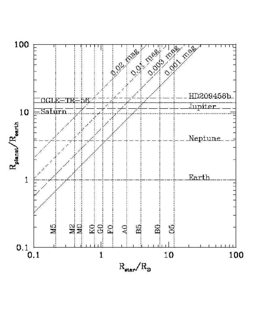
Figure 1: Depth of transit signal for transiting planets with different radii as a function of MK spectral type and corresponding stellar sizes (from Cox, 2000) based on geometric arguments only. The diagonal lines indicate the amplitude of the transit signal in the light curve of a given planet–star combination. For instance, a Jupiter-sized planet would cause a 0.01 mag dip in the light curve of a G0 star, but only a 0.003 mag dip in the light curve of an A0 star.

The probability of detecting an existing transiting hot Jupiter (1/3000) applies only to stars for which it is possible to detect a planetary transit given the observational setup of the survey. This number of “suitable” stars is frequently equated to the number of stars with high enough relative photometric precision to detect the transiting planet (see Fig. 1). Planet transit surveys in general reach photometric precision sufficiently high to detect Jupiter-sized transiting planets around main sequence stars (see Fig. 1) for up to 40% of stars in their survey, depending on crowdedness and other factors. For example, the EXPLORE search reached relative photometric precision better than 1% on 37,000 stars from $14.5\leq I\leq 18.2$ out of 350,000 stars down to $I=21$ (M03); OGLE-III reached better than 1.5% relative photometric precision on 52,000 stars out of a total of 5 million monitored stars (Udalski et al., 2002b); the Sleuth survey (O’Donovan et al., 2004), reaches better than 1.5% relative photometry over the entire dataset on the brightest 4000 stars out of 10,000 in their 6$\times$6 degree² field, using an automated 10 cm telescope with a 6 degree square field of view.

The real number of stars suitable for planet transit detection, however, is not equivalent to the number of stars with 1% relative photometry. One may see from Fig. 1, for instance, that a Jupiter-sized planet would cause a 2% eclipse around a parent M0-star. Furthermore, Pepper & Gaudi (in preparation) find that, if a planet with given properties around a cluster member star on the main sequence produces a detectable transit signature, a planet with identical properties orbiting any other main-sequence cluster member will produce a detection of approximately the same signal-to-noise-ratio (SNR) unless the sky flux within a seeing disk exceeds the flux of the star. Since most transit surveys aim to find planets of approximately Jupiter-size around stars whose radii are close to, or less than, a solar radius, the number of stars with 1% relative photometric precision can therefore be regarded as a lower limit to the number of stars suitable for transit detection. For the rest of this publication, we thus use this number as a proxy for the number of stars around which we (or other transit surveys) can detect planets.

3.2 Probability to Detect an Existing Transit

The actual observed hot-Jupiter transit frequency will be lower than 1/3000 due to the probability with which an existing transit would be observed two or more times during an observing run. This probability, which we call $P_{vis}$, is equivalent to the window function of the observations. Although the probability function has been described in detail before (Borucki & Summers, 1984; Gaudi, 2000, and M03), we extend the discussion to include the recently discovered class of 1-day period planets, as well as considering different metrics for probability to detect an existing planet. In all of our $P_{vis}$ simulations we assume the simplified case of a solar mass, solar radius star with the planet crossing the star center, thus focusing on stars we are most interested in. The transit duration is then related to the planet’s period by $t_{\rm duration}=PR_{\odot}/\pi a$ (typically a few hours for a period of a few days).

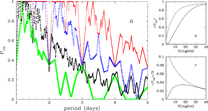
Figure 2: Probability $P_{vis}$ of detecting existing transiting planets with different orbital periods. $P_{vis}$ is calculated with the requirement that two full transits must be observed. Panel a: $P_{vis}$ of detecting 2 transits of an existing transiting planet with a period between 1 and 5 days after 21 (top curve), 14 (second curve from the top) and 7 (bottom curve) consecutive, uninterrupted nights of observing (10.8 hours per night). The difficulty of detecting some phases is shown by the dips in the curves (e.g., orbital periods of an integer number of days may always feature their transits during the day and are therefore statistically harder to detect). All phases are averaged over for each period. The second curve from the bottom shows the real $P_{vis}$ for our monitoring study of NGC 2660 (19 nights of 7-8 hours per night, with interruptions due to weather and telescope scheduling; see Fig. 7). Panel b: The mean $P_{vis}$ (averaged over 1 day $<P<$ 5 days) as a function of number of consecutive nights in an observing run. The solid line is for the requirement to detect two transits and the dashed line for one transit. This figure indicates how much the likelihood of finding existing transits grows with an increasing number of nights of observing. Panel c: Run efficiency (defined as $<P_{vis}>$ divided by the number of observing nights) as a function of run length. For the two-transit requirement (solid line) and, an observing run of 18 nights is most efficient. For the single transit requirement, the efficiency decreases monotonically with the number of nights since additional nights have progressively lower probabilities of detecting ”new” transits.

In panel a of Figure 2 we show the $P_{vis}$ for detecting existing transiting planets with different orbital periods under the requirement that two or more full transits must be observed. We consider different runs (7, 14, 21 nights) of consecutive nights with 10.8 hours of uninterrupted observing each night with 5-min time-sampling. This is equivalent to approximately 125 observations of a given cluster per night. The $P_{vis}$ for 1- to 2-day period planets is basically complete for the 14- and 21-night runs, while the $P_{vis}$ is markedly lower for a 14-night run compared to a 21-night run for planets with periods between 2 and 4 days.

We now turn to $P_{vis}$ for a transit detection strategy where it is not necessary to detect a transit in its entirety during a single observing night. Instead, the strategy requires a transit to be detected in phased data (from at least two individual transit events). Such a $P_{vis}$ (which we call $Pvis_{phased}$) is relevant for transit detections based on period-folding transit-searching algorithms (for instance with data covering partial nights or a strategy of alternating targets throughout the course of a night). With a period-folding algorithm, each individual transit need not be fully sampled. In order to quantify $Pvis_{phased}$, we specify that the phased transit must be sampled by at least $N$ points. Since a typical duty cycle of a transit is on the order of a few percent, we choose $N$ = 20, 40, or 60 to represent light curves with a total of a few hundred to a thousand data points (the phased OGLE planets’ light curves typically have a few tens of data points obtained during transit). $Pvis_{phased}$ is then calculated to be likelihood (as a function of period) that at least $N$ in-transit points are accumulated for observing runs of different lengths and different observing cadences.

Note that in reality a detection of a planet transit depends on the number of photons observed during the transiting phase. This number of photons is contained in the combination of the SNR per individual data point and the number of data points (during any transit). A back-of-the-envelope calculation would give a transit SNR for a $\Delta m\sim$ 2%-depth transit with $M=20$ data points and a relative photometry precision of rms $\sim$1%:

$$SNR\simeq\sqrt{M}\times\frac{\Delta m}{{\rm rms}}=\sqrt{20}\times\frac{0.02}{0.01}\sim 9.$$ (1)

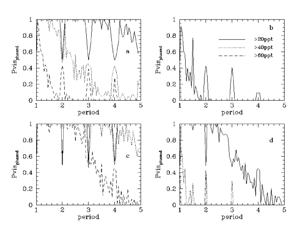
Figure 3: $Pvis_{phased}$ as a function of period (in days) for detecting planetary transits in phased data. $Pvis_{phased}$ is calculated to be likelihood that at least $N=20$ (solid line), 40 (dotted line), or 60 (dashed line) in-transit points are are accumulated for observing runs of different lengths and different observing cadences. The number of points per transit required for a detection is dependent on both SNR and exposure time. Panels a and b compare $Pvis_{phased}$ for a 21-night (10.8h) observing run with a cadence of 5 minutes (panel a) and 15 minutes (panel b). Panels c (5-minute cadence) and d (15-minute cadence) illustrate the same for a observing run of 40 nights. See text (§3.2) for discussion.

For comparison with the two-full-transit $P_{vis}$, we show in Fig. 3 $Pvis_{phased}$ for $N=20,40,60$ by a solid, dotted, and dashed line, respectively. The four panels represent different observing strategies:

• Panel a shows $Pvis_{phased}$ for 21 nights (10.8h) with 5-minute time-sampling, resulting in a light curve with around 2700 data points. If the data SNR is high enough for 20 data points during transit to constitute a detection, then $Pvis_{phased}$ is high for all transit periods between one and five days. If, in contrast, the data SNR is lower, and 40 or 60 points per transit are required for detection, then $Pvis_{phased}$ is low for $P>2$ days.

• Alternatively, one could imagine a strategy of alternating between cluster fields (to increase the number of monitored stars), in which case the observing cadence is reduced. Panel b shows $Pvis_{phased}$ when observing for 21 nights with a 15-minute cadence ($\sim$ 900 measurements in the light curve). The probability to detect transits with $N=20$ is very low for $P>2$ days, and it is zero for $N=40$ or 60.

• Panel c shows $Pvis_{phased}$ for 40 nights of continuous observing (10.8h) with an observing cadence of 5 minutes ($\sim$ 5200 data points). For $N=20$ and $N=40$, $Pvis_{phased}$ is close to complete for all shown periods.

• Panel d shows $Pvis_{phased}$ for 40 nights of observing with a 15-minute cadence (again simulating a strategy of alternating between cluster fields; $\sim$ 1700 data points). $Pvis_{phased}$ is very low for $N>20$, indicating that, in order to be able to observe with a 15-cadence, many more than 40 nights are needed if more than 20 data points are required for a transit detection.

We conclude that the ability to particularly detect longer-period ($P>$ 2 days) planets depends on observing strategy. For the rest of this paper we adopt the $P_{vis}$ criterion of seeing two full transits which is a good strategy for a limited number ($\sim 20$) of observing nights.

3.3 Blending and False Positives

Blending in a planet transit light curve due to the presence of an additional star is a serious challenge inherent in planet transit surveys, one that has only recently been gaining recognition. If the light of multiple stars are interpreted as being due to one individual star, then the relative depth of any eclipse will be decreased. This “light pollution” may either cause (1) an eclipsing binary systems to mimic a more shallow transiting planet signal, or (2) a true planet’s transit signal’s depth to be decreased to a fraction of its already very small amplitude, rendering it harder or even impossible to detect.

Blending can be caused either by optical projection in crowded fields, or by physically associated stellar systems. The crowdedness can be considered in the choice of target and observational setup. Blending in spatially unresolved, physically associated systems generally consists of a wide binary of which one component hosts an additional close-by stellar companion or a transiting planet. The component without the close-by stellar or planetary companion would produce the polluting light. Although we have accounted for binary stars in our probability estimate (§3.1), the contribution due to this kind of “false positive” may be larger due to the unknown wide-binary component distances.

Recently the effect of blending on the probability of detecting planets has been addressed by several authors (e.g., M03; Brown, 2003; O’Donovan et al., 2004; Konacki et al., 2003b) in the context of causing false positives. Several solutions have been proposed to avoid false positive transit candidates that are actually blended star light curves. Seager & Mallén-Ornelas (2003) show that one may eliminate some false positives due to blending with photometric data alone if the light curve is of sufficient relative photometric precision and the observing cadence is high enough to clearly resolve the individual temporal components of the transit. Using spectroscopic data, other solutions include a careful modeling of the additional star properties to detect a second cross correlation peak caused by a physically associated star (M03; Konacki et al., 2003b; Kotredes et al., 2003; Torres et al., 2004b). Finally, estimates for blending (associated either with chance alignment of foreground or background stars, or physical triplets) effects on the probability of detecting existing transits can be quantified for individual surveys, as done by Brown (2003) for shallow wide-field transit surveys.

4 Main Challenges for Open Cluster Transit Surveys

The difficulties and challenges involved in searching for planetary transits specifically in OCs are: the fixed and somewhat low number of stars in an open cluster, determining OC cluster membership in the presence of significant contamination, and differential reddening along the cluster field and along the line of sight. We outline these aspects individually below.

1. The Number of Monitored Stars The number of monitored stars is typically lower than in rich Galactic fields (in part due to the smaller field size of the used detectors), reducing the statistical chance of detecting planets. Open clusters can have up to $\sim$ 10,000 member stars (Friel, 1995), depending on the magnitude range taken into consideration. Only a subset of these stars, perhaps 10–20%, however, will be observed with sufficient relative photometric precision to detect transits (cf. §3.1). The number of these stars in rich OCs is comparable to the number in wide-field, shallow transit surveys, e.g., Sleuth: $\sim$4000 stars in 6$\times$6 square degrees of $9<R<16$ (O’Donovan et al., 2004); WASPO: $<$ 3000 stars in 9$\times$9 square degrees of broadband magnitude between 8 to 14 (Kane et al., 2004). The richest deep galactic fields surveyed have many more stars with high relative photometric precision (§3.1).

2. Cluster Contamination Determining cluster membership of stars in the OC fields without spectroscopic data or proper motion information is difficult due to significant contamination by Galactic field stars, since the clusters are typically concentrated toward the Galactic disk. For example, Street et al. (2003) estimate the contamination of Galactic field stars in their study of NGC 6819 to be around 94%. A study by Nilakshi et al. (2002) calculated the average contamination in the fields of 38 rich OCs to be 35% in the inner regions and 80% in the “coronae” of the clusters. Furthermore, if the target is located such that the line of sight includes a long path through the Galaxy (e.g., low Galactic latitude and longitude towards the Galactic bulge), background giants may start polluting the sample of stars with apparent magnitudes monitored with high relative photometric precision (see for example the discussion in Street et al., 2003). Getting a handle on the issue of contamination is vital for OC surveys since any statistical statements about the result will need to be based on estimates of surveyed cluster members.

3. Differential Reddening Differential reddening across the cluster field and along the line of sight can make isochrone fitting (and subsequent determination of age, distance, and metallicity) difficult. Ranges of $\Delta E_{B-V}\sim 0.2$ or higher across fields-of-view of 10–20 arcmin on the side are not uncommon (see for example the studies by Munari & Carraro, 1996; Raboud et al., 1997; Rosvick & Balam, 2002; Carraro & Munari, 2004; Villanova et al., 2004; Prisinzano et al., 2004). For an $R_{V}=3.1$ reddening-law, a differential $\Delta E_{B-V}\sim 0.2$ corresponds to a differential $\Delta V\sim 0.6$ and $\Delta I\sim 0.3$ (Cardelli et al., 1989). The calculated effective temperature of a solar-metallicity main-sequence star with $V-I\sim 0.8$ would vary by about 500 K for a differential reddening effect of $\Delta E_{B-V}\sim 0.2$ (Houdashelt et al., 2000). It should, however, also be noted that some OCs do not seem to suffer from differential reddening, such as NGC 1245 as examined in Burke et al. (2004) and NGC 2660 in our preliminary analysis of its CMD.

5 Open Cluster Selection

Open cluster target selection can help overcome or reduce some of the main challenges of OC planet transit surveys described in §3 and §4. More specifically, careful cluster selection can help maximize the number of stars, maximize the probability of detecting existing transits, and reduce line-of-sight and differential reddening. Most importantly, cluster selection allows for targeting specific spectral type for a given telescope and observing cadence.

The biggest challenge in the selection of target clusters is the paucity of data about many OCs. The physical parameters of the cluster, such as distance, foreground reddening, age, and metallicity are frequently either not determined, or there exist large uncertainties in the published values. For example, out of approximately 1100 associations of stars designated as OCs, many only have identified coordinates, approximately half have an established distance, and about 30% have an assigned metallicity (WEBDA database Mermilliod, 1996). Additional difficulties arise when independent studies arrive at different values for any of the parameters. For instance, the metallicity of NGC 2660 was determined to be as low as -1.05, and as high as +0.2 (see discussion in the introduction of Sandrelli et al., 1999). The very important criterion of richness tends to be even less explored than the other physical parameters, probably due to the significant contamination from field stars that these OCs tend to suffer.

In spite of the lack of OC data, a very useful place to start is the WEBDA database (Mermilliod, 1996). From the long list of potential OC monitoring targets, one can then start eliminating cluster candidates by applying the criteria we describe below.

5.1 Cluster Richness and Observability

Apart of its observability for a given observing run, the most important selection criterion for a cluster is its richness, simply to increase the statistical chance of detecting planets. The richness of the cluster field can be estimated by looking at sky-survey plots of the appropriate region. Estimating the richness of the cluster itself is a much more difficult process since field star contamination is usually significant due to the typically low Galactic latitude of the Pop. I OCs (see below and Bramich et al., 2003; Street et al., 2003; Burke et al., 2004). One may use published cluster richness classifications, such as in Cox (2000), taken from Janes & Adler (1982). The WEBDA database also contains information for clusters in the 1987 Lynga catalog (online data published in Lynga, 1995). The data published there, however, only present lower estimates for richness classes. The depths of the studies from which the richness classes were derived may differ significantly from one study to the next. Thus, these classes are rough estimates only, and the best way to judge the richness of a cluster field is to rely on one’s own test data obtained with the same setup as the one used for the monitoring study (see §7.5).

5.2 Cluster Distance

The distance to the target cluster is an important criterion for cluster selection for four reasons: (1) to ensure the cluster is sufficiently distant to fit into the field of view, (2) to allow RV follow-up of potential candidates, (3) to target the desired range of spectral types for given observing conditions, and (4) to minimize reddening.

Since all stars in an OC are at approximately the same distance, one may, with appropriate adjustment of the exposure time for given telescope parameters, cluster distance, and foreground reddening, target certain spectral types of stars for high-precision photometry. We are interested in G0 or later spectral type/smaller stars, since early-type stars have larger radii which would make transit detections more challenging. The transit depth in the light curve is, for small $\Delta m$, simply given by

$$\Delta m\simeq\frac{\Delta F}{F_{0}}=\left(\frac{R_{planet}}{R_{star}}\right)^{2},$$ (2)

where $\Delta m$ and $\Delta F$ are the changes in magnitude and flux, respectively, and $F_{0}$ is the out-of-transit flux of the parent star (see Fig. 1). In addition to featuring larger radii, early spectral types are fast rotators which exhibit broad spectral lines, making mass-determination of planetary companions more difficult.

Foreground reddening, increasing with cluster distance, usually represents a proxy for the amount of differential reddening across the field of view as well as along the line of sight (Schlegel et al., 1998). Differential reddening will cause the main sequence of the cluster to appear broadened (e.g., von Braun & Mateo, 2001). This, in turn, will cause large errors in the determination of cluster parameters such as age, metallicity, etc, by means of isochrone fitting. Furthermore, a broad main sequence will make any attempts to estimate contamination (based on isochrone fitting; see for example Mighell et al., 1998; von Hippel et al., 2002) more challenging.

5.3 Cluster Age

The consideration of cluster age in the OC selection is not as crucial as richness, observability, and distance. However, choosing both younger and older OCs may impose different challenges with respect to the transit-finding process.

Stellar surface activity, which would introduce noise into the light curve of a given star, decreases with age. As they age, stars lose angular momentum and thus magnetic activity on their surfaces (see for example Donahue, 1998; Wright, 2004, and references therein). The photometric variability for a sample of Hyades OC stars was found to be on the order 0.5–1% (Paulson et al., 2004) with periods in the 8–10 day range (the Hyades cluster has an age of $\sim$650 Myr; see Perryman et al., 1998; Lebreton et al., 2001). While these photometric variations do not necessarily represent a source of contamination in the sense of creating false positives, they nevertheless will introduce noise into the stellar light curves and thus render existing transits more difficult to detect.

Stellar surface activity is potentially an issue not just for host star photometric variability, but more so for radial velocity follow-up. Paulson et al. (2004) found that radial velocity rms due to rotational modulation of stellar surface features can be as high as 50 m/s and is on average 16 m/s for the same sample of Hyades stars. Further such correlation between radial velocity rms and photometric variability was found by Queloz et al. (2001) who observed a $v_{r}$ amplitude of $\sim$ 180 m/s for HD 166435 (age 200 Myr), a star without a planet. The associated photometric variability with a period of around 3.8 days is of order 5%.

This variability issue favors older OCs as targets, particularly since most of the decrease in surface activity occurs between stellar ages between 0.6 Gyrs and 1.5 Gyrs (Pace & Pasquini, 2004). A 16 m/s rms may not be a problem for deep OC surveys; for short-period Jupiter-mass planets relatively large radial velocity signatures are expected and the faint stellar magnitudes limit radial velocity precision to $\sim$ 50–100 m/s (Konacki et al., 2003a, 2004; Bouchy et al., 2004) using currently available telescopes and instrumentation.

Older star clusters offer an additional advantage: in general older OCs are richer and more concentrated, and therefore offer a larger number of member stars to be surveyed (Friel, 1995). On the other hand, some old OCs appear to be dynamically relaxed and mass-segregated (such as NGC 1245; Burke et al., 2004), and in the case of NGC 3680, for instance, evidence seems to point toward some resulting evaporation of low-mass stars over time (Nordstroem et al., 1997). Since low-mass stars are the primary monitoring targets, some dynamically evolved OCs may actually be less favorable for observing campaigns.

5.4 Other Criteria

Given a sufficiently high remaining number of suitable open clusters after consideration of the previous four selection criteria, cluster metallicity and galactic location are additional relevant selection criteria.

• Range of metallicities. In order to be able to make quantitative statements about planet frequency as a function of metallicity of the parent star (§2), one needs to have a sample of clusters with varying metallicities. Surveys based on the radial-velocity method indicate that solar-neighborhood stars with higher metallicities are more likely to harbor planets than metal-poor ones (Fischer & Valenti, 2003). It may therefore be advantageous to favor higher-metallicity clusters for monitoring studies to find planets.

• The target’s Galactic coordinates. On average, the closer the OC is to the Galactic disk, the higher the contamination due to Galactic field stars (see §3). Moreover, if the target is located close to, or even in front of, the Galactic bulge, contamination may be severe. It should be pointed out that background giants and subgiants will truly pollute the stellar sample since their radii are too large to detect planets. Transit detections around main-sequence field stars at distances of less than, or roughly equal to, the OC distance are still possible and would be as scientifically valuable as a detection of a planetary transit as part of a dedicated field survey.

6 EXPLORE/OC Target-Selection Strategy

EXPLORE/OC is a transit survey in open clusters operating with the LCO 1m Swope Telescope with a field of view of 24 arcmin $\times$ 15 arcmin and a scale of 0.435 arcsec/pixel. We have observed 5 open clusters to date: NGC 2660 observed for $\sim$ 15 nights in Feb 2003 (von Braun et al., 2004); NGC 6208 observed for $\sim$ 21 nights in May-June 2003 (Lee et al., 2004); IC 2714 observed for $\sim$ 21 nights in March/April 2004; NGC 5316 observed for $\sim$ 19 nights in April 2004; and NGC 6253 observed for $\sim$ 18 nights in June 2004.

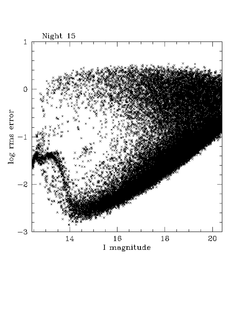
Figure 5: Photometric precision of night 15 of our monitoring run of NGC 6208. In this diagram, slightly more than 5000 stars have photometry of precision 1% or better. This rms is measured as the scatter around the mean magnitude of the star under investigation. The 1%-photometry stars cover a magnitude range of slightly more than 2.5 mags. The “Z”-shaped feature for stars brighter than $I\sim 14$ is due to the onset of saturation for some of the stars in some of the images in the time series. The clustering of stars around log rms $\sim$ 0 is caused by crowding effects when for some of the images, faint stars are blended together with nearby bright stars.

Our $I$-band, high-cadence ($\sim$ 7 min, including 2 min readout time) photometric monitoring enables us to typically attain 1% precision in our relative photometry for around 3000–5000 stars per cluster target field in the range $14.5<I<17$ (see Fig. 5). This number corresponds to a lower limit to the number of stars around which we can detect planetary transits (see §3.1). In the context of outlining our survey strategies, we present some of our preliminary results of the studies of the open clusters NGC 2660 and NGC 6208. In this Section we explain our approach to target selection, specifically designed to maximize the number of target stars of appropriate spectral type.

6.1 Overall Potential Targets

Our potential OC targets listed in Table 1 were chosen with the basic goal that we observe as many cluster member stars as possible at a sufficiently high photometric precision and high-cadence of observations to detect CEGPs around them. Richness classes are given whenever they were available. We note that we used these published richness classes only as a guideline (i.e., we gave extra considerations to OCs classified as rich, but did not necessarily discard any OCs classified as poor) and relied more on visual inspection and photometric analysis of sky survey images of the cluster regions.

Targets in Table 1 were further selected based on the published estimates for distance and foreground reddening. To select a cluster with a suitable distance we consider the preferred range of spectral types (G to M), our adopted relatively short exposure times (see §7.2), and the size of the LCO Swope telescope.

As an example of how distance, exposure time, target spectral type, and reddening are related we use our OC NGC 6208. In Fig. 5, we show our photometric precision as a function of $I$ magnitude of our NGC 6208 data (night 15), obtained during May and June 2003 at the LCO 1m Swope Telescope. We conservatively estimate that, with our exposure time of 300s per frame, we attain 1% precision for a range of about 2.5 magnitudes ($14.5<I<17$). From the WEBDA database (see also Table 1) we find that the distance to NGC 6208 is 939 pc, and the foreground reddening is $E_{B-V}=0.210$. Using the relation $A_{I}=1.94E_{B-V}$ from Schlegel et al. (1998), we find that $I=17$ for NGC 6208 cluster members corresponds to $M_{I}=6.73$ which we call $M_{I_{limit}}$ in Table 1. Using table 15.7 in Cox (2000), this corresponds to an MK spectral type of M0 or M1. The bright limit, above which saturation will start to set in, would be at $M_{I}\sim 4.2$ which would correspond to an MK spectral type of approximately G5 (Cox, 2000). Once the range of spectral types for the monitored cluster members is determined, we can estimate the range of planetary radii which would be detectable (see Fig. 1).

6.2 Potential Targets for a Given Observing Run

For a given slot of observing time, we use Table 1 as the source from which we pre-select two or three potential observing targets for the run. The final target selection is then performed based on our own data, taken either during a previous observing run or at the very beginning of the observing run itself (see below). The main criterion at the pre-selection stage is the observability of the potential targets to maximize the time during which we can observe the OC.

With all of the other constraints (distance, reddening, richness) on cluster selection, finding a cluster that is observable all night long becomes challenging when observing runs are long. The main criterion for a successful transit search is maximizing the time during which we can observe the respective target OC (to increase $P_{vis}$), making clusters of numerically high southern declination preferable targets.

6.3 Final Target Selection

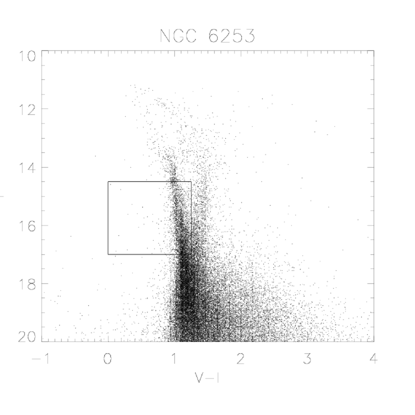
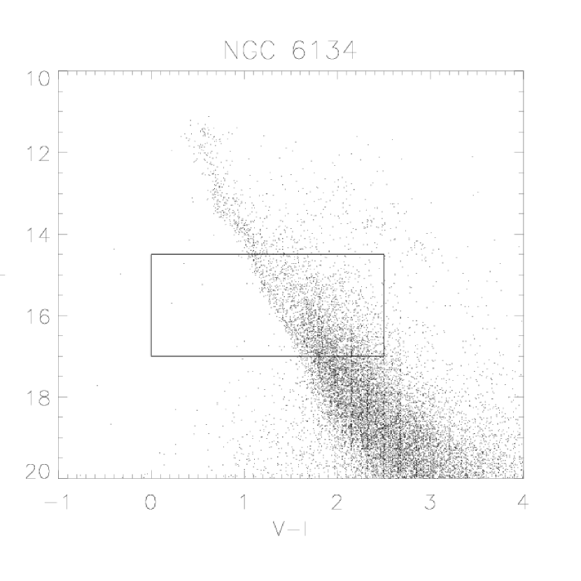
Figure 6: This figure illustrates our approach concerning final target selection, based on our own test data. To choose between the two potential target clusters of different distances and foreground reddening estimates, we counted the number of stars in the boxes (“usable stars”) on the CMDs; the magnitude cuts are conservatively representative of the range within which our monitored stars have photometric rms of less than 1% (see Fig. 5). For NGC 6253, we applied a color cut such that our estimate does not include the evolved background sequence visible in the CMD to the red side of the box at $V-I\sim 1.4$, since transiting planets around evolved stars are not detectable due to the large radius of the parent stars. For NGC 6134, we do not see an evolved background sequence and thus increased the color range to $V-I\sim 2.5$, in part because the foreground reddening estimate is higher for this cluster (see Table 1). We note that saturation of our stars sets in at $I\sim 14.5$. For details, see §6.3. Estimates for “usable” stars for our other OC targets are given in Table 1.

Our final target selection is based on the evaluation of $VI$ test data (see Fig. 6) for the group of pre-selected clusters, involving the following steps:

1. We create (at least roughly) calibrated $VI$ CMDs of the potential target clusters based on our own test data. These data were obtained either during the beginning of the same observing run or during prior runs during photometric conditions and reasonable seeing, and have the same exposure time as for the eventual monitoring. Figure 6 shows these CMDs for the OCs NGC 6253 (left panel) and NGC 6134 (right panel), both of which were targets for our June 2004 run.

2. Within this CMD, we count the number of stars for which we expect to obtain photometry down to 1% or better, which, according to Fig. 5, will include most stars with $14.5<I<17$. Note that we pre-select our targets based on their distance, so that stars within this range of apparent magnitude will be of spectral type G or later.

3. As a final step, we perform cuts in $V-I$ color to eliminate the redder sequence of background evolved disk stars if it is present in the CMD. Stellar radii of evolved stars are significantly larger than their main-sequence counterparts, and thus detecting planets around evolved stars is virtually impossible due to the reduced photometric signal depth of a transiting planet. We show how we eliminate the evolved sequence from consideration in the left panel of Fig. 6.

4. The result of this count approximately corresponds to the number of small main-sequence stars we can monitor at the 1% photometry level and serves as the figure of merit in the cluster selection decision-making process. Since the box in the CMD of NGC 6253 contains more stars (3400) than the one for NGC 6134 (2850), NGC 6253 was chosen as our observing target for June 2004. The last column of Table 1 shows the estimates of the numbers of 1%-rms stars for our potential target clusters which have test data available.

7 EXPLORE/OC Observing Strategy

The EXPLORE/OC observing strategy is designed to maximize $P_{vis}$, minimize false positives, and to constrain field contamination—the issues described in §3 and 4. We review aspects of observing strategy that are most important for our project. Some of these are covered in M03 but are included here for completeness. We focus in particular on considerations necessitated by observing OCs instead of Galactic fields.

7.1 Choice of Filter

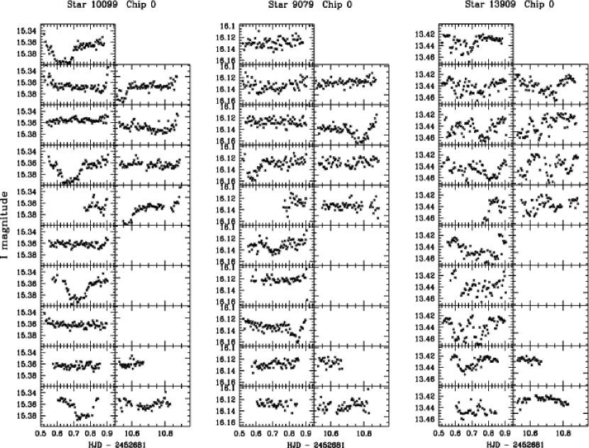
Figure 7: Examples of light curves derived from our high-precision relative photometry (see §8) of our NGC 2660 data. Every panel of one of the light curves represents the data taken during a single night, starting with night 1 on the bottom left. Night 2’s data are shown in the panel directly above it, night 3 above that and so on. No data were obtained during nights 13–15 due to telescope scheduling, and nights 6 and 12 were only partially useful due to weather. All three displayed light curves show the low-amplitude, transit-like signal we are looking for in our survey. They are, however, most likely caused by non-planetary phenomena such as a larger-sized companion (left panel) or grazing binaries (middle and right panels). Our preliminary work on spectral type determination indicates that star 10099 (left panel) is an early G star, star 9079 (middle) is a late A star, and star 13909 (right) is somewhere between F2 and F5.

Our photometric monitoring is done in the $I$-band. The shape of a transit in the photometric light curve is dependent on the filter due to the color dependence of limb darkening whose effects are smaller in $I$ than in the bluer bands. (see §2 and figure 2 in M03). The transit depth is near constant in $I$ when the planet is fully superimposed on the parent star. Because of this “flat-bottomed” light curve in $I$, the shape of the transit makes it easier to distinguish planet transits from the signal caused by grazing binaries (basically a ‘pointy’ or ‘round’ eclipse instead of a flat-bottomed one) than at bluer bands where limb darkening is stronger. Fig. 7 shows a light curve with a flat-bottomed eclipse, illustrating that flat bottoms do indeed occur at I-band.

Additional advantages of observing in the $I$-band are (a) increased sensitivity to redder, intrinsically smaller stars which offer greater chances of detecting orbiting CEGPs, and (b) suffering less extinction due to dust than in the bluer bands.

Disadvantages may include (a) lower CCD quantum efficiency in the $I$-band compared to, e.g., the $R$-band, and (b) the occurrence of fringing due to multiple reflections and subsequent interference internal to the CCD substrate or between the supporting substrate and the silicon. Fringing is usually more visible in $I$ than in $BVR$, due to the abundant night sky emission lines in the $I$ wavelength range. We note that we do not encounter any fringing at all with our setup at the Swope Telescope at LCO.

We also do not change filters during OC monitoring since such a strategy would effectively reduce our observing cadence (§7.2).

7.2 Single-Cluster/High-Cadence Observing

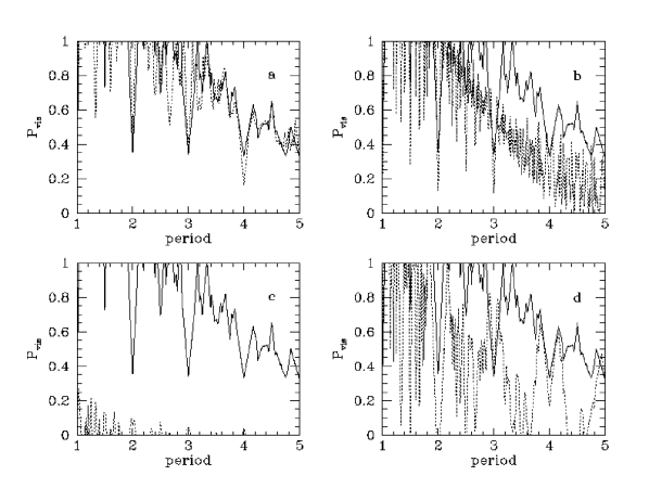
Figure 4: Dependence of $P_{vis}$ upon period (days) when using different observing strategies. The solid line in all four panels corresponds to $P_{vis}$ (two full transits) of a 20-night (10.8h) uninterrupted observing run. In Panel a, the dotted line corresponds to $P_{vis}$ of a 40-nights observing run during which we only observe the first two out of every four nights. $<P_{vis}>$ (periods between 1 and 5 days) of the 20-night observing run is 0.681. $<P_{vis}>$ for the 2-nights-on, 2-nights-off strategy over 40 nights is 0.666. The dotted line in Panel b shows $<P_{vis}>$ when observing the first half of every night for 40 nights in a row: $<P_{vis}>\sim$ 0.437. When observing a third of every night for 60 nights, as shown by the dotted line in Panel c, $<P_{vis}>$ goes down to 0.007. Finally, Panel d illustrates the aliasing effect of only observing 2 out of 4 nights. The dotted line represents the probability of two observed transits being consecutive, as a function of period. Averaged over all periods, only about half of all detected pairs of transits would be consecutive when following the 2-nights-on, 2-nights-off strategy. Note that these numbers are slight overestimates (few percent) because they do not account for the drift of sidereal time that would affect a specific target’s observability. For details, see text (§7).

In order to maximize the chance of detecting any existing planetary transits, we do not alternate OC targets (even though we would increase the number of monitored stars that way) but instead observe the same cluster for as many hours as possible during the night (Figures 3 and 4). The main reason for this strategy is to conduct high-cadence observing.

The main goal of this approach is to distinguish a true transit light curve from false positives such as grazing eclipsing binary stars, an M-star eclipsing a larger star, or stellar blends (Seager & Mallén-Ornelas, 2003; Charbonneau et al., 2004). Because the total duration of a short-period planet transit is typically a few hours, with ingress and egress as little as 20 minutes, high-cadence observing is essential for well-resolved light curves for a limited-duration observing run where only two or three transits are expected. A well-resolved light curve with good photometric precision can be used to derive astrophysical parameters of the planet-star system from the light curve alone (e.g., Seager & Mallén-Ornelas, 2003) which is useful in both ruling out subtle false positives such as blended eclipsing binaries, and in obtaining an estimate of planet radius. In particular, the density of the parent star is of interest for distinguishing between a planetary transit in front of a main-sequence star, and the case of a late-type dwarf orbiting a giant star. The star’s density, however, (1) can only be calculated from photometry data alone when assuming a stellar mass-radius relation, and (2) is sensitively dependent on the full duration of the transit (including ingress and egress), and the duration of totality only.

The flatness of a light curve during the out-of-eclipse stages of a system offers another means of separating planetary transits from stellar eclipses, as illustrated in Sirko & Paczyński (2003) and Drake (2003). Short-period binary stars will have gravitationally distorted, non-spherical shapes which will result in a constant sinusoidal brightness variation of the light curve with a maximum at quadrature.

We also do not change targets during the course of an observing run of $\sim$20 nights or less (see Fig. 2). The justification for this strategy is simple: to maximize $P_{vis}$. From Panel b of Fig. 2, one can see that the typical values for $<P_{vis}>$ ($P_{vis}$ averaged over all periods between 1 and 5 days) of a $\sim$ 20-night observing run with some holes due to weather will reduce the estimated number of detected planets to 50 – 70% of the “theoretical” value as calculated in §3.1. Panel c shows that the efficiency, i.e., how much is added to $<P_{vis}>$ per night, will peak at around 18 nights for perfect conditions, justifying our goal of observing every cluster for around 20 nights in a row.

Alternating cluster targets was suggested by Janes (1996). Street et al. (2003) adopted an alternating cluster strategy, and while their detection algorithm could find transits, they found that having only 4 to 6 data points observed during transit was a limiting factor in both the detection S/N and in discriminating against false positives. Furthermore, while alternating cluster targets may provide more monitored stars, this strategy will favor only the 1- to 2-day period planets if the observing run is not long enough (Figure 3).

Targeting only one cluster during the night further allows us to keep the stars in the targets OCs on our images at exactly the same place on the chip (to within less than 1 arcsec). This helps us simplify the photometry pipeline. In addition, cosmetic problems with the CCD, such as bad columns or bad pixels, will eliminate the same stars in every exposure.

7.3 Dynamic Observing and Optimization of Available Telescope Time

We use a real-time approach to maximizing $P_{vis}$ if the allocated observing time is significantly larger than 20 nights, e.g., $\geq$ 30 nights, based on detecting a single, full transit.

Panel b of Fig. 2 illustrates that the probability of detecting an existing single transit (dashed line) will reach about 65–70% after around 10 nights of continuous observing with 10.8 hours per night. As our data reduction pipeline allows us to do practically real-time data reduction, we can inspect our highest-quality light curves for the existence of a single transit after around 10 nights. If, at that point, we do not see any indication of a single transit anywhere in our data, we will move on to the next target and observe it for the remainder of the allocated time. This approach is essentially a comparison of probabilities: the probability of detecting two transits in a new cluster in the remaining observing time versus the probability (given no transits observed so far) of detecting two transits in the current cluster if we monitor it for the rest of the available observing time.

7.4 Different Observing Strategies

In this Section, we describe how different arrangements of observing nights affect $P_{vis}$.

At private observatories (such as LCO), different longer-term projects requiring many nights may compete for time at smaller telescopes such that their allocation of nights needs to be split. We explain below how different ways of dividing observing time between our project and others affects our likelihood of detecting existing planetary transits.

In Fig. 4, we illustrate the efficiency of a number of different observing strategies which may result from such split-time arrangements. The solid line in all four panels corresponds to $P_{vis}$ (2 transits detected) of an observing run of 20 uninterrupted nights with 10.8 hours of observing each night.

In Panel a, the dotted line corresponds to $P_{vis}$ of an observing run spread over 40 nights (10.8 hours per night), during which we observe only for the first two nights out of every four. $P_{vis}$ is approximately the same as the one for 20 consecutive nights. The $P_{vis}$ averaged over all periods (1 day – 5 days), $<P_{vis}>$, of the 20-consecutive-nights observing run is 0.681. The same $<P_{vis}>$ for the 2-nights-on, 2-nights-off strategy over 40 nights is 0.666. We note that the 2-on, 2-off strategy may impose difficulties in (1) the period determination due to aliasing effects (see below), and (2) the loss of observing time per night due to the drift of the sidereal time over the course of such a long observing run.

In Panel b, the dotted line showcases the result of observing only the first half of every night for 40 nights in a row. The likelihood of detecting existing transits is reduced significantly ($<P_{vis}>\sim$ 0.437). For a strategy of observing a third of every night for 60 nights, as shown by the dotted line in Panel c, $<P_{vis}>$ goes down to 0.007.

Note that none of these numbers takes into account the drift of the sidereal time which would reduce the number of hours of observability during the night as a function of declination of the target. As a result of the sidereal drift, $<P_{vis}>$ would be reduced from 0.748 for a run of 20 consecutive nights to 0.705 for a run of 40 nights with the 2-nights-on, 2-nights-off strategy for NGC 6208, assuming it is perfectly centered in RA at the midpoint of the hypothetical observing run. We calculated similar decreases (on the order of 5% or less) in $<P_{vis}>$ when comparing the two observing strategies for the other clusters in Table 1.

Finally, Panel d illustrates the aliasing effect of only observing 2 out of 4 nights. The dotted line in Panel d corresponds to the probability of detecting two existing transits from which the period can be correctly determined when applying the 2-nights-on, 2-nights-off strategy over the course of 40 nights. $<P_{vis}>$ of the dotted line is 0.356, meaning that only about half (0.356/0.666) of all transit observations would result in a correct calculation of the period, whereas the rest would suffer from aliasing effects. Note that this ratio is sensitively dependent on the period itself, as illustrated by the dotted line. For comparison, a strategy of 1-night-on, 1-night-off would produce $<P_{vis}>$ (two transits observed) of 0.677, but a $<P_{vis}>$ (no aliasing) of only 0.286, meaning that a larger fraction (1-(0.286/0.677)$\simeq 58$%) of observed transits would result in an incorrect calculation of the period. The strategy of continuously observing for 20 nights will give a $<P_{vis}>$ (no aliasing) of 0.406, i.e., an correct estimate of the period in 0.406/0.682$\sim$60% of the cases.

We thus conclude that while having 20 consecutive, uninterrupted nights is clearly the most favorable solution, we can tolerate the strategy where we observe 2 out of every four nights without a significant loss in $<P_{vis}>$, but which will increase the probability of aliasing effects in the period determination.

7.5 Contamination by Galactic Field Stars

Estimates of background or foreground stellar contamination to OCs are valuable since they are the basis upon which statistical estimates of planet frequency among OC members are based, regardless of whether a planet was detected or not. In order to get a handle on contamination, we observe two control fields per target cluster at the same Galactic latitude, approximately a degree away from the OC. These observations are ideally taken in $V$ and $I$, using the same exposure time as for the cluster field, and taken in the same weather and seeing conditions. To first order, the excess number of stars in the cluster field will be representative of the number of cluster members, subject, of course, to uncertainty due to fluctuations of background and foreground star counts.

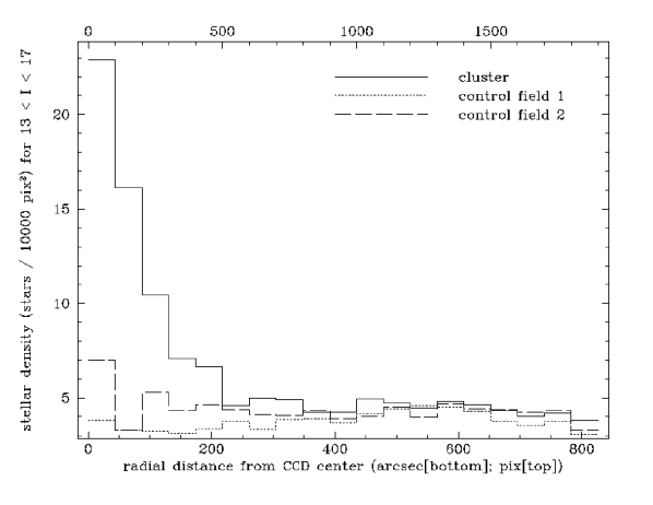
Figure 8: This figure compares the stellar density (measured in stars per 100 pix $\times$ 100 pix on the CCD with $13.0<I<17.0$) as a function of radial distance from the CCD center of the NGC 2660 open cluster image (solid line) and two control fields (dotted and dashed lines) at the same Galactic latitude offset by 1 degree in the sky in either direction in Galactic longitude. The contamination is around 80% over the whole field of the CCD, and approximately 30% for the inner $\sim$ 4 arcmin. For details, see §7.5.

Figures 8 and 9 show this approach for estimating contamination for the observed OC NGC 2660. Fig. 8 compares the stellar density (measured in units of stars per 100 pix $\times$ 100 pix on the CCD with $13.0<I<17.0$) as a function of radial distance from the CCD center of the cluster image of NGC 2660 (solid line) and two control fields (dotted and dashed lines) at the same Galactic latitude offset by 1 degree in the sky in either direction. The comparison between the CMDs of the cluster and control fields is shown in Fig. 9. Although the cluster main sequence is not clearly visible in its CMD, one may nevertheless see a higher density of stars with respect to the control field CMDs at colors red-ward of $V-I\sim 1.2$, as well as a red clump at around $I\sim 13$ and $V-I\sim 1.4$. The total number of stars within $13.0<I<17.0$ in the cluster field is around 3500 stars versus 2700 and 2900 stars in the two control fields. The contamination over the entire CCD field is thus around 80%, and approximately 30% towards the center of the field out to a distance of around 4 arcmin.

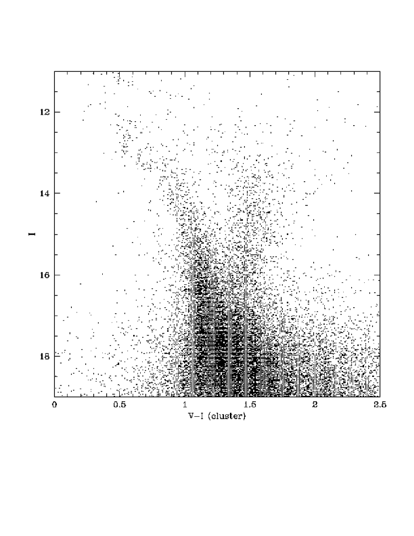
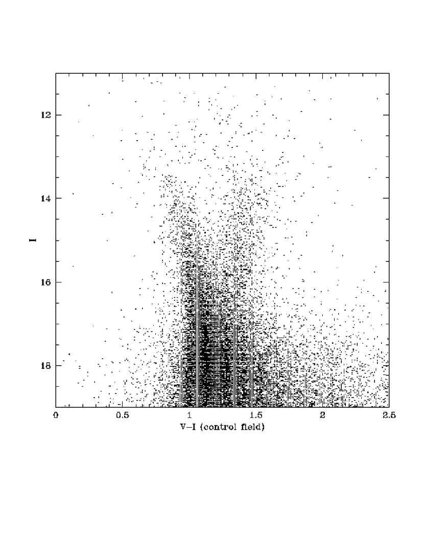
Figure 11: This figure shows the CMDs of the field centered on NGC 6208 (left panel) and a control field (right panel) at the same Galactic latitude offset by 1 degree in the sky. The comparison between the CMDs shows a slight excess of stars in the cluster CMD at bright magnitudes. These excess stars (located around $I\sim 13.0,V-I\sim 0.7$) are evenly distributed over the cluster field, and are approaching the bright limit of our photometry (see Fig. 5). Previous studies (Lindoff, 1972; Paunzen & Maitzen, 2001) already mentioned the difficulty in separating the cluster main sequence from the Galactic disk population. For details, see §7.5.

Figures 10 and 11 illustrate how much more severe this contamination can be, using NGC 6208 as an example (for which we only have data for a single control field). Fig. 10 compares the stellar density (same units as Fig. 8) as a function of radial distance from the CCD center of the cluster image of NGC 6208 and a control field at the same Galactic latitude offset by 1 degree in the sky. Here, the cluster excess stars do not seem to be very centrally concentrated (cf. Fig. 8). Finally, the comparison between the CMDs of the cluster and control field show a slight excess of stars in the cluster CMD at bright magnitudes (Fig. 11). These excess stars (located around $I\sim 13.0,V-I\sim 0.7$) are evenly distributed over the cluster field, and are approaching the bright limit of our photometry (see Fig. 5). The total number of stars in the above magnitude range in the cluster field is around 6200 stars versus 6000 stars in the control field. This would amount to a contamination of 97% over the entire field, and of around 85% in the inner 5 arcmin. This heavy contamination and the associated high density of the region in which NGC 6208 is located was noticed by Lindoff (1972) and reiterated in Paunzen & Maitzen (2001). This cluster contamination of 97% is similar to the 94% contamination of NGC 6819 estimated by Street et al. (2003). Taking into account this high rate of contamination, only a few hundred stars of high relative photometric precision are actually cluster members. Detecting transits around field stars, however, is still useful in a number of ways, outlined in §1.

8 EXPLORE/OC Photometric Data Reduction Methods and Spectroscopy Follow-Up

The EXPLORE/OC strategies concerning photometric data reduction and spectroscopy follow-up work are described here in a brief, preliminary way. More detailed descriptions will follow along with the presentations of our results of the individual OCs.

8.1 Photometry Data Reduction Pipeline

After the standard IRAF image-processing routines, our stellar photometry for the reduction of individual images is performed by an algorithm which will be described in detail in an upcoming publication (Yee et al. 2004, in preparation), and is outlined in principle in §4.3 of M03. We will only provide a very brief overview here.

At the heart of our aperture photometry algorithm is the accurate placement of the aperture relative to the centroid of the star under investigation. This is an important issue due to the relative brightness of the sky with respect to the monitored stars. To minimize the contribution of sky noise and other systematics, we use a relatively small aperture (2–3 seeing disks), which further improves photometry in the situation of moderate crowding (with star separations of a few seeing disks; see §3.3). To achieve the accurate placement of the aperture crucial for obtaining high-precision relative photometry, we use an iterative sinc-shifting technique to re-sample every star individually such that the central 3 $\times$ 3 pixels are symmetrically located about the centroid of the respective star’s PSF. Performing this shift for every object in the frame is then equivalent to using an identical placement of the aperture masks for every object, ensuring proper relative photometry. With such re-sampling, aperture photometry of different aperture radii can be performed simply by using integer pixel masks of various sizes. Sinc-function re-sampling is an ideal method for shifting an image that is Nyquist sampled since it preserves resolution, noise characteristics, and flux (Hemming, 1977; Yee, 1988).

Our relative photometry is then performed by iteratively determining the most stable stars within subregions of the CCD field. All other stars within the same subregion are shifted to the photometric system of these reference stars, thereby using iterations to minimize the scatter and to remove outliers from the calculation of the photometric shift. The number of iterations, criteria for outlier removal, size of the subregions, and minimum number of stars per subregion are parameters that vary for each dataset. Some of the light curves produced by this algorithm are shown as examples in Fig. 7 and illustrate our potential to detect 1% amplitude signals within the intrinsic scatter of the high-precision photometry for the target magnitude range.

8.2 Spectral Type Determination Follow-Up

We determine spectral types for our planet candidate stars to provide an independent measure of their sizes which may help break degeneracies in the photometric solution such as period aliasing or stellar blends, and may thus determine whether or not costly RV follow-up work is desired (Seager & Mallén-Ornelas, 2003; Torres et al., 2004a, b). We have obtained spectral data using a variety of instruments which include the Boller & Chivens Spectrograph and the IMACS Multi-Object Imaging Spectrograph (both on the Magellan 6.5m Telescopes), as well as the Wide-Field Re-imaging CCD in Grism/Multi-slit mode on the LCO du Pont 2.5m Telescope. We are currently analyzing spectral data for our potential candidates (examples in Fig. 7) from our work on NGC 2660 and NGC 6208 to determine the exact nature of each of the systems. Preliminary results are given in Fig. 7.

Spectral type determination of non-planet-candidate stars in the field will give estimates of the foreground reddening along the line of sight and differential reddening across the field, and provide an independent check on the determination of cluster distance by isochrone fitting. Furthermore, the knowledge of the spectral types of a representative set of stars (tens or hundreds of stars) will provide an additional means of estimating contamination of the sample by Galactic field stars and will allow us to determine the parent sample of non-cluster members.

9 Summary

Open clusters are regarded as suitable planet transit monitoring targets because they represent a relatively large number of coeval stars of the same metallicity located at the same distance (§2). Four groups are now monitoring over a dozen open clusters for short-period transiting planets (see §1).

We reviewed the main challenges facing transit searches (§3 and OC surveys in particular §4). In addition to the difficulties involved in any transit search, they include:

• The relatively low number of stars at high relative photometric precision (1–1.5%) compared to Galactic field surveys of roughly the same magnitude range: $\sim$ 5,000 compared to $\sim$ 50,000 stars respectively (though the difference in field size is not taken into account here). This number is similar to the number of stars obtained by the 6$\times$6 degree² shallow transit surveys of brighter stars.

• The severe contamination by Galactic field stars, up to 97% in our clusters for stars at $13<I<17$.

• Differential reddening may be problematic in fitting isochrones.

Just like for field transit surveys, OC transit surveys need to maximize the number of stars with high photometric precision, maximize the probability to detect an existing transit, and not be swamped by false positive transit signals.

We presented aspects of the EXPLORE/OC planet transit survey design that were considered to meet some of the major challenges facing transit surveys. Target selection is a key aspect to survey design with the number of factors over which to optimize (richness, observability, age, distance, foreground reddening) actually limiting the number of available targets for a given observing time and Galactic location. We choose high-cadence observing in order to sample transits well enough to easily rule out false positives such as grazing eclipsing binaries, and to use the unique solution method (Seager & Mallén-Ornelas, 2003) to estimate planet and star parameters. We have shown that with an adopted exposure time and a given telescope, the distance of the cluster can be chosen to target certain spectral types. For the EXPLORE/OC project we do not alternate OCs in a given observing run but instead remain on one cluster in order to maximize finding planet transits. We have shown that this strategy optimizes the probability to detect an existing transiting planet with periods of 2 – 5 days days if observing runs are around 20 days. The single cluster approach, together with near real-time data reduction, allows us to use our dynamic observing strategy for long observing runs ($>$ 30 nights): if a single full transit is not seen within 10 days, the strategy is to move on to another cluster.

EXPLORE/OC is the only OC planet transit survey operating in the southern hemisphere. We have presented some preliminary data on the OCs NGC 2660 and NGC 6208 in order to illustrate the main challenges facing cluster surveys as well as to illustrate our survey design strategy. Our $I$-band, high-cadence photometric monitoring with the LCO 1m Telescope typically attains 1% precision in our relative photometry for around 3000–5000 stars per OC field in the range $14.5<I<17$ with 5 min exposures. For a cluster at a distance of 1 kpc and $E_{B-V}$ of 0.2, this magnitude range corresponds to a range of spectral types between mid-G to early M. We have obtained data on three additional open clusters: IC 2714, NGC 5316, and NGC 6253, and plan to target 4–5 more clusters.

With the $\sim$12 OCs currently being monitored and analyzed by the four existing OC surveys, there is a good chance that some short-period planets will be detected in the near future. Because of the potentially large contamination, and poor availability of physical data on many clusters in the literature, any detected planets should individually be confirmed as cluster members. Furthermore, characterizing of the cluster parameters is important (Burke et al., 2004). With a limited number of stars per cluster, severe contamination from field stars, and considering the finite magnitude range for which high-precision photometry can be obtained, only several hundred to a few thousand cluster members are monitored with high enough photometric precision to detect planet transits; nevertheless, planet transits detected in the contaminating field stars are also useful. If one optimizes the important selection criteria, partly due to the paucity of old clusters, most of the suitable OCs for photometric planet searches and radial-velocity follow up can be searched with a reasonable amount of time and effort.

Table 1: Potential Open Cluster Targets

Cluster	$D$ (pc)	$E_{B-V}$	$M_{I_{limit}}$	$\alpha_{2000}$	$\delta_{2000}$	l	b	[Fe/H]	log(age)	richness	1%-rms stars
NGC 2423	766	0.097	7.39	07 37 06.7	–13 52 17	230.5	3.5	+0.14	8.867	4	1400
NGC 2437	1375	0.154	6.01	07 41 46.8	–14 48 36	231.9	4.1	+0.06	8.390		1600
NGC 2447	1037	0.046	6.83	07 44 29.2	–23 51 11	240.0	0.1	+0.03	8.588	4	1900
NGC 2482	1343	0.093	6.18	07 55 10.3	–24 15 17	241.6	2.0	+0.12	8.604	2
NGC 2539	1363	0.082	6.17	08 10 36.9	–12 49 14	233.7	11.1	+0.14	8.570
NGC 2546	919	0.134	6.92	08 12 15.6	–37 35 40	254.9	–2.0	+0.12	7.874	3	1900
NGC 2571	1342	0.137	6.09	08 18 56.3	–29 44 57	249.1	3.6	+0.08	7.488
NGC 2660	2826	0.313	4.14	08 42 38.0	–47 12 00	265.9	–3.0	–0.18	9.033	5	2750
IC 2488	1134	0.231	6.28	09 27 38.2	–57 00 25	277.8	–4.4	+0.10	8.113		1600
NGC 3114	911	0.069	7.07	10 02 29.5	–60 07 50	283.3	–3.9	+0.02	8.093	2	2900
IC 2714	1238	0.341	5.87	11 17 27.3	–62 43 30	292.4	–1.8	–0.01	8.542		2750
NGC 5316	1215	0.267	6.06	13 53 57.2	–61 52 00	310.2	0.1	+0.13	8.202	3	2800
NGC 5822	917	0.150	6.90	15 04 21.2	–54 23 47	321.6	3.6	–0.03	8.821	4	2600
NGC 6025	756	0.159	7.30	16 03 17.7	–60 25 53	324.6	–5.9	+0.23	7.889	3
NGC 6067	1417	0.380	5.51	16 13 11.0	–54 13 08	329.7	–2.2	+0.14	8.076
NGC 6087	891	0.175	6.91	16 18 50.5	–57 56 04	327.7	–5.4	–0.01	7.976	3
NGC 6134	913	0.395	6.43	16 27 46.5	–49 09 04	334.9	–0.2	+0.18	8.968	4	2850
NGC 6208	939	0.210	6.73	16 49 28.1	–53 43 42	333.8	–5.8	0.00	9.069	4	3250
NGC 6253	1510	0.200	5.72	16 59 05.1	–52 42 32	335.5	–6.3	+0.36	9.70		3400
NGC 6259	1031	0.498	5.97	17 00 45.4	–44 39 18	342.0	–1.5	+0.02	8.336
IC 4651	888	0.116	7.03	17 24 42.0	–49 57 00	340.1	–7.9	+0.09	9.057	4
NGC 6425	778	0.399	6.77	17 47 01.6	–31 31 46	357.9	–1.6	+0.07	7.347	2

Note. — This table shows our previously observed OCs plus a number of potential target clusters which we chose based on the criteria outlined in §5 and §6. Data were taken from the WEBDA database; metallicities from Twarog et al. (1997), available at http://obswww.unige.ch/webda/feh_twarog.html. The column headers are cluster name, distance in parsecs, foreground reddening, limiting absolute $I$ magnitude, $\alpha$, $\delta$, Galactic longitude, Galactic latitude, metallicity, logarithm of the age (in years), the value for the estimated richness class, and the approximate number of stars in the field with relative photometric precision of 1% or better.

figures/vonBraun.fig10a.epsfigures/vonBraun.fig10b.epsfigures/vonBraun.fig10c.eps

Figure 9: This figure shows the CMDs of the field centered on NGC 2660 (left panel) and two control field (middle and right panel) at the same Galactic latitude offset by 1 degree in the sky.

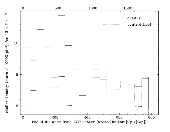
Figure 10: This figure compares the stellar density (measured in stars per 100 $\times$ 100 pix on the CCD with $13.0<I<17.0$) as a function of radial distance from the CCD center of the NGC 6208 open cluster image (solid line) and a control field (dotted line) at the same Galactic latitude offset by 1 degree in the sky. The contamination is around 97% when integrated over the entire CCD, and around 85% towards the inner 5 arcmin. For details, see §7.5.

References

- Alonso et al. (2004) Alonso, R., Brown, T. M., Torres, G., Latham, D. W., Sozzetti, A., Mandushev, G., Belmonte, J. A., Charbonneau, D., Deeg, H. J., Dunham, E. W., O’Donovan, F. T., & Stefanik, R. P. 2004, ArXiv Astrophysics e-prints (astro-ph/0408421)
- Baraffe et al. (2003) Baraffe, I., Chabrier, G., Barman, T. S., Allard, F., & Hauschildt, P. H. 2003, A&A, 402, 701
- Borucki & Summers (1984) Borucki, W. J. & Summers, A. L. 1984, Icarus, 58, 121
- Bouchy et al. (2004) Bouchy, F., Pont, F., Santos, N. C., Melo, C., Mayor, M., Queloz, D., & Udry, S. 2004, ArXiv Astrophysics e-prints (astro-ph/0404264)
- Bramich et al. (2003) Bramich, D. M., Horne, K. D., & Bond, I. A. 2003, ArXiv Astrophysics e-prints (astro-ph/0310848)
- Brown (2003) Brown, T. M. 2003, ApJ, 593, L125
- Brown et al. (2001) Brown, T. M., Charbonneau, D., Gilliland, R. L., Noyes, R. W., & Burrows, A. 2001, ApJ, 552, 699
- Bruntt et al. (2003) Bruntt, H., Grundahl, F., Tingley, B., Frandsen, S., Stetson, P. B., & Thomsen, B. 2003, ArXiv Astrophysics e-prints (astro-ph/0308072)
- Burke et al. (2003) Burke, C. J., Depoy, D. L., Gaudi, B. S., & Marshall, J. L. 2003, in ASP Conf. Ser. 294: Scientific Frontiers in Research on Extrasolar Planets, 379–382
- Burke et al. (2004) Burke, C. J., Gaudi, B. S., DePoy, D. L., Pogge, R. W., & Pinsonneault, M. H. 2004, ArXiv Astrophysics e-prints (astro-ph/0312083)
- Burrows et al. (2000) Burrows, A., Guillot, T., Hubbard, W. B., Marley, M. S., Saumon, D., Lunine, J. I., & Sudarsky, D. 2000, ApJ, 534, L97
- Butler et al. (2002) Butler, R. P., Marcy, G. W., Vogt, S. S., Tinney, C. G., Jones, H. R. A., McCarthy, C., Penny, A. J., Apps, K., & Carter, B. D. 2002, ApJ, 578, 565
- Cardelli et al. (1989) Cardelli, J. A., Clayton, G. C., & Mathis, J. S. 1989, ApJ, 345, 245
- Carraro & Munari (2004) Carraro, G. & Munari, U. 2004, MNRAS, 347, 625
- Charbonneau (2003) Charbonneau, D. 2003, ArXiv Astrophysics e-prints (astro-ph/0302216)
- Charbonneau et al. (2004) Charbonneau, D., Brown, T. M., Dunham, E. W., Latham, D. W., Looper, D. L., & Mandushev, G. 2004, ArXiv Astrophysics e-prints (astro-ph/0401063)
- Charbonneau et al. (2000) Charbonneau, D., Brown, T. M., Latham, D. W., & Mayor, M. 2000, ApJ, 529, L45
- Charbonneau et al. (2002) Charbonneau, D., Brown, T. M., Noyes, R. W., & Gilliland, R. L. 2002, ApJ, 568, 377
- Cox (2000) Cox, A. N. 2000, Allen’s Astrophysical Quantities (Allen’s Astrophysical Quantities, 4th ed. Publisher: New York: AIP Press; Springer, 2000. Edited by Arthur N. Cox. ISBN: 0387987460)
- Donahue (1998) Donahue, R. A. 1998, in ASP Conf. Ser. 154: Cool Stars, Stellar Systems, and the Sun, 1235
- Drake (2003) Drake, A. J. 2003, ApJ, 589, 1020
- Eggenberger et al. (2004) Eggenberger, A., Udry, S., & Mayor, M. 2004, ArXiv Astrophysics e-prints (astro-ph/0402664)
- Fischer & Valenti (2003) Fischer, D. A. & Valenti, J. A. 2003, in ASP Conf. Ser. 294: Scientific Frontiers in Research on Extrasolar Planets, 117–128
- Friel (1995) Friel, E. D. 1995, ARA&A, 33, 381
- Gaudi (2000) Gaudi, B. S. 2000, ApJ, 539, L59
- Gaudi et al. (2002) Gaudi, B. S., Burke, C. J., DePoy, D. L., Marshall, J. L., Pogge, R. W., & STEPSS Collaboration. 2002, Bulletin of the American Astronomical Society, 34, 1264
- Gilliland et al. (2000) Gilliland, R. L., Brown, T. M., Guhathakurta, P., Sarajedini, A., Milone, E. F., Albrow, M. D., Baliber, N. R., Bruntt, H., Burrows, A., Charbonneau, D., Choi, P., Cochran, W. D., Edmonds, P. D., Frandsen, S., Howell, J. H., Lin, D. N. C., Marcy, G. W., Mayor, M., Naef, D., Sigurdsson, S., Stagg, C. R., Vandenberg, D. A., Vogt, S. S., & Williams, M. D. 2000, ApJ, 545, L47
- Guillot & Showman (2002) Guillot, T. & Showman, A. P. 2002, A&A, 385, 156
- Hemming (1977) Hemming, R. W. 1977, Digital Filtering (Prentice Hall, Englewood Cliffs)
- Henry et al. (2000) Henry, G. W., Marcy, G. W., Butler, R. P., & Vogt, S. S. 2000, ApJ, 529, L41
- Horne (2003) Horne, K. 2003, in ASP Conf. Ser. 294: Scientific Frontiers in Research on Extrasolar Planets, 361–370
- Houdashelt et al. (2000) Houdashelt, M. L., Bell, R. A., & Sweigart, A. V. 2000, AJ, 119, 1448
- Janes (1996) Janes, K. 1996, J. Geophys. Res., 101, 14853
- Janes & Adler (1982) Janes, K. & Adler, D. 1982, ApJS, 49, 425
- Kane et al. (2004) Kane, S. R., Cameron, A. C., Horne, K., James, D., Lister, T. A., Pollacco, D. L., Street, R. A., & Tsapras, Y. 2004, ArXiv Astrophysics e-prints (astro-ph/0406270)
- Konacki et al. (2003a) Konacki, M., Torres, G., Jha, S., & Sasselov, D. D. 2003a, Nature, 421, 507
- Konacki et al. (2003b) Konacki, M., Torres, G., Sasselov, D. D., & Jha, S. 2003b, ApJ, 597, 1076
- Konacki et al. (2004) Konacki, M., Torres, G., Sasselov, D. D., Pietrzynski, G., Udalski, A., Jha, S., Ruiz, M. T., Gieren, W., & Minniti, D. 2004, ArXiv Astrophysics e-prints (astro-ph/0404541)
- Kotredes et al. (2003) Kotredes, L., Charbonneau, D., Looper, D. L., & O’Donovan, F. T. 2003, ArXiv Astrophysics e-prints (astro-ph/0312432)
- Lebreton et al. (2001) Lebreton, Y., Fernandes, J., & Lejeune, T. 2001, A&A, 374, 540
- Lee et al. (2004) Lee, B. L., von Braun, K., Mallén-Ornelas, G., Yee, H. K. C., Seager, S., & Gladders, M. D. 2004, in American Institute of Physics Conference Series 713: The Search for Other Worlds, 177
- Lindoff (1972) Lindoff, U. 1972, A&AS, 7, 231
- Lynga (1995) Lynga, G. 1995, VizieR Online Data Catalog, 7092, 0
- Mallén-Ornelas et al. (2003) Mallén-Ornelas, G., Seager, S., Yee, H. K. C., Minniti, D., Gladders, M. D., Mallén-Fullerton, G. M., & Brown, T. M. 2003, ApJ, 582, 1123 (M03)
- Marcy et al. (2004) Marcy, G. W., Butler, R. R., Fischer, D. A., & Vogt, S. S. 2004, in XIXth IAP Colloquium, Extrasolar Planets: Today and Tomorrow, held in Paris, June 30 - July 4, 2003, ASP Conference Series
- Mazeh et al. (2000) Mazeh, T., Naef, D., Torres, G., Latham, D. W., Mayor, M., Beuzit, J., Brown, T. M., Buchhave, L., Burnet, M., Carney, B. W., Charbonneau, D., Drukier, G. A., Laird, J. B., Pepe, F., Perrier, C., Queloz, D., Santos, N. C., Sivan, J., Udry, S., & Zucker, S. 2000, ApJ, 532, L55
- Mermilliod (1996) Mermilliod, J.-C. 1996, in ASP Conf. Ser. 90: The Origins, Evolution, and Destinies of Binary Stars in Clusters, 475
- Mighell et al. (1998) Mighell, K. J., Sarajedini, A., & French, R. S. 1998, AJ, 116, 2395
- Mochejska et al. (2002) Mochejska, B. J., Stanek, K. Z., Sasselov, D. D., & Szentgyorgyi, A. H. 2002, AJ, 123, 3460
- Mochejska et al. (2004) Mochejska, B. J., Stanek, K. Z., Sasselov, D. D., Szentgyorgyi, A. H., Westover, M., & Winn, J. N. 2004, ArXiv Astrophysics e-prints (astro-ph/0402309)
- Munari & Carraro (1996) Munari, U. & Carraro, G. 1996, MNRAS, 283, 905
- Naef et al. (2004) Naef, D., Mayor, M., Beuzit, J. L., Perrier, C., Queloz, D., Sivan, J. P., & Udry, S. 2004, ArXiv Astrophysics e-prints (astro-ph/0409230)
- Nilakshi et al. (2002) Nilakshi, N., Sagar, R., Pandey, A. K., & Mohan, V. 2002, A&A, 383, 153
- Nordstroem et al. (1997) Nordstroem, B., Andersen, J., & Andersen, M. I. 1997, A&A, 322, 460
- O’Donovan et al. (2003) O’Donovan, F. T., Charbonneau, D., & Kotredes, L. 2003, ArXiv Astrophysics e-prints (astro-ph/0312289)
- O’Donovan et al. (2004) —. 2004, in American Institute of Physics Conference Series 713: The Search for Other Worlds, 169
- Pace & Pasquini (2004) Pace, G. & Pasquini, L. 2004, ArXiv Astrophysics e-prints (astro-ph/0406651)
- Paulson et al. (2004) Paulson, D. B., Saar, S. H., Cochran, W. D., & Henry, G. W. 2004, AJ, 127, 1644
- Paunzen & Maitzen (2001) Paunzen, E. & Maitzen, H. M. 2001, A&A, 373, 153
- Perryman et al. (1998) Perryman, M. A. C., Brown, A. G. A., Lebreton, Y., Gomez, A., Turon, C., de Strobel, G. C., Mermilliod, J. C., Robichon, N., Kovalevsky, J., & Crifo, F. 1998, A&A, 331, 81
- Pont et al. (2004) Pont, F., Bouchy, F., Queloz, D., Santos, N., Melo, C., Mayor, M., & Udry, S. 2004, ArXiv Astrophysics e-prints
- Prisinzano et al. (2004) Prisinzano, L., Micela, G., Sciortino, S., & Favata, F. 2004, A&A, 417, 945
- Queloz et al. (2001) Queloz, D., Henry, G. W., Sivan, J. P., Baliunas, S. L., Beuzit, J. L., Donahue, R. A., Mayor, M., Naef, D., Perrier, C., & Udry, S. 2001, A&A, 379, 279
- Raboud et al. (1997) Raboud, D., Cramer, N., & Bernasconi, P. A. 1997, A&A, 325, 167
- Richardson et al. (2003a) Richardson, L. J., Deming, D., & Seager, S. 2003a, ApJ, 597, 581
- Richardson et al. (2003b) Richardson, L. J., Deming, D., Wiedemann, G., Goukenleuque, C., Steyert, D., Harrington, J., & Esposito, L. W. 2003b, ApJ, 584, 1053
- Rosvick & Balam (2002) Rosvick, J. M. & Balam, D. 2002, AJ, 124, 2093
- Sandrelli et al. (1999) Sandrelli, S., Bragaglia, A., Tosi, M., & Marconi, G. 1999, MNRAS, 309, 739
- Schlegel et al. (1998) Schlegel, D. J., Finkbeiner, D. P., & Davis, M. 1998, ApJ, 500, 525
- Seager & Mallén-Ornelas (2003) Seager, S. & Mallén-Ornelas, G. 2003, ApJ, 585, 1038
- Sirko & Paczyński (2003) Sirko, E. & Paczyński, B. 2003, ApJ, 592, 1217
- Street et al. (2002) Street, R. A., Horne, K., Lister, T. A., Penny, A., Tsapras, Y., Quirrenbach, A., Safizadeh, N., Cooke, J., Mitchell, D., & Collier Cameron, A. 2002, MNRAS, 330, 737
- Street et al. (2003) Street, R. A., Horne, K., Lister, T. A., Penny, A. J., Tsapras, Y., Quirrenbach, A., Safizadeh, N., Mitchell, D., Cooke, J., & Cameron, A. C. 2003, MNRAS, 340, 1287
- Torres et al. (2004a) Torres, G., Konacki, M., Sasselov, D. D., & Jha, S. 2004a, ApJ, 609, 1071
- Torres et al. (2004b) —. 2004b, ArXiv Astrophysics e-prints (astro-ph/0406627)
- Twarog et al. (1997) Twarog, B. A., Ashman, K. M., & Anthony-Twarog, B. J. 1997, AJ, 114, 2556
- Udalski et al. (2002a) Udalski, A., Paczynski, B., Zebrun, K., Szymanski, M., Kubiak, M., Soszynski, I., Szewczyk, O., Wyrzykowski, L., & Pietrzynski, G. 2002a, Acta Astronomica, 52, 1
- Udalski et al. (2003) Udalski, A., Pietrzynski, G., Szymanski, M., Kubiak, M., Zebrun, K., Soszynski, I., Szewczyk, O., & Wyrzykowski, L. 2003, Acta Astronomica, 53, 133
- Udalski et al. (2002b) Udalski, A., Zebrun, K., Szymanski, M., Kubiak, M., Soszynski, I., Szewczyk, O., Wyrzykowski, L., & Pietrzynski, G. 2002b, Acta Astronomica, 52, 115
- Vidal-Madjar et al. (2003) Vidal-Madjar, A., Lecavelier des Etangs, A., Désert, J.-M., Ballester, G. E., Ferlet, R., Hébrard, G., & Mayor, M. 2003, Nature, 422, 143
- Villanova et al. (2004) Villanova, S., Baume, G., Carraro, G., & Geminale, A. 2004, A&A, 419, 149
- von Braun et al. (2004) von Braun, K., Lee, B. L., Mallén-Ornelas, G., Yee, H. K. C., Seager, S., & Gladders, M. D. 2004, in American Institute of Physics Conference Series 713: The Search for Other Worlds, 181
- von Braun & Mateo (2001) von Braun, K. & Mateo, M. 2001, AJ, 121, 1522
- von Hippel et al. (2002) von Hippel, T., Steinhauer, A., Sarajedini, A., & Deliyannis, C. P. 2002, AJ, 124, 1555
- Weldrake et al. (2003) Weldrake, D. T. F., Sackett, P. D., & Bridges, T. J. 2003, ArXiv Astrophysics e-prints (astro-ph/0309476)
- Weldrake et al. (2004) Weldrake, D. T. F., Sackett, P. D., Bridges, T. J., & Freeman, K. C. 2004, AJ, 128, 736
- Wright (2004) Wright, J. T. 2004, ArXiv Astrophysics e-prints (astro-ph/0406338)
- Yee (1988) Yee, H. K. C. 1988, AJ, 95, 1331
- Yee et al. (2003) Yee, H. K. C., Mallén-Ornelas, G., Seager, S., Gladders, M., Brown, T. X., Minnitti, D., Ellison, S., & Mallén-Fullerton, G. 2003, in Discoveries and Research Prospects from 6- to 10-Meter-Class Telescopes II. Edited by Guhathakurta, Puragra. Proceedings of the SPIE, Volume 4834, pp. 150-160 (2003), 150–160
- Zucker & Mazeh (2002) Zucker, S. & Mazeh, T. 2002, ApJ, 568, L113