Comparing the temperatures of galaxy clusters from hydro-N-body simulations to Chandra and XMM-Newton observations

Theoretical studies of the physical processes in clusters of galaxies are mainly based on the results of numerical simulations, which in turn are often directly compared to X-ray observations. Although trivial in principle, these comparisons are not always simple. We show that the projected spectroscopic temperature of clusters obtained from X-ray observations is always lower than the emission-weighed temperature. This bias is related to the fact that the emission-weighted temperature does not reflect the actual spectral properties of the observed source. This has implications for the study of thermal structures in clusters, especially when strong temperature gradients, like shock fronts, are present. In real observations shock fronts appear much weaker than what is predicted by emission-weighted temperature maps. We propose a new formula, the spectroscopic-like temperature function that better approximates the spectroscopic temperature, making simulations more directly comparable to observations.

1 Introduction

Recent observational data with high spatial and spectral resolution suggest that clusters are far from isothermal, and show instead a number of peculiar thermal features, like cold fronts [$\!{}^{{\bf?}}$, $\!{}^{{\bf?}}$] cavities [$\!{}^{{\bf?}}$], blobs and filaments [$\!{}^{{\bf?}}$,$\!{}^{{\bf?}}$].

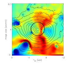
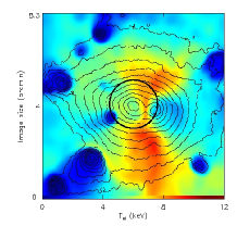
Figure 1: Comparison of the map of the emission-weighted temperature $T_{\rm ew}$  (left-panel) and the spectroscopic-like temperature $T_{\rm sl}$  (right-panel) for the simulated cluster of galaxy. Both maps are obtained by using the gas particles of the hydro-N-body simulation and are binned in $1^{\prime\prime}$ pixels. The contours correspond to the cluster flux.

A theoretical interpretation of these observations clearly requires state-of-the-art hydro-N-body simulations, which can be used to extract realistic temperature maps and/or profiles. The comparison between real and simulated data, however, is complicated by different problems, produced both by projection effects and by instrumental artifacts. A further complication can arise from a possible mismatch between the spectroscopic temperature $T_{\rm spec}$ estimated from X-ray observations and the temperatures usually defined in numerical results. In fact, while $T_{\rm spec}$ is a mean projected temperature obtained by fitting a single or multi-temperature thermal model to the observed photon spectrum, theoretical models fully exploit the three-dimensional thermal information carried by gas particles and so usually define physical temperatures. In the years a number of temperature functions have been introduced in order to compare hydro-N-body simulations with X-ray observations. The most common temperature function used is the so called bolometric emission-weighted temperature function defined as

$$T_{\rm ew}\equiv\frac{\int\Lambda(T)n2TdV}{\int\Lambda(T)n2dV}\ ,$$ (1)

where $\Lambda(T)=\int_{0}^{\infty}\epsilon_{E}dE\propto\sqrt{T}$ (see, e.g., [$\!{}^{{\bf?}}$]). To make observations more directly comparable with simulations we build the software package X-ray Map Simulator (X-MAS) devoted to simulate X-ray observations of galaxy clusters obtained from hydro-N-body simulations [$\!{}^{{\bf?}}$]. Using X-MAS we clearly show that if the cluster has a complex thermal structure the emission-weighted temperature function does not reproduce the spectroscopic estimate and in particular it overestimates this value[$\!{}^{{\bf?}}$]. This problem is illustrated in Fig. 1, Fig. 2, Fig. 3. In fact, in the left panel of Fig 1 we show the emission-weighted temperature map of a simulated cluster that we use as input for X-MAS. We point to the reader the presence in this map of two shock fronts: one in the lower-left corner and the other at the center of the Eastern side of the cluster. In Fig. 2 we show the $T_{\rm spec}$  map derived from the data analysis of a 300 ks Chandra  ACIS-S3 X-MAS “observation” of the cluster shown in Fig 1 (see [$\!{}^{{\bf?}}$] for details).

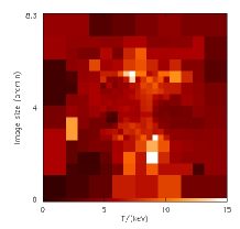
Figure 2: Spectroscopic temperature map of the simulated cluster of galaxy as derived from the spectroscopic analysis of the Chandra  “observation” with the package X-MAS

In order to make a direct comparison of the “observed” temperature map to the emission-weighted one, we decreased the resolution of the latter to match the resolution of the former. Thus, in the left panel of Fig. 3 we report the same map of $T_{\rm ew}$ shown on the left panel of Fig. 1, but re-binned as the map of Fig. 2. To highlight the temperature differences between the $T_{\rm spec}$  and the $T_{\rm ew}$  maps, in the right panel of Fig. 3 we show $(T_{\rm ew}-T_{\rm spec})/T_{\rm spec}$. We only show the pixels where this difference is significant to at least $3\sigma$ confidence level, i.e. $|(T_{\rm ew}-T_{\rm spec})/\sigma_{\rm spec}|>3$. This plot clearly shows that there are many regions where the difference between $T_{\rm ew}$ and $T_{\rm spec}$ is significant to better than $3\sigma$ confidence level. Furthermore, for these pixels the discrepancy ranges from 50 per cent to 200 per cent and even more. Of particular relevance are two cluster regions showing a shock front in the $T_{\rm ew}$  map, in the left panel of Fig. 1: we notice discrepancies of 100-200 per cent, indicating that shock fronts predicted in the $T_{\rm ew}$  map are no longer detected in the observed the $T_{\rm spec}$  map.

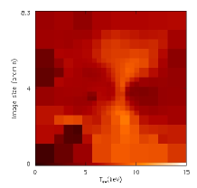
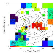
Figure 3: Left panel: emission-weighted temperature map of the simulated cluster of galaxies shown in the left panel of Fig. 1 but re-binned to match the spatial resolution of the spectroscopic temperature map shown in Fig. 2. Right panel: percentile difference between the spectroscopic and emission-weighted temperature maps. In this map we show only the regions where the significance level of the temperature discrepancy is at least $3\sigma$, i.e. $|(T_{\rm ew}-T_{\rm spec})/\sigma_{\rm spec}|>3$, where $\sigma_{\rm spec}$ is the 68 per cent confidence level error associated to $T_{\rm spec}$.

2 A new formula to estimate spectroscopic temperatures

If the cluster thermal structure is complex, the $T_{\rm ew}$ may substantially differ from $T_{\rm spec}$. This is mainly related to the fact that the projected temperature function is not a good physical quantity. From a pure analytic point of view, in fact, the sum of the spectra of two or more thermal model is no longer a thermal model [$\!{}^{{\bf?}}$]. In the real world, however, the finite energy response and limited energy resolution of the X-ray instruments conspire to distort the observed spectra making multi-temperature thermal source spectra fitted by single-temperature thermal models which have little to do with the real temperature, but nevertheless are statistically indistinguishable from it (see [$\!{}^{{\bf?}}$] for details). In [$\!{}^{{\bf?}}$] we show that the temperature that better approximates $T_{\rm spec}$ is given by what we call the “spectroscopic-like” temperature $T_{\rm sl}$. The idea behind the derivation of this temperature function is quite simple: if we assume two thermal components with densities $n_{1}$, $n_{2}$, and temperatures $T_{1}$, $T_{2}$, respectively, requiring matching spectra means that

$$\begin{array}[]{l}n_{1}^{2}\zeta(Z,T_{1})\frac{1}{\sqrt{T}_{1}}\exp(-\frac{E}{kT_{1}})+n_{2}^{2}\zeta(Z,T_{2})\frac{1}{\sqrt{T}_{2}}\exp(-\frac{E}{kT_{2}})\\ \approx A\zeta(Z,T_{\rm sl})\frac{1}{\sqrt{T}_{\rm sl}}\exp(-\frac{E}{kT_{\rm sl}}),\\ \end{array}$$ (2)

where $A$ is an arbitrary normalization constant and $\zeta(Z,T)$ is a parametrization function that accounts for the total Gaunt factor and partly for the line emission.

Both Chandra  and XMM-Newton  are most sensitive to the soft region of the X-ray spectrum, so we expand both sides of Eq. 2 in Taylor series, to the first order in $E/kT$. By equating the zero-th and first-order terms in $E$, assuming a power-law functional form for $\zeta(Z,T_{2})$, and extending to a continuum distribution we find that (see [$\!{}^{{\bf?}}$] for details):

$$\begin{array}[]{rl}T_{\rm sl}&=\frac{\int WTdV}{\int WdV},\\ W&=\frac{n2}{T^{3/4}}.\\ \end{array}$$ (3)

It is interesting to note that $T_{\rm sl}$ weights each thermal component directly by the emission measure but, unlike $T_{\rm ew}$, inversely by their temperature to the power of $3/4$. This means that the observed spectroscopic temperature is biased toward the coolest regions. To prove the quality of $T_{\rm sl}$  in reproducing $T_{\rm spec}$  we do the same test done for $T_{\rm ew}$  and shown in Fig. 3. In the left panel of Fig. 4 we report the cluster $T_{\rm sl}$ map re-binned as the map of Fig. 2. In the right panel of Fig. 4 we show $(T_{\rm sl}-T_{\rm spec})/T_{\rm spec}$. The presence in this map of fewer pixels clearly indicates that the match between $T_{\rm sl}$ and $T_{\rm spec}$  is much better than the one between $T_{\rm spec}$  and $T_{\rm ew}$. Furthermore, most of these pixels shows very small temperature discrepancies. This demonstrates that the $T_{\rm sl}$  temperature gives a much better estimate of the observed $T_{\rm spec}$than the widely used $T_{\rm ew}$.

It is very important to say that, unlike the emission-weighted, the map on the right panel of Fig. 4 does not show big discrepancies between $T_{\rm sl}$  and $T_{\rm spec}$  in both shock regions. This clearly indicate that $T_{\rm sl}$  does a much better job than $T_{\rm ew}$  in predicting the projected spectral properties of such peculiar thermal features.

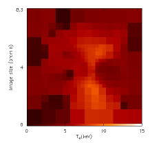
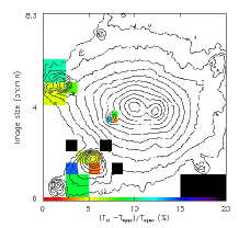
Figure 4: As Fig.  3, but for the spectroscopic-like temperature.

3 Conclusions

The projected $T_{\rm spec}$  of thermally complex clusters is lower than $T_{\rm ew}$. This bias has important implications for the study of thermal structures in clusters like shock fronts. In fact in real observations shock fronts appear much weaker than what is predicted by emission-weighted temperature maps, and may even not be detected. This bias effect is evident on the right panel of Fig. 1 where we report the spectroscopic-like temperature map of the simulated cluster. We notice that the $T_{\rm sl}$ map appears cooler than the map of $T_{\rm ew}$. Furthermore, both shock fronts, which are clearly evident in the $T_{\rm ew}$  map, are no longer detected in the $T_{\rm sl}$ map. This bias may explain why, although numerical simulations predict that shock fronts are a quite common feature in clusters of galaxies, to date there are very few observations of objects in which they are clearly seen. To conclude we stress that the emission-weighted temperature function may give a misleading view of the actual gas temperature structure as obtained from X-ray observations. Thus, here we propose to theoreticians to finally discard its use.

References

References

- [1] M. Markevitch et al. ApJ, 541:542–549, October 2000.
- [2] P. Mazzotta et al. ApJ, 555:205–214, July 2001.
- [3] B. R. McNamara et al. ApJ, 534:L135–L138, May 2000.
- [4] A. C. Fabian et al. MNRAS, 321:L33–L36, February 2001.
- [5] P. Mazzotta, A. C. Edge, and M. Markevitch. ApJ, 596:190–203, October 2003.
- [6] C. S. Frenk et al. ApJ, 525:554–582, November 1999.
- [7] A. Gardini, E. Rasia, P. Mazzotta, G. Tormen, S. De Grandi, and L. Moscardini. MNRAS, in press, astro-ph/0310844, October 2004.
- [8] P. Mazzotta, E. Rasia, L. Moscardini, and G. Tormen. MNRAS, in press, astro-ph/0404425, April 2004.