A 2D analysis of percolation and filamentarity in the SDSS DR1

We have used the Largest Cluster Statistics and the Average Filamentarity to quantify respectively the connectivity and the shapes of the patterns seen in the galaxy distribution in two volume limited subsamples extracted from the equatorial strips of the Sloan Digital Sky Survey (SDSS) Data Release One (DR1). The data was projected onto the equatorial plane and analyzed in two dimensions (2D). Comparing the results with Poisson point distributions at various levels of smoothing we find evidence for a network like topology with filaments being the dominant patterns in the galaxy distribution. With increasing smoothing, a transition from many individual filamentary structures to an interconnected network is found to occur at a filling factor $0.5-0.6$. We have tested the possibility that the connectivity and the morphology of the patterns in the galaxy distribution may be luminosity dependent and find significant evidence for a luminosity-morphology relation, the brighter galaxies exhibiting lowers levels of connectivity and filamentarity compared to the fainter ones. Using a statistical technique, Shuffle, we show that the filamentarity in both the SDSS strips is statistically significant up to $80\,h^{-1}{\rm Mpc}$ but not beyond. Larger filaments, though identified, are not statistically significant. Our findings reaffirm earlier work establishing the filaments to be the largest known statistically significant coherent structures in the universe.

1 Introduction

Quantifying the clustering pattern observed in the galaxy distribution is one of the central themes in modern cosmology. A striking feature visible in all redshift surveys is that the galaxies appear to be distributed along filaments which are interconnected and form a network, often referred to as the “Cosmic Web”. In this paper we quantify the inter-connectivity and the shapes of the patterns seen in the galaxy distribution in the SDSS (York et al. 2000).

The percolation analysis (eg. Shandarin & Zeldovich 1983;Einasto et al. 1984) and the genus statistics (eg. Gott, Dickinson, & Melott 1986) are some of the earliest statistics introduced to quantify the topology of the galaxy distribution. Shandarin & Yess (1998) used the Largest Cluster Statistics (LCS), a percolation technique developed for point-wise distributions, to analyze the connectivity of structures in the Las Campanas Redshift Survey (LCRS; Shectman et al. 1996). The thickness of the six LCRS slices is very small compared to the two other dimensions, and the analysis was carried out on two dimensional (2D) projections. The $\rm LCS$ analysis focuses on the growth of the largest cluster with increasing smoothing. A growth faster than that of a random Poisson point distribution indicates a network topology whereas a slower growth indicates a meatball topology. The $\rm LCS$ analysis shows the presence of a high level of inter-connectivity indicative of a network like structure in the distribution of the LCRS galaxies.

The Minkowski functionals have been suggested as a novel tool to study the morphology of structures in the universe (eg. Mecke, Buchert, & Wagner 1994, Schmalzing & Buchert 1997). Ratios of the Minkowski functionals can be used to define a shape diagnostic ’Shapefinders’ which faithfully quantifies the shapes of both simple and topologically complex objects (Sahni, Sathyaprakash, & Shandarin 1998). Bharadwaj et al. (2000) defined the Shapefinder statistics in 2D, and have used this to demonstrate that the galaxy distribution in the LCRS exhibits a high degree of filamentarity compared to a random Poisson distribution. In a later paper, Bharadwaj et al. (2004) used Shapefinders in conjunction with a statistical technique called Shuffle (Bhavsar & Ling 1988) to determine the maximum length-scale at which the filaments observed in the LCRS are statistically significant. They found that the largest length-scale at which filaments are statistically significant is between $70$ to $80\,h^{-1}$Mpc, for the LCRS $-3^{o}$ slice. Filamentary features longer than $80\,h^{-1}$Mpc, though identified, are not statistically significant. Such features arise from chance alignments of galaxies. Further, for the five other LCRS slices, filaments of lengths $50\,h^{-1}$Mpc to $70\,h^{-1}$Mpc were found to be statistically significant, but not beyond.

The ability to produce the filamentary features observed in redshift surveys is an important test of any model for structure formation. Bharadwaj & Pandey (2004) have used N-body simulations of the $\Lambda{\rm CDM}\,\,$model with a featureless, scale invariant primordial power spectrum and random initial phases to investigate whether the filamentarity predicted by this model is consistent with that detected in the LCRS. They find that the filamentarity in an unbiased $\Lambda{\rm CDM}\,\,$model is less than the LCRS. Introducing a bias $b=1.15$, the model is in rough consistency with the data, and a large bias $(b=1.5)$ which enhances filamentarity at small scales and suppresses it at large scales is ruled out. The filamentarity is very sensitive to the bias , and it may be possible to use a quantitative analysis of filamentarity to determine the bias parameter.

The Sloan Digital Sky Survey (SDSS) offers the possibility of studying coherent structures in the galaxy distribution over length-scales which are substantially larger than possible with earlier surveys like the LCRS. Among the total sky coverage of the publicly available SDSS Data Release One (DR1) are two strips which are centered along the celestial equator ($\delta=0^{\circ}$), one spanning $65^{\circ}$ and the other $91^{\circ}$ in r.a., and their thickness varying within $\mid\delta\mid\leq 2.5^{\circ}$ in dec.. We use galaxies distributed over the redshift range $0.02\leq z\leq 0.2$. The thickness of the three dimensional regions corresponding to these strips is much smaller than the two other dimensions, and we can project the galaxy distribution onto the equatorial plane $(\delta=0)$ without smearing out the large-scale patterns. In this paper we quantify the inter-connectivity and the shapes of the patterns in the resulting 2D galaxy distribution using the same techniques which were earlier applied to the LCRS.

We restrict our analysis to volume limited subsamples described in Section 1 of this paper. The dense sampling of the SDSS allows us to divide the galaxies into two classes based on their luminosities and test if the inter-connectivity and the shapes of the patterns seen in the galaxy distribution are different for the fainter and the brighter galaxies. The large volume of the two SDSS equatorial strips offers further advantages over the LCRS, we discuss these in the appropriate parts of the paper. In this paper we have only considered the average properties of the structures, and we have not addressed questions pertaining to individual filaments, nor have we compared our results to N-body simulations. It is proposed to address these issues in future.

Hoyle et al. (2002) have studied the 2D topology of the SDSS using the genus statistics. In addition to the two equatorial strips used in this paper, they have also used a strip at high declinations. They find that their results are consistent with those from $\Lambda{\rm CDM}\,\,$N-body simulations and also with those from a similar analysis of the 2dFGRS (Hoyle, Vogeley, & Gott 2002). They have also divided the galaxies by colour and separately analyzed them to find that the distribution of the red galaxies shows a shift to a meatball topology relative to the blue galaxies and the full sample, reflecting the fact that red galaxies are distributed in more compact, high density regions. Hikage et al. (2003) have used Minkowski Functionals to study the morphology of the patterns in the galaxy distribution in a preliminary sample from the SDSS. Doroshkevich et al. (2004) have used the Minimal Spanning Tree to identify sheets and filaments in the SDSS DR1. In both these works the authors find their results to be consistent with $\Lambda{\rm CDM}\,\,$N-body simulations.Einasto et al. (2003) have studied the super-cluster void network in the SDSS. Sheth (2004) has used a technique SURFGEN (Sheth et al. 2003) to study the geometry, topology and morphology of the superclusters in mock SDSS catalogues and find that the filamentarity is the dominant morphology of the large superclusters. Shandarin, Sheth, & Sahni (2004) studied the large-scale network in the dark matter density field in N-body simulations from VIRGO consortium using SURFGEN and noticed that the individual superclusters and voids exhibits a significant amount of substructures as indicated by their genus values.

Basilakos, Plionis, & Rowan-Robinson (2001) and Kolokotronis, Basilakos, & Plionis (2002) have studied the super-cluster void network in the PSCz and the Abell/ACO cluster catalogue respectively, finding filamentarity to be the dominant feature. Pimbblet, Drinkwater, & Hawkrigg (2004) performed an analysis of the frequency and distribution of intercluster filaments in the 2dfGRS with a filament classification scheme based on their visual morphology and reported that massive clusters have larger number of filaments.

Traditionally, correlation functions have been used to quantify the statistical properties of the galaxy distribution with the two-point correlation function and its Fourier transform, the power spectrum, receiving most of the attention. For the SDSS this includes analysis of the power spectrum(eg. Szalay et al. 2002; Tegmark et al. 2002; Tegmark et al. 2004a; Dodelson et al. 2002), the two-point correlation function (eg. Zehavi et al. 2002; Connolly et al. 2002; Infante et al. 2002 ) and the higher order moments (eg. Szapudi et al. 2002).

We have used a $\Lambda{\rm CDM}\,\,$cosmological model with $\Omega_{m0}=0.3$, $\Omega_{\Lambda 0}=0.7$ and $h=1$ throughout.

We next present an outline of the paper. In Section 2 we describe the data and the method of analysis. The results are presented in Section 3, and finally we present discussion and conclusions in Section 4.

2 Data and method of analysis

2.1 SDSS and the data

The SDSS is a wide-field photometric and spectroscopic survey of the high galactic latitude sky visible from the Northern hemisphere. It uses a dedicated 2.5 m telescope at Apache Point Observatory in New Mexico. The primary goals of the SDSS are to image 10,000 square degrees of the Northern Galactic Cap and three $\sim 200$ square degree stripes in the Southern Galactic Cap in five wavebands namely u, g, r, i and z, and determine spectroscopic redshifts of approximately $10^{8}$ galaxies and $10^{5}$ quasars. A high level overview of the SDSS is provided by York et al. (2000). The details of the software and data products of the Early Data Release(EDR) are described in Stoughton et al. (2002). The details and the updates of the data for the Data Release One (DR1) and Second Data Release (DR2) can be found in two papers, Abazajian et al. (2003) and Abazajian et al. (2004) respectively. Other technical details of the SDSS are the descriptions of the photometric camera (Gunn et al. 1998), the photometric system (Fukugita et al. 1996; Smith et al. 2002), photometric monitor (Hogg et al. 2001) and photometric analysis (Lupton et al. 2002). There are other important articles which covers astrometric calibrations (Pier et al. 2003), selection of spectroscopic samples (Eisenstein et al. 2001; Strauss et al. 2002) and spectroscopic tiling (Blanton et al. 2003a).

Our present analysis is based on SDSS DR1 galaxy redshift data. In this paper we analyze two equatorial strips (celestial equator) one in Northern Galactic Cap (NGP) which covers the region $145^{\circ}<\alpha<236^{\circ}$, and another in the Southern Galactic Cap (SGP) covering $351^{\circ}<\alpha<56^{\circ}$, both with varying thickness in the range $-2.5^{\circ}<\delta<2.5^{\circ}$. This contains 38,838 galaxies having redshift in the range $0.02\leq z\leq 0.2$ with the selection criteria that the extinction corrected Petrosian r band magnitude is $r_{p}<17.77$.

Figure 1: This shows the galaxy distribution in two of the volume limited subsamples which we have analyzed. The other subsamples, described in Section 2.1 and listed in Table I, were all extracted from the two subsamples shown here and the visual appearance of these subsamples is very similar.

Figure 2: This shows a single realization of the random galaxy distribution in two of the SDSS strips that we have analyzed.

For the current purpose we selected only the galaxies lying within $-1^{\circ}<\delta<1^{\circ}$ as both the equatorial strips have complete coverage in this declination range. We construct a volume limited samples over the redshift range $0.08\leq z\leq 0.2$ by restricting the extinction corrected Petrosian r band apparent magnitude in the range $14.5\leq m_{r}\leq 17.5$ and absolute magnitude in the range $-22.6\leq M_{r}\leq-21.6$. This reduces the number of galaxies, but also offers some advantages as the radial selection function is approximately uniform so the variation in number density of galaxies is caused by clustering only. The above redshift limit was chosen so as to get a good compromise between the number of galaxies and the volume of the sample.We further divide the absolute magnitude range into two equal parts in order to produce separate volume limited samples of the fainter and brighter galaxies. We finally have 5315 galaxies distributed in two wedges, spanning $91^{\circ}$ (NGP) and $65^{\circ}$ (SGP) in ${\it r.a.}$, both with thickness $2^{\circ}$ centered along the equatorial plane extending from $235\,h^{-1}{\rm Mpc}$ to $571\,h^{-1}{\rm Mpc}$ comoving in the radial direction.

The analysis using Shuffle requires us to cut the entire survey area into squares and shuffle them around. The thickness of the wedges described above increases with radial distance varying from $8.2\,h^{-1}\,{\rm Mpc}$ to $20\,h^{-1}{\rm Mpc}$. For the Shuffle analysis we have used subsamples of uniform thickness $8.2\,h^{-1}\,{\rm Mpc}$ extracted from the wedges described above.

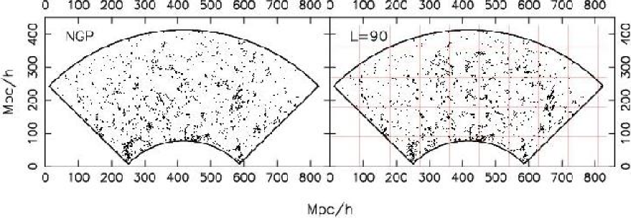
Table I summarizes some properties of all the subsamples which we have used in our analysis. The galaxy positions in all the subsamples were projected onto the equatorial plane to obtain the 2D galaxy distributions (Figure 1) which we have analyzed in the rest of the paper. A visual inspection of Figure 1 reveals the presence of large-scale coherent patterns namely the interconnected network of filaments and voids which we now proceed to quantify. For both the NGP and SGP subsamples (Table I), we have generated 9 random realizations (Figure 2) which contain exactly the same number of galaxies randomly distributed over the same volume as the actual data.

Table I
Sample Abs. Mag No. of galaxies NGP $-22.6\leq M_{r}\leq-21.6$ $3297$ NGP faint $-22.1\leq M_{r}\leq-21.6$ $2221$ NGP bright $-22.6\leq M_{r}<-22.1$ $1076$ NGP uniform thickness $-22.6\leq M_{r}\leq-21.6$ $1936$ SGP $-22.6\leq M_{r}\leq-21.6$ $2018$ SGP faint $-22.1\leq M_{r}\leq-21.6$ $1206$ SGP bright $-22.6\leq M_{r}<-22.1$ $812$ SGP uniform thickness $-22.6\leq M_{r}\leq-21.6$ $1096$

2.2 Method of Analysis

For each of the subsamples described in the previous subsection, the 2D galaxy distribution was embedded in a $1\,h^{-1}{\rm Mpc}\times 1\,h^{-1}{\rm Mpc}$ 2D rectangular grid. Grid cells having a galaxy within them are termed as filled and were assigned the value 1, whereas cells with no galaxy are termed as empty and were given the value 0. The grid cells which are beyond the boundaries of the survey were assigned a negative value in order to distinguish them from the empty cells within the survey area. The net result of is that the galaxy distribution is now represented through a distribution of 1s and 0s located on a 2D grid.

The next step is to use an objective criteria to identify the coherent large-scale structures visible in the galaxy distribution. We use a “friends-of-friends”(FOF) algorithm to identify interconnected regions of filled cells which we refer to as clusters. In this algorithm any two adjacent filled cells are referred to as friends. Clusters are defined through the stipulation that any friend of my friend is my friend. The distribution of 1s on the grid is very sparse with only $\sim 1\%$ of the cells being filled. Also, the filled cells are mostly isolated, and the clusters identified using FOF, which contain only a few cells each, do not correspond to the large-scale coherent structures seen in the SDSS strips. It is necessary to smoothen or coarse-grain the galaxy distribution so that the large scale structures may be objectively identified.

Figure 3: This shows the NGP and SGP strips at different levels of coarse-graining indicated by $N$ in the figure along with the corresponding filling factor $FF$. Only the large clusters are shown, different shades (colours) being used to demarcate individual clusters.

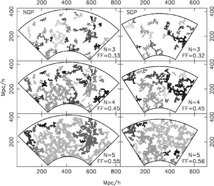
The coarse-graining is carried out by gradually making each filled cell fatter until the filled cells overlap and they finally fill up the whole survey area. In every iteration of coarse-graining we fill up all the empty cells which are adjacent to filled cells, causing every filled cell to grow fatter. This causes clusters to grow, first because of the growth of filled cells, and then by the merger of adjacent clusters as they overlap. This process is illustrated in Figure 3. At the initial stages of coarse-graining, the patterns which emerge from the distribution of 1s and 0s closely resembles the coherent structures seen in the galaxy distribution. As the coarse-graining proceeds, the clusters become very thick and fill up the entire region washing away any visibly distinct pattern. The filling factor ${\rm FF}$, defined as the fraction of cells within the survey area that are filled, ie.

$${\rm FF}=\frac{{\rm Total\,No.\,of\,Filled\,Cells}}{{\rm Total\,No.\,of\,Cells\,Inside\,the\,Survey\,Area}}$$ (1)

increases from ${\rm FF}\sim$ 0.01 to ${\rm FF}=$ 1 as the coarse graining proceeds. So as to not restrict our analysis to an arbitrarily chosen level of smoothing, we analyze the clusters identified in the pattern of 1s and 0s after each iteration of coarse-graining ie. the whole range of ${\rm FF}$.

2.2.1 LCS and Shapefinders

At each level of coarse-graining we identify the largest cluster and calculate the Largest Cluster Statistic (LCS) defined as the fraction of the filled cells in the largest cluster

$${\rm LCS}=\frac{{\rm No.\,of\,Filled\,Cells\,in\,the\,Largest\,Cluster}}{{\rm Total\,No.\,of\,Filled\,Cells}}\,.$$ (2)

We study the growth of LCS with increasing FF (Figures 5 and 6) to quantify the tendency of clusters to get interconnected as the coarse-graining proceeds (Figure 3). The transition from many small clusters to a network of interconnected filaments running across almost the entire survey, which is the onset of percolation, is manifested by a sharp increase in LCS.

The geometry and topology of a two dimensional cluster can be described by the three Minkowski functionals, namely its area $S$, perimeter $P$, and genus $G$. It is possible to quantify the shape of the cluster using a single 2D “Shapefinder” statistic (Bharadwaj et al. 2000) which is defined as the dimensionless ratio

$${\cal F}=\frac{P^{2}-4\pi S}{P^{2}+4\pi S}\,,$$ (3)

which by construction has values in the range $0\leq{\cal F}\leq 1$. It can be verified that ${\cal F}=1$ for an ideal filament which has a finite length and zero width, whereby it subtends no area ($S=0$) but has a finite perimeter ($P>0$). It can be further checked that ${\cal F}=0$ for a circular disk, and intermediate values of ${\cal F}$ quantifies the degree of filamentarity with the value increasing as a cluster is deformed from a circular disk to a thin filament.

The definition of ${\cal F}$ needs to be modified when working on a rectangular grid of spacing $l$. An ideal filament, represented on a grid, has the minimum possible width i.e. $l$, and its perimeter $P$ and area $S$ are related as $P=2S+2l$. At the other extreme we have $P^{2}=16S$ for a square shaped cluster on the grid. We introduce the 2D Shapefinder statistic

$${\cal F}=\frac{(P^{2}-16S)}{(P-4l)^{2}}$$ (4)

to quantify the shape of clusters on a grid. By definition 0$\leq{\cal F}\leq$ 1. ${\cal F}$ quantifies the degree of filamentarity of the cluster, with ${\cal F}$ = 1 indicating a filament and ${\cal F}$ = 0, a square, and ${\cal F}$ changes from $0$ to $1$ as a square is deformed to a filament.

The extent of filamentarity in a survey is mostly dominated by the morphology of the most massive members as a large cluster has a greater contribution to the overall texture of large-scale structure than an individual galaxy.We therefore want to give greater weight to larger objects and used the second moment of filamentarity as the indicator of average filamentarity. The average filamentarity $F_{2}$ is defined as the mean filamentarity of all the clusters in a slice weighted by the square of the area of each clusters

$$F_{2}={\sum_{i}{\cal S}_{i}^{2}{\cal F}_{i}\over\sum_{i}{\cal S}_{i}^{2}}\,.$$ (5)

In the current analysis, we study the average filamentarity $F_{2}$ as a function of FF (Figures 5 and 6) to quantify the degree of filamentarity in each of the SDSS subsamples and the random datasets.

2.2.2 Shuffle

We use a statistical technique called Shuffle to determine the largest length-scale at which the filamentarity is statistically significant. A grid with squares blocks of side $L$ is superposed on the original data slice (Figure 4). Blocks of data which lie entirely within the slice are then randomly interchanged, with rotation, repeatedly, to form a new shuffled slice. The shuffling process eliminates coherent features in the original data on scales larger than $L$, keeping clustering at scales below $L$ nearly identical to the original data. All the structures spanning length-scales greater than $L$ that exist in the shuffled slices are the result of chance alignments. At a fixed value of $L$, the average filamentarity in the original sample will be larger than in the shuffled data only if the actual data has more filaments spanning length-scales larger than $L$, than that expected from chance alignments. The largest value of $L$, $L_{\rm MAX}$, for which the average filamentarity of the shuffled slices is less than the average filamentarity of the actual data gives us the largest length-scale at which the filamentarity is statistically significant. Filaments spanning length-scales larger than $L_{\rm MAX}$ arise purely from chance alignments.

Figure 4: This figure exhibits how Shuffle works. The left panel shows the galaxy distribution in the NGP subsample and the right panel shows a shuffled realization generated from the same data using $L=90h^{-1}{\rm Mpc}$. A $90h^{-1}{\rm Mpc}\,\times\,90h^{-1}{\rm Mpc}$ grid was placed on the NGP data, and square blocks lying fully inside the survey region were randomly shuffled around to generate the data shown in the right panel. This process destroys all coherent structures spanning length-scales larger than $L=90h^{-1}{\rm Mpc}$ in the actual data and filaments larger than this in the shuffled data arise from chance alignments. Among the filaments seen in the right panel, those which run across the block boundaries have formed purely from chance alignments.

We have used the uniform thickness subsamples (Table I) which have thickness $8.2\,h^{-1}\,{\rm Mpc}$ for the Shuffle analysis. For each value of $L$ we generated $24$ different realization of the shuffled slices. To ensure that the edges of the blocks which are shuffled around do not cut the actual filamentary pattern at exactly the same place in all the realizations of the shuffled data, we randomly shifted the origin of the grid used to define the blocks. The values of FF and $F_{2}$ in the 24 realizations differ from one another and from the actual data at the same stage of coarse-graining. So as to be able to quantitatively compare the shuffled realizations with the actual data, we interpolate the values of $F_{2}$ in the shuffled realization at the values of FF obtained for the actual data. The mean $\bar{F_{2}}[{\rm Shuffled}]$ and the variance $(\Delta F_{2}[{\rm Shuffled}])^{2}$ of the average filamentarity was determined for the shuffled data at each value of FF using the 24 realizations. The difference between the filamentarity of the shuffled data and the actual data was quantified using the reduced $\chi^{2}$ per degree of freedom

$$\frac{\chi^{2}}{\nu}=\frac{1}{N_{p}}\sum_{a=1}^{N_{p}}\frac{(F_{2}[{\rm Actual}]-\bar{F_{2}}[{\rm Shuffled}]))_{a}^{2}}{(\Delta F_{2}[{\rm Shuffled}])_{a}^{2}}$$ (6)

where the sum is over different values of the filling factor FF.

3 Results

3.1 Comparison with random samples

Figure 5 shows the results for the NGP and SGP strips plotted along with the values for their random counterparts. For both NGP and SGP we have 9 random realizations which were analyzed in exactly the same way as the actual data. The values of the filling factor FF differ from realization to realization at the same level of coarse-graining, and we interpolated the values of LCS and $F_{2}$ at the values of FF obtained for the actual data, and these were used to obtain the mean and the $1-\sigma$ error-bars shown for the random data in the figure. It may be noted that the values of LCS and $F_{2}$ show very little variation from realization to realization, and this is reflected in the very small error-bars. This is a consequence of the high number density and large area of the two SDSS strips analyzed here.

For both the actual data and the random realizations, the LCS, has a very small value at low values of FF. For the actual data, LCS is below $0.2$ up to a filling factor of $0.4$ ie. the largest cluster contains less than $20\%$ of the filled cells when around $40\%$ of the cells in the survey area are filled. A transition is seen to occur at FF in the range $0.5-0.6$ for both the NGP and SGP strips, and the largest cluster contains more than $80\%$ of all the filled cells at a filling factor ${\rm FF}=0.65$. This sharp transition from a set of small clusters at ${\rm FF}<0.4$ to a single large cluster which is a network of filaments running across almost the entire survey is referred to as the percolation transition and it is found to occur at a threshold value of the filling factor around ${\rm FF}=0.5$. The LCS of the random data is less than that of the actual data for nearly the entire range of FF, the two curves being many factors of $\sigma$ apart. Also, in the random data ${\rm LCS}<0.2$ all the way to ${\rm FF}=0.5$ whence it exhibits a sudden rise to ${\rm LCS}=0.7$ at ${\rm FF}=0.65$. The faster growth of LCS with increasing FF in the two SDSS strips as compared to the random Poisson point distribution, and the onset of percolation at a lower value of FF in the actual data show the presence of network like topology in the galaxy distribution.

Turning our attention next to the average filamentarity $F_{2}$, we find that initially $F_{2}$ is larger in the actual data as compared to the random data. For both the actual and the random data $F_{2}$ increases with successive iterations of coarse-graining and reaches a value $F_{2}\sim 1$ at ${\rm FF}=0.6$. This corresponds to a situation where nearly all the clusters have merged into a single cluster (${\rm LCS}\sim 0.8$) and further smoothing results in only fattening this cluster causing the average filamentarity to fall. The region beyond ${\rm FF}=0.6$ is not of importance and is not considered in our analysis. The average filamentarity of the actual data is larger than that for a Poisson point distribution for the entire range of filling factor ${\rm FF}\leq 0.6$. This shows that the two SDSS strips analyzed here are largely dominated by filaments, significantly in excess of that expected in a random distribution of points.

Figure 5: This shows the Largest Cluster Statistics (LCS) and the Average Filamentarity ($F_{2}$) for two of the SDSS strips together with the values for their random counterparts. We have used 9 realizations to determine the mean values and the $1-\sigma$ error-bars shown for the random data.

3.2 Luminosity Dependence

The bright and faint subsamples were separately analyzed to investigate the luminosity dependence, if any, of the connectivity and the shapes of the patterns in the galaxy distribution. For both the SGP and the NGP the subsample of faint galaxies (Table I) contains roughly $1.5$ to $2$ times the number of galaxies in the subsample of bright galaxies distributed over the same region. So as to compare the bright and faint subsamples at the same galaxy number density we randomly extracted a subset of the faint subsamples so that the number exactly matches the bright subsamples. Five such randomly chosen subsets were used to make bootstrap estimates of the mean and the $1-\sigma$ fluctuations of LCS and $F_{2}$ as function of ${\rm FF}$ (Figure 6). These were compared with LCS and $F_{2}$ for the bright subsample to test if there is any statistically significant evidence for a luminosity dependence.

We find that the values of both LCS and $F_{2}$ are larger for the faint subsamples as compared to the bright ones. The percolation transition occurs at a smaller value of $FF$ for the faint subsamples, indicating that a network like topology is more dominant in the distribution of faint galaxies as compared to the bright ones. Also, the faint galaxies have a more filamentary distribution, quantified by $F_{2}$, as compared to the bright galaxies. Using the reduced $\chi^{2}$ per degree of freedom to asses the statistical significance of these differences we find that $\chi^{2}/\nu=(72,39)$ in NGP and SGP respectively for the Largest Cluster Statistics and $(16,97)$ for the Average Filamentarity. This establishes that the luminosity dependence is a statistically significant effect.

Figure 6: The average filamentarity and largest cluster statistics vs. filling factor for bright and faint galaxies in the volume limited samples.The $1-\sigma$ error-bars for faint galaxies are shown in the figure.

Figure 7: This shows the Average Filamentarity for the two SDSS slices together with the results for the shuffled data for three values of $L$ shown in the figure. Shuffling with $L=20h^{-1}\,{\rm Mpc}$ causes a large drop in the Average Filamentarity showing the statistical significance of the filamentarity at this length-scale. The filamentarity is statistically significant up to $L_{MAX}=80h^{-1}\,{\rm Mpc}$ where the actual data lies above the the $1-\sigma$ error-bars. The data is within the $1-\sigma$ error-bars of the shuffled realizations for larger values of $L$, indicating that the filaments are not statistically significant beyond $L_{MAX}$. The data point for $L=80h^{-1}\,{\rm Mpc}$ have been slightly shifted to prevent the error-bars from overlapping in the figure.

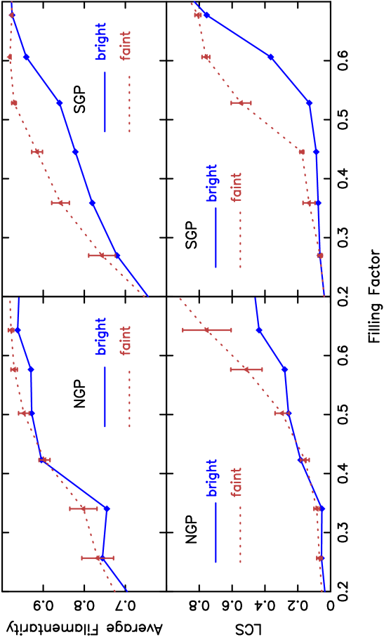
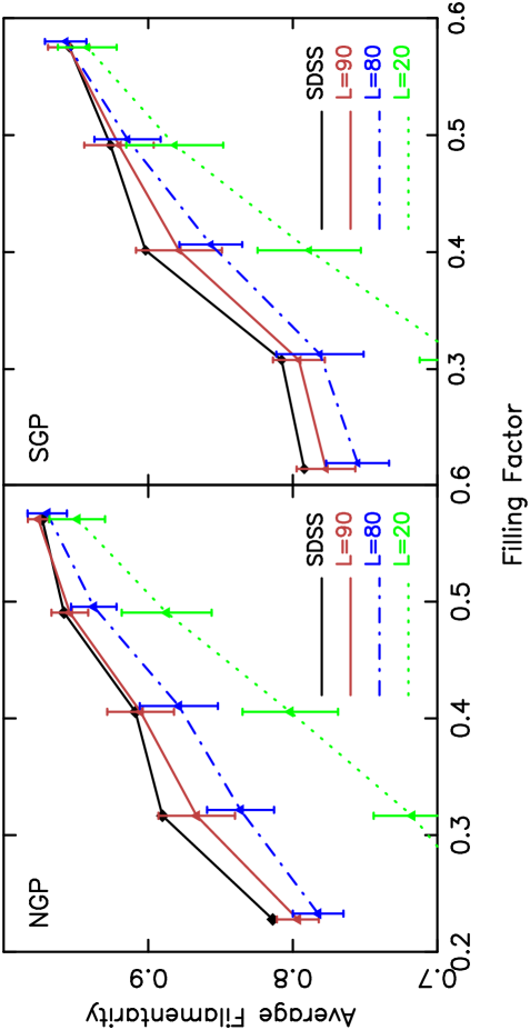
Table II
L $\chi^{2}/\nu$(NGP) $\chi^{2}/\nu$(SGP) 20 16.64 15.1 30 11.7 5.2 40 5.8 4.53 50 5.3 1.64 60 3.43 2.85 70 2.2 1.8 80 2.33 1.65 90 1.08 0.82 100 0.58 0.46 110 1.03 0.66 120 1.13 0.33 130 0.5 0.5 140 0.5 0.4 150 0.4 0.3

Figure 8: This shows the $\chi^{2}/\nu$ at different shuffling lengths $L$ for both the NGP and SGP slices.

3.3 Statistical Significance of the Filaments

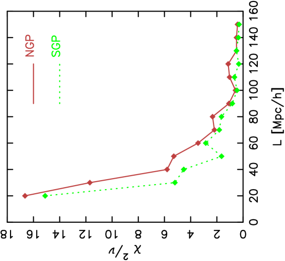
We applied Shuffle to the NGP and the SGP uniform thickness subsamples varying $L$ from $20$ to $150\,h^{-1}\,{\rm Mpc}$ in steps of $10\,h^{-1}\,{\rm Mpc}$. The Average Filamentarity falls substantially if the data is Shuffled using $L\,=\,20\,h^{-1}\,{\rm Mpc}$ (Figure 7) indicating that a large fraction of the filaments are cut by the Shuffling mechanism and the number of filaments which are produced by chance alignments in the Shuffled data are less than the number of filaments destroyed. This establishes that the filaments do not arise from chance alignments and are statistically significant, genuine features of the galaxy distribution at this length-scale.

Longer filaments survive the Shuffling process as $L$ is increased and hence the Average Filamentarity increases with $L$ , slowly approaching the values for the actual data. The values of $\chi^{2}/\nu$ given in Table II and shown graphically in Figure 8 quantify the difference in $F_{2}$ between the Shuffled and the actual data. We find that Shuffling the data with $L=90\,h^{-1}\,{\rm Mpc}$ or larger doesn’t result in a statistically significant drop in $F_{2}$, the value of $\chi^{2}/\nu$ being $\sim 1$ for $L\geq 90\,h^{-1}\,{\rm Mpc}$. The value of $L_{MAX}$, the largest length-scale at which Shuffling causes $F_{2}$ to fall, is $80\,h^{-1}\,{\rm Mpc}$ for both NGP and SGP. This is the largest length-scale at which the filaments are statistically significant.

Cutting the galaxy distribution into blocks of size $90\,h^{-1}\,{\rm Mpc}$ or larger and shuffling them around does not reduce the Average Filamentarity. Filaments spanning length-scales larger than $90\,h^{-1}{\rm Mpc}$ are present in equal abundance in the Shuffled and the actual data showing that these filaments arise purely from chance alignments.

The Average Filamentarity for $L=80\,h^{-1}{\rm Mpc}$ and $90\,h^{-1}{\rm Mpc}$ where we have the transition from statistically significant filaments to filaments that arise purely from chance is shown in Figure 7 along with the actual data. It may be noted that we have restricted our analysis to $0.2\leq{\rm FF}\leq 0.6$ as there are many small clusters which bear no resemblance to the filaments we wish to characterize for ${\rm FF}<0.2$ and nearly all the filaments get interconnected into a single dominant cluster for ${\rm FF}>0.6$.

4 Discussion and Conclusion

The large-scale network of filaments and voids is one of the most striking visual features in all galaxy redshift surveys e.g., CfA(Geller & Huchra 1989), LCRS (Shectman et al., 1996), 2dFGRS(Colles et al. 2001) and SDSS(EDR) (Stoughton et al. 2002, Abazajian et al. 2003). The SDSS, the largest redshift survey to date, offers a unique opportunity to study these features at a high level of precisions on hitherto unprecedented length-scales. We have used the Largest Cluster Statistics (LCS) and the Average Filamentarity ($F_{2}$) to study respectively the interconnectivity and the shapes of the patterns seen in the galaxy distribution in 2D projections of volume limited subsamples from the two equatorial strips in the SDSS DR1. These were studied as functions of the Filling Factor (FF) at different levels of smoothing, and the results compared to a 2D Poisson point distribution. We find that at the same value of FF, the values of LCS and $F_{2}$ in both the NGP and the SGP strips are substantially larger than those of the random distributions for nearly the entire range of FF. This indicates a high level of connectivity consistent with a network like topology with filaments being the dominant structures in the galaxy distribution. Individual filamentary structures identified at low filling factors $({\rm FF}\sim 0.3)$ get interconnected into a network at the percolation transition $({\rm FF}\sim 0.5-0.6)$.

The high number density of galaxies in the SDSS allows us to test if there is evidence for luminosity dependence in the connectivity and the filamentarity. We find that the distribution of the brighter galaxies exhibits lesser connectivity and filamentarity compared to the fainter galaxies in the same region. This is consistent with the picture where the brighter galaxies preferentially reside in the compact high density regions whereas the fainter galaxies have a more diffuse distribution. Studies using N-body simulations (Bharadwaj & Pandey, 2004) have shown that the filamentarity is highly sensitive to bias, with the large-scale filamentarity falling with increasing bias. The findings of this paper reaffirm that the brighter galaxies have a higher bias relative to the fainter ones as noted from earlier studies of the luminosity dependence of the galaxy clustering (eg. Norberg et al. 2001, Zehavi et al. 2002). Einasto et al. (2003) have studied the luminosity distribution of galaxies in high and low density regions of the SDSS to show that the brighter galaxies are preferentially distributed in high density environments. Goto et al. (2003) have studied the morphology-density relation in the SDSS(EDR) and find that this relation is less noticeable in the sparsest regions indicating requirment of denser environment for the physical mechanisms responsible for galaxy morphological change. Studies of the connectivity using the genus statistics (Hoyle et al., 2002) have revealed colour dependence with the redder galaxies showing a lesser connectivity compared to the blue ones. Hogg et al. (2003) and Blanton et al. (2003b) find a strong environment dependence for both the colour and luminosity for the SDSS galaxies. Their results indicate that the red galaxies are found preferentially in overdense regions relative to the blue galaxies. These observations showing the connectivity and filamentarity to depend on the luminosity and the color of the galaxies poses interesting questions about both, the models of galaxy formation and our understanding of the formation of the filament-void network. It may be noted that the colour dependence of the filamentarity has not been studied here and it is proposed to take this up in the future.

Studies of the genus statistics at large values of smoothing shows the SDSS to be consistent with a Gaussian random field Hoyle et al. (2002). Our analysis of the connectivity starting with the unsmoothed data and analyzing it at various levels of smoothing complements the earlier analysis and reveals the presence of strongly non-Gaussian features, namely the filaments. It is interesting to note that these filaments are the natural outcome of gravitational instability starting from Gaussian random initial conditions.

We have determined the largest length-scale at which the filaments are statistically significant. We find that filaments spanning length-scales up to $80\,h^{-1}\,{\rm Mpc}$ are statistically significant in both the SDSS strips we have analyzed. Filaments spanning scales larger than this are the outcome of purely chance alignments in the galaxy distribution. The analysis presented here has distinct advantages over the earlier analysis using the LCRS (Bharadwaj et al., 2004). The SDSS strips are substantially larger than the LCRS, and hence there are more blocks which can be shuffled around giving us better statistics for the results. Further, the LCRS wedges were curved and had varying thickness whereas our SDSS subsamples are flat and have uniform thickness. Our results are consistent with the earlier findings for the LCRS where filamentarity was found to be statistically significant on scales up to $70-80\,h^{-1}\,{\rm Mpc}$ in the $-3^{\circ}$ slice and $50-70\,h^{-1}\,{\rm Mpc}$ in the other 5 slices. It is interesting to note that the results of the analysis of mock SDSS catalogues based on $\Lambda{\rm CDM}\,\,$N-body simulations (Sheth, 2004) reveal the length of the longest superclusters to be $\sim 60\,h^{-1}\,{\rm Mpc}$. A similar analysis of the supercluster-void network in VIRGO $\Lambda{\rm CDM}\,\,$N-body simulations show the most massive superclusters to exceed $50\,h^{-1}\,{\rm Mpc}$ in length. It may be noted that our analysis gives an upper limit to the linear length-scale up to which the filaments are statistically significant. The individual filaments may be wiggly or coiled up, and the length measured along the filament may be larger.

The connectivity and filamentarity of the two SDSS strips are roughly consistent with each other, though we have not performed a quantitative comparison given the different geometries of the two subsamples. It may be noted that the filaments identified in our 2D analysis may actually be the intersection of 3D planar structures. Analysis of the SDSS power-spectrum (Tegmark et al., 2004a) shows the presence of a bump at the Fourier mode $k\sim 0.05\,h\,{\rm Mpc}^{-1}$ in the power spectrum. While it may be speculated that the high level of filamentarity detected in the SDSS may be a consequence of this features, earlier analysis using N-body simulations show the filamentarity to be insensitive to the presence of such a bump (Bharadwaj & Pandey, 2004).

In conclusion we note that our results confirm the earlier results (Bharadwaj et al., 2004) that the filaments seen in the galaxy distribution are the largest known statistically significant structures in the universe.

5 Acknowledgment

SB would like to acknowledge financial support from the Govt. of India, Department of Science and Technology (SP/S2/K-05/2001). BP would like to thank the CSIR, Govt. of India for financial support through a JRF fellowship. The authors would like to thank Scot Kleinman, Michael Blanton and Sebastian Jester for help in accessing and understanding the SDSS data. The SDSS DR1 data was downloaded from the SDSS skyserver http://skyserver.sdss.org/dr1/en/.

Funding for the creation and distribution of the SDSS Archive has been provided by the Alfred P. Sloan Foundation, the Participating Institutions, the National Aeronautics and Space Administration, the National Science Foundation, the U.S. Department of Energy, the Japanese Monbukagakusho, and the Max Planck Society. The SDSS Web site is http://www.sdss.org/.

The SDSS is managed by the Astrophysical Research Consortium (ARC) for the Participating Institutions. The Participating Institutions are The University of Chicago, Fermilab, the Institute for Advanced Study, the Japan Participation Group, The Johns Hopkins University, the Korean Scientist Group, Los Alamos National Laboratory, the Max-Planck-Institute for Astronomy (MPIA), the Max-Planck-Institute for Astrophysics (MPA), New Mexico State University, University of Pittsburgh, Princeton University, the United States Naval Observatory, and the University of Washington.

References

- Abazajian et al. (2003) Abazajian, K., et al. 2003, AJ, 126, 2081
- Abazajian et al. (2004) Abazajian, K., et al. 2004, AJ, 128, 502
- Basilakos, Plionis, & Rowan-Robinson (2001) Basilakos, S., Plionis, M., & Rowan-Robinson, M. 2001, MNRAS, 323, 47
- Bharadwaj et al. (2000) Bharadwaj, S., Sahni, V., Sathyaprakash, B. S., Shandarin, S. F., & Yess, C. 2000, ApJ, 528, 21
- Bharadwaj et al. (2004) Bharadwaj, S., Bhavsar, S. P., & Sheth, J. V. 2004, ApJ, 606, 25
- Bharadwaj & Pandey (2004) Bharadwaj, S., Pandey, B. 2004, ApJ,Accepted, astro-ph/0405059
- Bhavsar & Ling (1988) Bhavsar, S. P. & Ling, E. N. 1988, ApJL, 331, L63
- Blanton et al. (2003a) Blanton, M. R., Lin, H., Lupton, R. H., Maley, F. M., Young, N., Zehavi, I., & Loveday, J. 2003, AJ, 125, 2276
- Blanton et al. (2003b) Blanton, M. R., et al. 2003, ApJ, 594, 186
- Connolly et al. (2002) Connolly, A. J., et al. 2002, ApJ, 579, 42
- Colles et al. (2001) Colles, M. et al.(for 2dFGRS team) 2001,MNRAS,328,1039
- Doroshkevich et al. (2004) Doroshkevich, A., Tucker, D. L., Allam, S.,& Way, M. J. 2004, A&A, 418,7
- Dodelson et al. (2002) Dodelson, S., et al. 2002, ApJ, 572, 140
- Einasto et al. (1984) Einasto, J., Klypin, A. A., Saar, E., & Shandarin, S. F. 1984, MNRAS, 206, 529
- Einasto et al. (2003) Einasto, J., Hütsi, G., Einasto, M., Saar, E., Tucker, D. L., Müller, V., Heinämäki, P., & Allam, S. S. 2003, A&A, 405, 425
- Eisenstein et al. (2001) Eisenstein, D. J., et al. 2001, AJ, 122, 2267
- Fukugita et al. (1996) Fukugita, M., Ichikawa, T., Gunn, J. E., Doi, M., Shimasaku, K., & Schneider, D. P. 1996, AJ, 111, 1748
- Gunn et al. (1998) Gunn, J. E., et al. 1998, AJ, 116, 3040
- Gott, Dickinson, & Melott (1986) Gott, J. R., Dickinson, M., & Melott, A. L. 1986, ApJ, 306, 341
- Goto et al. (2003) Goto, T., Yamauchi, C., Fujita, Y., Okamura, S., Sekiguchi, M., Smail, I., Bernardi, M., & Gomez, P. L. 2003, MNRAS, 346, 601
- Geller & Huchra (1989) Geller, M.J. & Huchra, J.P.1989, Science,246,897
- Hikage et al. (2003) Hikage, C., et al. 2003, Publications of the Astronomical Society of Japan, 55, 911
- Hogg et al. (2001) Hogg, D. W., Finkbeiner, D. P., Schlegel, D. J., & Gunn, J. E. 2001, AJ, 122, 2129
- Hogg et al. (2003) Hogg, D. W., et al. 2003, ApJL, 585, L5
- Hoyle et al. (2002) Hoyle, F., et al. 2002, ApJ, 580, 663
- Hoyle, Vogeley, & Gott (2002) Hoyle, F., Vogeley, M. S., & Gott, J. R. I. 2002, ApJ, 570, 44
- Infante et al. (2002) Infante, L., et al. 2002, ApJ, 567, 155
- Pimbblet, Drinkwater, & Hawkrigg (2004) Pimbblet, K. A., Drinkwater, M. J., & Hawkrigg, M. C. 2004, MNRAS, 354, L61
- Kolokotronis, Basilakos, & Plionis (2002) Kolokotronis, V., Basilakos, S., & Plionis, M. 2002, MNRAS, 331, 1020
- Lupton et al. (2002) Lupton, R. H., Ivezic, Z., Gunn, J. E., Knapp, G., Strauss, M. A., & Yasuda, N. 2002, Proceedings of the SPIE, 4836, 350
- Mecke, Buchert, & Wagner (1994) Mecke, K. R., Buchert, T., & Wagner, H. 1994, A&A, 288, 697
- Norberg et al. (2001) Norberg, P., et al. 2001, MNRAS, 328, 64
- Pier et al. (2003) Pier, J. R., Munn, J. A., Hindsley, R. B., Hennessy, G. S., Kent, S. M., Lupton, R. H., & Ivezić, Ž. 2003, AJ, 125, 1559
- Sahni, Sathyaprakash, & Shandarin (1998) Sahni, V., Sathyaprakash, B. S., & Shandarin, S. F. 1998, ApJL, 495, L5
- Sheth et al. (2003) Sheth, J. V., Sahni, V., Shandarin, S. F., & Sathyaprakash, B. S. 2003, MNRAS, 343, 22
- Sheth (2004) Sheth,J.V., 2004, MNRAS, 354, 332
- Shandarin & Zeldovich (1983) Shandarin, S. F. & Zeldovich, I. B. 1983, Comments on Astrophysics, 10, 33
- Shandarin & Yess (1998) Shandarin, S. F. & Yess, C. 1998, ApJ, 505, 12
- Shandarin, Sheth, & Sahni (2004) Shandarin, S. F., Sheth, J. V., & Sahni, V. 2004, MNRAS, 353, 162
- Shectman et al. (1996) Shectman, S. A.,Landy, S. D., Oemler, A., Tucker, D. L., Lin, H., Kirshner, R. P., & Schechter, P. L. 1996, ApJ, 470, 172
- Smith et al. (2002) Smith, J. A., et al. 2002, AJ, 123, 2121
- Stoughton et al. (2002) Stoughton, C., et al. 2002, AJ, 123, 485
- Strauss et al. (2002) Strauss, M. A., et al. 2002, AJ, 124, 1810
- Schmalzing & Buchert (1997) Schmalzing, J. & Buchert, T. 1997, ApJL, 482, L1
- Szapudi et al. (2002) Szapudi, I., et al. 2002, ApJ, 570, 75
- Szalay et al. (2002) Szalay, A. S., et al. 2002, Bulletin of the American Astronomical Society, 34, 777
- Tegmark et al. (2002) Tegmark, M., et al. 2002, ApJ, 571, 191
- Tegmark et al. (2004a) Tegmark, M., et al. 2004, ApJ, 606, 702
- York et al. (2000) York, D. G., et al. 2000, AJ, 120, 1579
- Zehavi et al. (2002) Zehavi, I., et al. 2002, ApJ,571,172