Globular Clusters with Dark Matter Halos. II. Evolution in Tidal Field

Abstract

In this second paper in our series, we continue to test primordial scenarios of globular cluster formation which predict that globular clusters formed in the early universe in the potential of dark matter minihalos. In this paper we use high-resolution $N$-body simulations to model tidal stripping experienced by primordial dark-matter dominated globular clusters in the static gravitational potential of the host dwarf galaxy. We test both cuspy Navarro-Frenk-White (NFW) and flat-core Burkert models of dark matter halos. Our primordial globular cluster with an NFW dark matter halo survives severe tidal stripping, and after 10 orbits is still dominated by dark matter in its outskirts. Our cluster with Burkert dark matter halo loses almost all its dark matter to tidal stripping, and starts losing stars at the end of our simulations. The results of this paper reinforce our conclusion in Paper I that current observations of globular clusters are consistent with the primordial picture of globular cluster formation.

1. INTRODUCTION

The primordial scenario of globular cluster (GC) formation was first proposed by Peebles & Dicke (1968). Their paper considers GCs forming in the early universe out of primordial gas fluctuations on a Jeans mass scale. Realization that the dominant mass component of the universe is dark matter (DM) led to the revision of this idea in Peebles (1984), where GCs are proposed to have formed in the potential wells of DM minihalos in the early universe. In this revised picture GCs can be considered as some of the earliest galaxies in the universe, with a baryons dominated core and extended DM halo. This picture of DM-dominated GCs forming in the early universe was later considered by many authors, including Rosenblatt, Faber, & Blumenthal (1988), Padoan, Jimenez, & Jones (1997), Cen (2001), Bromm & Clarke (2002), and Beasley et al. (2003).

Primordial GCs could have formed somewhere between a redshift of $\sim 30$, when the first stars in the universe are believed to have been born inside minihalos with total masses $10^{5}-10^{6}$ $M_{\odot}$ (Yoshida et al., 2003), and redshift of $\sim 6$, when the reionization of the universe was complete (Becker et al., 2001). It is often assumed that the very first stellar objects produced enough Lyman-Werner photons (capable of dissolving H₂ molecules, which are the main coolant in the pristine gas) to prohibit star formation in most of the low mass ($\lesssim 10^{8}$ $M_{\odot}$) gas-rich halos. Cosmological simulations with radiative transfer of Ricotti, Gnedin, & Shull (2002) suggest another possibility: in their model, numerous mini-galaxies with masses of $\lesssim 10^{8}$ $M_{\odot}$ form inside relic cosmological H ii regions. The observed positive feedback can be explained by high non-equilibrium fraction of free electrons in defunct H ii regions, which leads to enhanced H₂ production and hence star formation. This is an interesting mechanism for forming GCs, as it naturally explains the observed higher specific frequency of GCs in higher density regions of the universe (such as around cD galaxies at the center of clusters of galaxies), where large cosmological H ii regions should have formed in the early universe.

In a widely accepted hierarchical paradigm of structure formation in the universe, small bound objects form first, later merging to form objects of increasingly larger size. In this picture, primordial GCs would first experience a major merger with comparable mass halos, or be accreted by a larger halo of a dwarf galaxy size. In their simulations of the formation of a dwarf galaxy in the early universe (at $z\gtrsim 10$), Bromm & Clarke (2002) observed a formation of GC-type baryonic objects inside DM minihalos, which later merged to form a dwarf galaxy. By the end of the simulations, baryonic cores, believed to represent proto-GCs, had apparently lost their individual DM halos. Bromm & Clarke (2002) suggested that DM was lost because of the violent relaxation accompanying the major merger. The lack of resolution did not allow the authors to reach more definitive conclusion as to the fate of DM in their proto-GCs.

In the next step, dwarf galaxies containing primordial GCs would merge to produce objects of increasingly larger size. This process should continue at the present time. A well-known example is that of Sagittarius dwarf galaxy, which is presently in the process of being disrupted by the tidal forces of Milky Way and depositing its system of GCs into the halo of our Galaxy (Bellazzini, Ferraro, & Ibata, 2003).

In the primordial picture of GC formation, GCs can be considered as small nucleated dwarfs accreted at some point by larger galaxies, which lose their extra-nuclear material (baryons and DM) due to stripping by the tidal forces of the accreting galaxy. Such mechanism was invoked to explain the formation of a few of the largest GCs: M51 (Layden & Sarajedini, 2000), $\omega$ Centauri (Tsuchiya, Dinescu, & Korchagin, 2003; Mizutani, Chiba, & Sakamoto, 2003), and G1 (Bekki & Chiba, 2004), which is the satellite of the M31 galaxy. In the quoted papers, these GCs are considered to be exceptions. We suggest instead that this method of forming these GCs is a rule rather than exception, and is fully consistent with primordial GC formation scenarios. In this picture, the above largest GCs are examples of the most recent GC-producing accretion events, and represent a small fraction of the total number of proto-GCs accreted directly by a large galaxy (Milky Way or M31) in the modern universe (thus skipping the intermediate step of being accreted by a larger dwarf galaxy in the early universe).

Moore (1996) used numerical simulations of a DM-dominated GC orbiting inside the static potential of Milky Way halo and observations of tidal tails of M2 of Grillmair et al. (1995) to claim that primordial scenarios of GC formation are inconsistent with observations of Galactic GCs. As discussed by Bromm & Clarke (2002) and Beasley et al. (2003), the model of Moore was too simplistic to address this issue. Most importantly, the author considered all Galactic GCs being directly accreted by the Milky Way, which is definitely not the case in the hierarchical picture of structure formation in the universe. Moreover, the DM subhalo model of Moore (1996) is a lowered isothermal sphere with arbitrary (not cosmologically normalized) structural parameters, which makes it very different from the DM halos expected to host a GC in the early universe.

One also has to be careful with claims on the existence of “extratidal features” around Galactic satellites, which includes both GCs and dwarf spheroidal galaxies. In the case of $\omega$ Centauri, Law et al. (2003) showed that the apparent “tidal tails” observed by Leon, Meylan, & Combes (2000) around this GC are most probably caused by spatially variable foreground dust extinction in its outskirts. In the case of the Draco dwarf spheroidal galaxy, the detection of apparent “extratidal features” around this galaxy by Irwin & Hatzidimitriou (1995) was later refuted by observations of Odenkirchen et al. (2001) which had much higher sensitivity. The “extratidal” extension of the radial surface brightness profiles of Galactic GCs beyond a “tidal” King radius is almost always seen at the levels lower than the inferred background contamination level, and could be an artifact of the background correction procedure. One beautiful example of a GC with obvious tidal tails is that of Palomar 5 (Odenkirchen et al., 2003). As we will show in this paper, a presence of tidal tails in some GCs is not inconsistent with these GCs having formed with DM halos in the early universe, and hence with primordial scenarios of GC formation.

In this series of two papers, we are using high-resolution $N$-body simulations of GCs with DM halos to test primordial scenarios of GC formation. In particular, we are trying to answer the following questions: 1) Are there obvious signatures of DM presence in GCs? 2) Will DM in a primordial GC survive hierarchical process of assembling galaxies in the early universe? In the first paper, Mashchenko & Sills (2004b, hereafter Paper I), we considered the initial relaxation of a stellar cluster at the center of a DM minihalo in the early universe (around $z=7$). The structural parameters of DM halos were fixed by results of cosmological $\Lambda$CDM simulations. The initial non-equilibrium configuration of stellar clusters was that of Mashchenko & Sills (2004a, hereafter MS04), where we showed that purely stellar (no DM) homogeneous isothermal spheres with the universal values of the initial density $\rho_{i,*}=14$ $M_{\odot}$ pc^-3 and velocity dispersion $\sigma_{i,*}=1.91$ km s^-1 collapse to form GC-like clusters, with all bivariate correlations between structural and dynamic parameters of Galactic GCs being accurately reproduced. We showed in Paper I that many observational features of Galactic GCs, used traditionally to argue that these systems are tidally limited purely stellar clusters without DM, can be produced by the presence of significant amounts of DM in their outskirts. In particular, in warm collapse models (with the initial virial parameter for the stellar core of $0.27\lesssim\nu\lesssim 1.7$) we observed the formation of an apparent “tidal” cutoff in surface brightness profiles, with no unusual features in the outer parts of the velocity dispersion profile. In cold collapse models (with $\nu\lesssim 0.27$), on the contrary, an apparent “break” in the outer parts of both surface brightness and velocity dispersion profiles is seen, which can be mistakingly interpreted as presence of “extratidal” stars heated by the tidal field of the host galaxy.

The results of Paper I are directly applicable to dynamically young intergalactic GCs and GCs which have not experienced significant tidal stripping in the potential of the host galaxies. In this second paper, we test the regime of severe tidal stripping of our primordial DM-dominated GCs in the potential of the host dwarf galaxy. As we discussed above, being accreted by a dwarf galaxy would be a typical fate of primordial GCs formed at high redshift. We use warm collapse models of primordial GCs from Paper I to set up the initial conditions for the present paper. We consider both simulations suggested Navarro, Frenk, & White (1997, hereafter NFW) and observationally motivated Burkert (1995) density profiles for our DM halos.

This paper is organized as follows. In Section 2 we describe our models. In Section 3 we discuss the results of the simulations. We conclude with Section 4.

2. MODEL

2.1. Physical Parameters of the Models

In our model, we explore the impact of tidal fields on DM-dominated GCs orbiting inside a static potential of host dwarf galaxy with a virial mass of $10^{9}$ $M_{\odot}$. GCs are assumed to be accreted by the dwarf galaxy at a redshift of $z=3$. Structural parameters (virial radius $R_{\rm vir}$, scale radius $R_{s}$, and concentration $C\equiv R_{\rm vir}/R_{s}$) of the host galaxy are fixed by the results of cosmological $\Lambda$CDM simulations, and at $z=3$ are equal to $R_{\rm vir}=8.16$ kpc, $R_{s}=1.21$ kpc, and $C=6.75$ (see eqs. [1-9] from Paper I). Throughout this paper we assume the following values of the cosmological parameters: $\Omega_{m}=0.27$ and $H=71$ km s^-1 Mpc^-1 (Spergel et al., 2003). Galaxies with $M_{\rm vir}=10^{9}$ $M_{\odot}$ correspond to $\sim 1\sigma$ density fluctuations collapsing at $z=3$ (Barkana & Loeb, 2001, their Fig. 6) and hence are very common at that redshift.

The initial parameters of our GCs are identical to those of our warm collapse models from Paper I. We could not use the cold collapse model of Paper I because it would be an impossible task with the present day technology with the method we are using ($N$-body simulations). Indeed, all the models presented in the present paper for the warm collapse only case required 3.6 CPU-years to run. The cold collapse models from Paper I (models C_n,b) took $\sim 7$ times longer to run than the warm collapse ones (models W_n,b) for the same evolution time, which is mainly due to $\sim 6$ times shorter stellar crossing time in the cold models. In addition, to run the cold collapse models of Paper I for the much longer evolution time of the present paper (3 Gyr), we would have to increase significantly the accuracy of the integration, and increase the number of DM particles by a factor of 20 (up to $10^{7}$ particles) to avoid artificial mass segregation effects which should be very significant for such long evolution time. As a result, the time required to simulate the cold collapse models for 3 Gyr would be two or more orders of magnitude longer than for the warm collapse case, or a few hundred CPU-years, which is obviously not feasible. The reasons for choosing the warm versus hot collapse model are that the warm one corresponds to a more typical GC (with the mass of $\sim 10^{5}$ M_⊙ for the warm model versus $\sim 10^{4}$ M_⊙ for the hot one), and that the warm model of Paper I exhibits interesting tidal-like features in the outskirts of the cluster (namely, a cutoff in the surface brightness profile) caused by the presence of DM halo, whereas the hot collapse model does not have any such features.

An isothermal homogeneous stellar sphere with the universal values of the initial stellar density and velocity dispersion, $\rho_{i,*}=14$ $M_{\odot}$ pc^-3 and $\sigma_{i,*}=1.91$ km s^-1 (MS04), is set at the center of a DM halo with either NFW or Burkert density profiles. The virial mass of the DM halo is $m_{\rm DM}=10^{7}$ $M_{\odot}$. The stellar mass is $m_{*}=8.8\times 10^{4}$ $M_{\odot}$, so the baryonic-to-DM mass ratio is $\chi=0.0088$. Our fiducial value of $\chi$, on one hand, is larger than the fraction of baryons in GCs of $\simeq 0.0025$ (McLaughlin, 1999), and on the other hand, is smaller than the universal baryonic-to-DM density ratio of $\simeq 0.20$ (Spergel et al., 2003). We assumed GCs have formed at $z=7$, so the structural parameters of their DM halos are $r_{\rm vir}=885$ pc, $r_{s}=181$ pc, and $c=4.88$ (from eqs. [1-9] of Paper I).

The initial virial ratio for our stellar clusters is $\nu_{*}=0.54$. The initial stellar radius is 11.2 pc. As we showed in Paper I, in the absence of DM our stellar cluster will first collapse (with the smallest value of the half-mass radius of $r_{*,\rm min}=3.0$ pc), and then bounce to form a relaxed cluster with a flat core, with the radius of $r_{0}=3.0$ pc, and a steep power-law outer density profile. The crossing time at the half-mass radius of the relaxed cluster is $\tau_{*}=0.49$ Myr. The crossing times at the half-mass radius for our DM halos are 52 and 61 Myr for NFW and Burkert profiles, respectively.

For consistency, GCs with NFW halos are assumed to orbit a host galaxy with NFW profile, and GCs with Burkert halos orbit a Burkert host galaxy. In all models, the pericentric distance is $R_{p}=R_{s}/2=0.60$ kpc, and the apocentric distance is $R_{a}=R_{s}\times 2.5=3.02$ kpc. We chose such a small value of $R_{p}$ to explore a regime of strong tidal stripping, potentially approaching a violent relaxation mode of DM stripping in the GC formation simulations of Bromm & Clarke (2002). Our apocentric-to-pericentric distance ratio $R_{a}/R_{p}=5$ is similar to orbits of substructure in cosmological $\Lambda$CDM simulations. The theoretical radial orbital period is $P=320$ Myr for the host galaxy with NFW profile, and $P=340$ Myr for the Burkert case. In our simulations, subhalos experience dynamic friction caused by the motion of the remnant in the halo of tidally stripped DM particles. This effect is the most noticeable during first 1–2 orbits (for the following orbits the mass of the subhalo becomes too small to be affected by the dynamic friction), and leads to slightly smaller values of $R_{p}$, $R_{a}$, and $P$. All our simulations are run for $t_{2}=3$ Gyr. (This corresponds to the range of redshifts of $z=3\dots 1.2$.) The actual radial orbital periods in our models are $P=270$ Myr for NFW potential and 290 Myr for Burkert potential, so the total number of orbits is 10–11.

2.2. Numerical Parameters of the Models

Table 1Numerical parameters of the models

Model	$N_{*}$	$\epsilon_{*}$	$N_{\rm DM}$	$\epsilon_{\rm DM}$	$t_{2}$	$\Delta t_{\rm max}$	Note
		pc		pc	Gyr	Gyr
S	$10^{4}$	0.30	$\cdots$	$\cdots$	3	$2\times 10^{-4}$	1
Dn	$\cdots$	$\cdots$	$10^{6}$	1.5	3	$2\times 10^{-4}$	2
Db	$\cdots$	$\cdots$	$10^{6}$	1.5	3	$2\times 10^{-4}$	2
SDn	$10^{4}$	0.30	$10^{6}$	1.5	3	$2\times 10^{-4}$	3
SDb	$10^{4}$	0.30	$10^{6}$	1.5	3	$2\times 10^{-4}$	3
DOn	$\cdots$	$\cdots$	$10^{6}$	1.5	3	$2\times 10^{-4}$	4
DOb	$\cdots$	$\cdots$	$10^{6}$	1.5	3	$2\times 10^{-4}$	4
SDOn	$10^{4}$	0.30	$10^{6}$	1.5	3	$2\times 10^{-4}$	5
SDOb	$10^{4}$	0.30	$10^{6}$	1.5	3	$2\times 10^{-4}$	5

In total, we run 9 different simulations (see Table 1). Models S (stars only), D_n,b (DM only), and SD_n,b (DM $+$ stars) are evolved in isolation (no external static gravitational field), and are used as reference cases for the models DO_n,b (DM only) and SDO_n,b (DM $+$ stars) where subhalos orbit the static potential of the host galaxy. (Here subscripts “n” and “b” denote NFW and Burkert DM profiles, respectively.)

For models containing DM, we generate initial distribution of DM particles using the rejection method described in Paper I. Halos are represented by $10^{6}$ particles with individual masses of $10$ $M_{\odot}$ and a softening length of $\epsilon_{\rm DM}=1.5$ pc. Kazantzidis, Magorrian, & Moore (2004) showed that for studies dealing with tidal disruption of substructure one should not use so-called “local Maxwellian approximation”, where local velocity distribution is assumed to be multivariate Gaussian, to set up initial conditions, as such configuration is not in equilibrium for cuspy DM density profiles and can lead to artificially high disruption rate for subhalos. For our models, we explicitly use phase-space distribution functions (DFs) to assign the components of velocity vectors to different particles, which guarantees the central part of the halo to be in equilibrium initially. To calculate DFs, for NFW profile we use the analytical fitting formula of Widrow (2000), and for Burkert profile we use our own fitting formula (Paper I, Appendix A).

Our halos are truncated at a finite radius $r_{\rm vir}$, which results in the outer parts of the halos being not in equilibrium. As we will see in § 3.2, this effect has negligible impact on the results of our simulations.

For models containing a stellar core, stars are represented by $10^{4}$ equal mass particles, with individual masses of $8.8$ $M_{\odot}$. The softening length for stars is $\epsilon=0.30$ pc. Stars are set up as a homogeneous isothermal sphere located at the center of the DM halo (for models containing DM). Stellar particles initially have a Maxwellian distribution of velocity vectors. As we showed in MS04, such initial non-equilibrium configuration of a stellar cluster leads to formation of core-halo structure, with a radial density profile resembling that of GCs, after the initial relaxation phase. The model of MS04 also successfully reproduces all empiric bivariate correlations between structural and dynamic parameters of Galactic GCs, given that all proto-GCs start with the same values of the stellar density $\rho_{i,*}=14$ $M_{\odot}$ pc^-3 and velocity dispersion $\sigma_{i,*}=1.91$ km s^-1. We use these values of $\rho_{i,*}$ and $\sigma_{i,*}$ for setting up our models.

Our models SDO_n and SDO_b are first evolved in isolation (with no static gravitational field) for 120 and 170 Myr, respectively. This allowed stars and DM at the center of the halo to reach a state of equilibrium.

We use a parallel version of the multistepping tree code GADGET (Springel, Yoshida & White, 2001) to run our simulations. The values of the code parameters which control the accuracy of simulations are the same as for our warm collapse models W_n,b from Paper I. In particular, we use a very conservative (small) value of the parameter $\eta=0.0025$ controlling the values of the individual timesteps, which are equal to $(2\eta\epsilon/a)^{1/2}$, where $a$ is the acceleration of a particle. Also, the individual timesteps are not allowed to be larger than $\Delta t_{\rm max}=2\times 10^{-4}$ Gyr (see Table 1). As a result, we achieved an acceptable level of accuracy in our simulations, with the total energy change $\Delta E_{\rm tot}$ being equal to 1.8% after 3 Gyr (or more than 6000 crossing times at the half-mass radius) for our purely stellar model S. For models with DM (D_n,b and SD_n,b) this number is significantly smaller ($\Delta E_{\rm tot}<0.07$%), because their total energy budget is dominated by low density parts of the DM halo. We cannot estimate $\Delta E_{\rm tot}$ for our static field models DO_n,b and SDO_n,b, but we expect the integration accuracy for these models to be comparable with that of the corresponding models without the static field (D_n,b and SD_n,b).

For all models, we output $100-1000$ snapshots for different moments of time. In every snapshot we identify a gravitationally bound structure (if present) using the same routine as in Paper I. This procedure consists of two main steps. 1) We use the program addgravity, which is based on the algorithm of Dehnen (2000) and is part of the NEMO software package, to assign local gravitational potential $\Phi$ values to individual particles (both DM and stars). We use the softening length values from Table 1 for purely stellar and purely DM models, and an intermediate value of $\epsilon=1$ pc for hybrid models. Next, we find the 1000 (100 for model S) particles with lowest potential. For these particles we calculate weighted six phase-space components of the halo center, using a normalized potential $\psi_{i}\equiv(\Phi_{\rm max}-\Phi_{i})/(\Phi_{\rm max}-\Phi_{\rm min})$ as a weight. Then we recenter the snapshot both spatially and in velocity to the halo center. 2) We remove all unbound particles (with velocity module $\upsilon>[-2G\Phi]^{1/2}$) in a single step and recompute the potential for the remnant using addgravity. We repeat this unbinding procedure in an iterative manner until there are no unbound particles.

The above procedure is reasonably fast and accurate. It failed to find a bound subhalo only in the second half of DO_n run. For a few “failed” snapshots we had to use the program SKID, which is significantly slower than our simple unbinding procedure. (SKID is often used to find gravitationally bound structure in the results of cosmological simulations.)

3. RESULTS OF SIMULATIONS

3.1. Long-Term Dynamic Evolution of the Stellar Cluster

Table 2Model parameters at the end of the simulations

Model	$m_{*}$	$r_{h,*}$	$\sigma_{c}$	$\rho_{c}$	$R_{h,*}$	$R_{hb}$	$\sigma_{0}$	$\Sigma_{V}$	$r_{0}$	$f_{0}$	$\Upsilon$	$m_{\rm DM}$	$r_{h,\rm DM}$	$r_{\rho}$	$r_{m}$
	$M_{\odot}$	pc	km s-1	$M_{\odot}$ pc3	pc	pc	km s-1	mag arcsec-2	pc		$M_{\odot}$ $L_{\odot}^{-1}$	$M_{\odot}$	pc	pc	pc
S	$8.80\times 10^{4}$	4.73	4.02	360	3.65	2.55	3.82	18.66	2.75	0.211	1.47	$\cdots$	$\cdots$	$\cdots$	$\cdots$
S	$8.78\times 10^{4}$	4.68	4.05	1300	3.56	1.33	3.96	17.91	1.43	0.105	1.53	$\cdots$	$\cdots$	$\cdots$	$\cdots$
Dn	$\cdots$	$\cdots$	$\cdots$	$\cdots$	$\cdots$	$\cdots$	$\cdots$	$\cdots$	$\cdots$	$\cdots$	$\cdots$	$9.68\times 10^{6}$	434	$\cdots$	$\cdots$
Db	$\cdots$	$\cdots$	$\cdots$	$\cdots$	$\cdots$	$\cdots$	$\cdots$	$\cdots$	$\cdots$	$\cdots$	$\cdots$	$9.66\times 10^{6}$	497	$\cdots$	$\cdots$
SDn	$8.80\times 10^{4}$	4.31	4.46	980	3.26	1.60	4.41	18.05	1.83	0.153	1.79	$9.70\times 10^{6}$	424	7.7	19.1
SDb	$8.80\times 10^{4}$	4.77	4.05	1400	3.59	1.31	3.98	17.91	1.42	0.105	1.56	$9.68\times 10^{6}$	484	17.8	52.9
DOn	$\cdots$	$\cdots$	$\cdots$	$\cdots$	$\cdots$	$\cdots$	$\cdots$	$\cdots$	$\cdots$	$\cdots$	$\cdots$	$3.83\times 10^{4}$	28.4	$\cdots$	$\cdots$
SDOn	$8.80\times 10^{4}$	4.31	4.41	1200	3.27	1.44	4.37	17.97	1.67	0.138	1.81	$2.67\times 10^{5}$	38.0	8.6	24.5
SDOb	$8.77\times 10^{4}$	4.72	4.01	1400	3.57	1.28	3.98	17.89	1.40	0.106	1.56	$4.70\times 10^{4}$	65.1	25.7	$\cdots$

In the first two lines of Table 2 we show the model parameters for an isolated stellar cluster without DM (model S) for two moments of time — soon after the initial relaxation of the cluster ($t\simeq 0.28$ Gyr; first line) and at the end of the simulations ($t\simeq 2.84$ Gyr; second line). As you can see, some stellar cluster parameters (such as half-mass radius $r_{h,*}$ and central velocity dispersion $\sigma_{c}$) stay virtually the same throughout the simulations, whereas others (central density $\rho_{c}$, central surface brightness $\Sigma_{V}$, King core radius $r_{0}$, and core mass fraction $f_{0}$) undergo significant changes.

Figure 1.— Averaged radial stellar density profiles for model S for four time intervals: $t=0.12\dots 0.37$, $0.37\dots 0.87$, $0.87\dots 1.61$, and $1.61\dots 3$ Gyr (from bottom to top in the left part of the figure, and from left to right in the right part).

On a more detailed level, these changes can be followed in Figure 1, where we show averaged radial density profiles for model S for four different time intervals. As you can see in this figure, the flat core of the cluster becomes smaller and denser with time. Interestingly, the “dent” feature, seen outside of the core in the radial density profile of a freshly relaxed cluster, disappears in significantly evolved clusters. The outer part of the profile becomes increasingly more shallow with time, with the following values of the power-law exponent: $\gamma=-7.4$, $-5.9$, $-5.1$, and $-4.6$.

As you can see in Table 2, by the end of the simulations, $\sim 50$% of core stars in model S evaporate. These stars stay gravitationally bound to the cluster, populating its outer parts and making the outer density profile more shallow.

The observed secular evolution of our model stellar cluster is very similar to gravothermal instability (or core collapse) known to occur in real GCs. The code we use to simulate the cluster is collisionless: it softens gravitational potential of particles separated by less than the softening length $\epsilon_{*}$ (which is comparable to the average distance between particles in the cluster). As a result, close encounters between particles are not treated correctly. Moreover, our stellar particles do not represent individual stars, as they are $\sim 10$ times more massive than stars in GCs. Nevertheless, it appears that our collisionless simulations capture the essence of the long-term dynamic evolution of GCs, probably because the main driving mechanism for such evolution is not infrequent very close encounters between stars, but rather the cumulative effect of numerous weak interactions (Spitzer, 1987), which are resolved reasonably well by our code.

The similarity between our stellar model’s secular evolution and gravothermal instability is also seen on a more quantitative level. The idealized model of core collapse of a GC predicts a correlation between the central density and the radius of the core: $\rho_{c}\propto r_{0}^{-2.21}$ (Spitzer, 1987). In our model S, we observe a very similar correlation: $\rho_{c}\propto r_{0}^{-2.0}$ for the time interval $t=0.3\dots 3$ Gyr. Both the idealized theory of Spitzer (1987) and our model exhibit very mild evolution of central velocity dispersion: $\sigma_{c}\propto r_{0}^{-0.10}$ and $\sigma_{c}\propto r_{0}^{-0.01}$, respectively.

The fact that our stellar particles are $\sim 10$ times more massive than stars in GCs results in the pace of secular evolution in our models being significantly faster than in real GCs. To estimate how dynamically old our models are at the end of simulations we use the analytical theory of core collapse of Spitzer (1987). The most sensitive dynamic age parameter is the core density $\rho_{c}$, which according to the model of Spitzer (1987) evolves with time $t$ as $\rho_{c}\propto(1-t/t_{\rm coll})^{-1/0.86}$, where $t_{\rm coll}$ is the core collapse time. For our model S, $\rho_{c}(3{\rm~{}Gyr})/\rho_{c}(0)=1300/360$ (see Table 2), so $t/t_{\rm coll}\simeq 2/3$ at $t=3$ Gyr. Galactic GCs are known to span the whole spectrum of dynamic ages, ranging from dynamically young with $t/t_{\rm coll}\ll 1$ (such as $\omega$ Centauri and NGC 2419) to post-core-collapse systems with $t/t_{\rm coll}\geqslant 1$ ($\sim 20$% of all Galactic GCs). As you can see, at $t\leqslant 3$ Gyr our models span a large range of dynamic ages, corresponding to many (probably most) Galactic GCs. In addition, the ratio of the predicted model core collapse time $t_{\rm coll}\simeq 4.5$ Gyr to the model orbital time $t_{\rm orb}\simeq 0.3$ Gyr is approximately the same as for dynamically old Galactic GCs, which have $t_{\rm coll}/t_{\rm orb}\sim 15$ (assuming that $t_{\rm coll}\sim 12$ Gyr and $t_{\rm orb}\sim 0.8$ Gyr). As a result, our models can correctly describe both secular evolution and tidal stripping of many Galactic GCs.

One could treat the observed long-term dynamic evolution of stars in our models as a numeric artifact and a nuisance. Instead, by arguing that this effect reflects main features of gravothermal instability in real GCs, we can use it to explore the impact of long-term dynamic evolution on the properties of hybrid (stars $+$ DM) GCs.

3.2. Isolated Models

In Paper I we demonstrated that a warm collapse of a homogeneous isothermal stellar sphere inside a live DM halo (either NFW or Burkert) produces a GC-like cluster with an outer density cutoff in the stellar density distribution resembling a tidal feature in King model. Our results confirmed the idea of Peebles (1984) that a presence of DM can be an alternative explanation for apparent “tidal” radial density cutoffs observed in some GCs. Here we use models S and SD_n,b to check if this explanation can be extended to stellar clusters which have experienced significant secular evolution.

Figure 2.— Averaged stellar radial density profiles for four time intervals: (a) $t=0.12\dots 0.37$ Gyr; (b) $t=0.37\dots 0.87$ Gyr; (c) $t=0.87\dots 1.61$ Gyr; (d) $t=1.61\dots 3$ Gyr (the same time intervals as in Figure 1). In the bottom-right parts of the panels, the sequence of models is as follows (from left to right): SD_n (solid line; colored green in electronic edition), SDO_n (dotted line; colored green in electronic edition), SD_b (solid line; colored blue in electronic edition), SDO_b (dotted line; colored blue in electronic edition), and S (short-dashed line).

In Figure 2 we show the stellar radial density profiles for models S (short-dashed lines) and SD_n,b (solid lines) for the same four time intervals as in Figure 1. As you can see, flattening of the outer density profile caused by the dynamic evolution of the cluster does not remove an apparent cutoff feature observed in DM-dominated GCs. As time goes on, the slope of the outer density profile becomes more shallow for both purely stellar and hybrid GCs, but the relative change of the slope caused by the presence of DM stays approximately the same. Also, the radius where the two profiles start diverging, stays approximately the same ($\sim 18$ pc) for the NFW profile, and gradually increases (from $\sim 35$ to $\sim 45$ pc) for the Burkert profile. For both types of DM halos, this radius is very close to the radius $r_{m}$ where the inclosed masses of stars and DM become equal (see Table 2).

The reason for the persistence of the density cutoff in the course of the secular evolution of our cluster is the same as for the appearance of the cutoff at the end of the initial violent relaxation phase (see Paper I). The original cutoff is caused by the fact that at large radii ($r\gtrsim r_{m}$) the potential of the hybrid GC is dominated by DM. As a result, a smaller fraction of stars, ejected from the cluster during the violent relaxation, can populate outer halo, creating a density cutoff at $r\sim r_{m}$. Similarly, during long-term dynamic evolution of the cluster, caused by encounters between individual stars, stars are being ejected from the core (core evaporation), with very few of them populating the halo beyond $r_{m}$ because of the potential being dominated by DM at such large radii.

We use isolated DM-only models D_n,b to see how numerical artifacts affect the DM density distribution in our simulations. Hayashi et al. (2003) discussed the impact of discreteness effects of $N$-body simulations on radial density profiles of isotropic NFW halos. According to these authors, for the first $\sim 100$ crossing times at the virial radius, the density at the center of the halo is decreasing due to heating by faster moving particles, causing the core to expand. At the end of this phase, the central velocity dispersion becomes comparable to the velocity dispersion at the scale radius $r_{s}$. (In NFW models the velocity dispersion is highest around $r_{s}$, and becomes smaller for both smaller and larger radii.)

Figure 3.— Averaged DM radial density profiles for the time interval $t=1.61\dots 3$ Gyr (the same time interval as in Fig. 2d). (a) NFW models. (b) Burkert models. Long-dashed lines show analytical profiles for undisturbed DM halos. Thick solid lines correspond to models D_n,b (no stars, no static potential), thin solid lines show the profiles for models SD_n,b (DM $+$ stars, no static potential), and short-dashed lines correspond to models SDO_n,b (DM $+$ stars on orbit in static potential). Vertical long-dashed, dotted, and solid lines mark the values of $\epsilon_{\rm DM}$, $r_{s}$, and $r_{\rm vir}$, respectively.

We see a similar trend in our NFW model, D_n. In our case, the total evolution time is $\sim 24$ crossing times at the virial radius $\tau_{\rm vir}=124$ Myr, so at the end of the simulations the model is still in the core-heating regime. As you can see in Figure 3a, at $t\simeq 3$ Gyr the inner DM density profile is reasonably close to the initial one down to a radius of $\sim 2.5$ pc $\simeq 1.7\epsilon_{\rm DM}$.

In the case of the Burkert profile, the initial central velocity dispersion is also smaller than the dispersion at $r_{s}$, though the difference is much smaller than for the case of NFW halo. In our model D_b, we see a slight decrease in the DM density in the inner part of the halo at the end of the simulations (Figure 3b), with a reasonably accurate profile down to a radius of $\sim 3.5$ pc $\simeq 2.3\epsilon_{\rm DM}$.

NFW and Burkert models would be in equilibrium only if they had infinitive size and mass. As our models are truncated at at a finite radius $r_{\rm vir}$, the DM density in the outer parts of the halos becomes lower with time. As you can see in Figure 3, even at the end of the simulations the deviation of the outer DM density profile from the theoretical one is not significant within $r_{\rm vir}$, and is negligible for $r\lesssim 3r_{s}$. Most of the changes in the outer density profiles happen within first one or two $\tau_{\rm vir}$, which is comparable to the orbital period in models DO_n,b and SDO_n,b. All the above let us conclude that the truncation of our models at the radius of $r_{\rm vir}$ should not have a noticeable impact on the results of our simulations.

3.3. Evolution in Tidal Field: Preliminary Analysis

Hayashi et al. (2003) showed that an isotropic NFW subhalo, following a circular orbit inside the static potential of a host galaxy with NFW profile, can be completely disrupted by tidal forces after a few orbits if its tidal radius $r_{\rm tid}$ is smaller than $\sim 2r_{s}$. These authors argued that the relative easiness to disrupt an NFW satellite is linked to the fact that when an NFW halo is instantaneously truncated at a radius $r<r_{\rm bind}\simeq 0.77r_{s}$, it becomes unbound (with the total energy $E_{\rm tot}$ of the remnant becoming positive). The situation with singular isothermal spheres is completely different, as such halos stay gravitationally bound for any $r$, and potentially can survive indefinitely in an external tidal field.

Figure 4.— Total energy $E_{\rm tot}$ of halos instantaneously truncated at a radius $r$. Here $r$ is in $r_{s}$ units, and $E_{\rm tot}$ is in $Gm_{\rm vir}^{2}/r_{s}$ units. Thick and thin lines (colored green and blue in electronic edition, respectively) correspond to NFW and Burkert profiles, respectively. Long-dashed lines correspond to the initial configuration of DM-only D_n,b models, and solid lines correspond to sufficiently relaxed ($t=0.25$ Gyr) models SD_n,b which have a stellar core.

Figure 5.— Radial profile of tidal acceleration $da_{R}/dR$ for NFW (thick solid line; colored green in electronic edition) and Burkert (thin solid line; colored blue in electronic edition) halos with a concentration of $C=6.75$. Here $R$ is in $R_{s}$ units, and $da_{R}/dR$ is in $GM_{\rm vir}/R_{s}^{3}$ units. Vertical dotted lines show the pericentric and apocentric distances for the subhalo orbit in models DO_n,b and SDO_n,b. Horizontal short-dashed line corresponds to zero radial tidal acceleration.

In Figure 4 we compare the binding properties of our NFW and Burkert halos (thick and thin long-dashed lines, respectively). As you can see, Burkert halos are similar to NFW ones in becoming unbound if truncated below a certain radius. Burkert halos appear to be much easier to disrupt tidally than NFW halos: in the case of Burkert profile, $r_{\rm bind}\simeq 1.66r_{s}$, which is $\sim 2.1$ times larger than for NFW profile. Also, the positive total energy of a Burkert halo truncated to $r<r_{\rm bind}$ is $\sim 3.3$ times larger than the corresponding quantity for an NFW halo with the same concentration and mass (see Figure 4).

Figure 6.— Time evolution of the gravitationally bound DM mass of subhalos in models SDO_n,b (thick lines) and DO_n,b (thin lines). (a) NFW halos (models SDO_n and DO_n). (b) Burkert halos (models SDO_b and DO_b). Short-dashed lines show the evolution of the bound stellar mass in the corresponding SDO models. Dotted line in the panel (b) shows the evolution of DM bound mass for subhalo from the model SDO_b which at $t=2.13$ Gyr was removed from the static potential of the host galaxy and was let to evolve in isolation.

In Figure 5 we compare the strength of the tidal force as a function of radius for two types of host galaxies: with NFW profile (thick line) and with Burkert profile (thin line). More specifically, in this figure we plot the radial dependence of the radial gradient of gravitational acceleration $da_{R}/dR=d/dR\,[GM(R)/R^{2}]$. A product of this quantity on the linear size of a subhalo gives an estimate of the differential (tidal) acceleration between two opposite parts of the subhalo. Two vertical dotted lines in Figure 5 show the range of radial distances covered by our models.

As you can see in Figure 5, for NFW profile the quantity $da_{R}/dR$ is always positive (meaning that the tidal force is always stretching a subhalo in radial direction). In the small radii limit, $da_{R}/dR$ asymptotically approaches a constant, which is equal to $2/3\,[\ln(1+C)-C/(1+C)]^{-1}\,GM_{\rm vir}/R_{S}^{3}$. For Burkert halos, the radial tidal force reaches a maximum at $R=1.76328R_{s}$, becomes equal to zero at $R=0.96340R_{s}$, and asymptotically approaches a negative constant $-2/3\,[\ln(1+C)+1/2\ln(1+C^{2})-\arctan C]^{-1}\,GM_{\rm vir}/R_{S}^{3}$ at small radii. The negative sign for $da_{R}/dR$ means that at $R\lesssim R_{s}$ the radial tidal force becomes compressing instead of being stretching. In the interval of radii covered by the orbital motion of our subhalos, the NFW host halo has significantly stronger radial tidal acceleration than the Burkert halo (see Figure 5).

To summarize the above analysis, the Burkert halos are easier to disrupt tidally than NFW halos. On the other hand, a tidal field of a Burkert host galaxy appears to be less disrupting than that of an NFW host galaxy with the same mass and concentration. In addition, Burkert halos have an unusual property of having a compressing radial tidal force within the scale radius $R_{s}$. One has thus to resort to numerical simulations to understand differences in substructure evolution for NFW and Burkert cases.

3.4. Tidal Stripping of DM-only subhalos

Figure 7.— Grey-scale maps of DM column density for models SDO_n (two left panels) and SDO_b (two right panels) for two moments of time: $t\simeq 0.43$ Gyr (when the subhalos are approaching the pericenter for the second time; two top panels) and $t=3$ Gyr (at the end of simulations; two bottom panels). The orbit of the subhalo is seen face-on. In all panels we use the same logarithmic scale for the values of DM column density. Cross marks the location of the center of the host galaxy, and two concentric circles correspond to apocentric and pericentric distances of the subhalo’s orbit.

In our models DO_n,b, a DM-only (NFW or Burkert) subhalo is orbiting on eccentric ($R_{a}/R_{p}=5$) orbit inside a static potential of the host (NFW or Burkert) galaxy. We use the same definition of $r_{\rm tid}$ as Hayashi et al. (2003):

$$\frac{m(r_{\rm tid})}{r_{\rm tid}^{3}}=\left[2-\frac{R}{M(R)}\frac{\partial M}{\partial R}\right]\frac{M(R)}{R^{3}}.$$ (1)

Here $M(R)$ and $m(r)$ is enclosed mass as a function of radius for the host and satellite halos, respectively. At $R=R_{p}$, the subhalos have the following values of tidal radii: $r_{\rm tid}=314$ pc $=1.73r_{s}$ for NFW profile, and $r_{\rm tid}=498$ pc $=2.75r_{s}$ for Burkert profile.

Figure 8.— Final radial density profiles for (a) NFW models and (b) Burkert models (for the time interval $t=2.67\dots 3$ Gyr). Thick and thin (colored red in electronic edition) lines correspond to DM and stars, respectively. Long-dashed lines show the profiles of DM in the absence of stars and tidal field (analytical models) and stars in the absence of DM (model S). Solid lines correspond to SDO_n,b models. Vertical long-dashed, short-dashed, dash-dotted, and dotted lines mark the values of $\epsilon_{\rm DM}$, $r_{m}$, current tidal radius for SDO models $r_{\rm tid}$, and $r_{s}$.

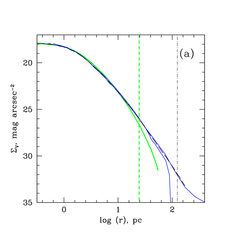
Figure 9.— Final radial profiles of observable quantities (for the time interval $t=2.67\dots 3$ Gyr – the same as in Fig. 8). (a) V-band surface brightness $\Sigma_{V}$. (b) Line-of-sight stellar velocity dispersion $\sigma_{r}$. Thick and thin solid lines (colored green and blue in electronic edition, respectively) correspond to models SDO_n and SDO_b, respectively. (There are two DSO_b profiles: the upper one corresponds to stars along the major axis of the cluster, and the lower one is for stars in the plane perpendicular to the major axis.) Long-dashed lines show the profiles for the model S. Thick vertical short-dashed line marks the value of $r_{m}$ for model SDO_n (see Table 2). Vertical dash-dotted lines correspond to the current tidal radius for SDO models $r_{\rm tid}$. To make these plots we use the projection technique described in Appendix B of Paper I.

In Figure 6a, we show the evolution of the gravitationally bound DM mass for model DO_n (solid thin line). As you can see, tidal stripping is severe in this model, with only $\sim 3.8$% of the total mass surviving as a bound structure after 11 orbits (see Table 2). This behavior is similar to the critical case of Hayashi et al. (2003) with $r_{\rm tid}/r_{s}=2.1$ (see their Fig. 7), which separates their models staying relatively intact (with $r_{\rm tid}/r_{s}>2.1$) and completely disrupted models (with $r_{\rm tid}/r_{s}<2.1$). In our case, this ratio is slightly smaller than 2.1: $r_{\rm tid}/r_{s}=1.73$. Slightly larger resilience to tidal disruption exhibited by our model DO_n can be explained by the fact that Hayashi et al. (2003) used “local Maxwellian approximation” to set up the initial particle distribution in their models, which according to Kazantzidis et al. (2004) leads to artificially high disruption rate for NFW subhalos.

Even for the very last snapshot of model DO_n (at $t=3$ Gyr), the stripped-down subhalo appears to be reasonably stable against total disruption by the tidal forces. Indeed, the binding radius of the remnant $r_{\rm bind}=15$ pc is significantly smaller than the current value of the tidal radius $r_{\rm tid}=56$ pc even at the very end of the simulations. (To estimate $r_{\rm tid}$, we use the actual value of the pericentric distance of $R_{p}=413$ pc which is smaller than the original value of $R_{p}=600$ pc because of the dynamic friction experienced by the subhalo moving in the halo of unbound DM particles.) We expect thus that our NFW subhalo should survive as a gravitationally bound remnant for a few more orbits (and perhaps indefinitely).

The fate of a Burkert DM subhalo orbiting inside a Burkert host galaxy (model DO_b) is completely different, as can be seen in Figure 6b (solid thin line). After only 3 pericentric passages, the subhalo ceases to exist as a coherent structure. To make sure that the failure to find a bound structure after $t=0.79$ Gyr is not an artifact of our halo finding algorithm, we measure both binding radius $r_{\rm bind}=625$ pc and tidal radius $r_{\rm tid}=175$ pc for the last snapshot containing a bound structure. As you can see, at this point the subhalo is bound to be dispersed by tidal forces as its current tidal radius is significantly (almost 4 times) smaller than the binding radius.

Two main conclusions we arrive at in this section are (1) our NFW DM-only subhalo is relatively resilient to total tidal disruption, and (2) a Burkert DM subhalo orbiting inside a Burkert host galaxy is much easier to disrupt that for the case of an NFW DM subhalo orbiting inside an NFW host.

3.5. Tidal Stripping of Hybrid GCs

We are now turning to the results of our two principle models: SDO_n and SDO_b. In these models, a hybrid GC (stars $+$ DM) is orbiting inside the same host galaxies and along the same eccentric orbit as in models DO_n,b. Before being placed in the static potential of the host galaxy, we allow stars and DM to relax in isolation for 120 Myr (model SDO_n) and 170 Myr (model SDO_b).

As you can see in Figure 6, presence of a stellar core, with a mass of mere $\sim 0.9$% of the total mass, inside a DM subhalo makes the subhalo much more resilient to tidal forces disruption. In the case of NFW profile (Figure 6a; see also Table 2), the DM mass of the tidally stripped remnant at $t\simeq 3$ Gyr is 7 times larger in the presence of the stellar core than in the DM-only case. It is also 3 times larger than the mass of the stellar core. For Burkert profile, the difference is even more dramatic: whereas a starless Burkert subhalo is completely disrupted after 3 orbits, the subhalo with a stellar core survives till the end of the simulations, with $\sim 32$% of the total mass of the remnant being in DM form.

Figure 4 provides an explanation for such a marked difference. As we discussed in § 3.3, both NFW and Burkert halos become unbound if instantaneously truncated below a certain radius ($0.77r_{s}$ for NFW profile, and $1.66r_{s}$ for Burkert profile). As you can see in Figure 4, the presence of a stellar GC-like cluster at the center of either halo makes it significantly more bound. In the case of NFW profile (thick solid line), the halo becomes bound for virtually any truncation radius $r$ (being similar in this regard to a singular isothermal sphere). For Burkert halo (thin solid line), there is still a range in truncation radius $r$ where the halo is formally unbound, but the maximum positive value of $E_{\rm tot}$ is significantly lower in the presence of a stellar core. Moreover, for $r\lesssim 0.32r_{s}$ the halo again becomes bound (see Figure 4).

After 7 orbits or $\sim 2$ Gyr, the mass of DM gravitationally bound to the remnant in model SDO_b becomes smaller than the mass of the stellar core. At this point, the rate of the mass loss due to tidal stripping becomes smaller, but still non-negligible (see Figure 6b). We tested the possibility that the observed decrease in bound DM mass after $t\simeq 2$ Gyr is a numerical artifact, caused by a small number ($<10^{4}$) of DM particles attached to the remnant, by resimulating the late evolution of the subhalo in the absence of the static gravitational potential of the host galaxy. For this, we used the gravitationally bound remnant from the $t=2.13$ Gyr snapshot of model SDO_b. The bound DM mass evolution for this additional run is shown with dotted line in Figure 6b. As you can see, in the absence of external tidal field the bound DM mass of the remnant stays virtually constant. It appears thus very unlikely that the late time DM stripping observed in model SDO_b is caused by numerical artifacts (such as evaporation of DM particles due to two-body interactions).

In Figure 7 we show DM column density maps for models SDO_n (left panels) and SDO_b (right panels), for two moments of time: after $\sim 1.5$ orbits (top panels) and after $10-11$ orbits (bottom panels). Two concentric circles show the range of radial distances covered by the models. At the earlier moment of time, you can see a long stream of DM particles, stripped during the first pericentric passage, with a relatively massive bound structure in the center of the stream. At the end of the simulations, multiple streams of stripped particles mix together to create a fuzzy thick disk of DM. The gravitationally bound remnant is barely visible at this point (especially for Burkert model).

In Figure 3 we show averaged DM radial density profiles for $t=1.61\dots 3$ Gyr for models D_n,b (thick solid lines), SD_n,b (thin solid lines), and SDO_n,b (short-dashed lines). As you can see, the DM density in the innermost part of the NFW halo is not modified by external tidal field. Outside of the stars-dominated central region, the DM density profile becomes significantly steeper in the presence of tidal field. At this point, in models SDO_n,b DM is stripped down to the original scale radius $r_{s}$.

Analysis of Table 2 shows that the parameters of our stellar clusters at the end of the simulations are very similar for all our models containing stars (S, SD_n,b, and SDO_n,b). For SD_n and SDO_n models, the presence of relatively large amounts of DM at the center of the cluster leads to somewhat larger values of the central dispersion $\sigma_{c}$ and smaller values of the King core radius $r_{0}$. The value of the apparent mass-to-light ratio $\Upsilon$, defined as (see Paper I)

$$\Upsilon=\frac{9\sigma_{0}^{2}\Upsilon_{\rm GC}}{2\pi G\zeta_{0}R_{hb}},$$ (2)

where $\Upsilon_{\rm GC}\simeq 1.45$ is the assumed baryonic mass-to-light ratio in GCs and $\zeta_{0}$ is the projected stellar surface mass density at the center of the cluster, is larger by $\sim 18$% for a stellar cluster in NFW halo. Overall, the presence of an external tidal field does not seem to change the global structural and dynamic parameters of GCs with DM in a noticeable way.

As can be seen in Figure 2, tidal stripping does not modify significantly the stellar radial density profiles of hybrid GCs: at any moment of time, density profiles for SDO_n,b models (dotted lines) are very close to the density profiles of SD_n,b models (solid lines).

In Figure 8 we show the final radial density profiles for both stars and DM for models SDO_n and SDO_b. As you can see, DM still dominates stars in the outskirts of the stellar cluster. In the stars-dominated area, the DM density profile is steeper because of the adiabatic contraction of DM in the presence of stars. DM density profiles are dramatically modified both by the presence of a stellar core and by tidal stripping.

In model SDO_b, stellar cluster becomes tidally limited by the end of the simulations. By $t=3$ Gyr, around 0.6% of stars (or $\sim 60$ stellar particles) are not gravitationally bound to the cluster, forming distinctive trailing and leading stellar tidal tails. (Conversely, not a single stellar particle has been tidally stripped by $t=3$ Gyr in model SDO_n.) In model SDO_b, the shape of the cluster becomes increasingly non-spherical at large radii at $t\sim 3$ Gyr. As can be seen in Figure 9a, there is an excess of stars in the outskirts of the cluster along its major axis, and a sharp tidal cutoff around the analytical tidal radius $r_{\rm tid}$ near the plane perpendicular to the major axis. (To calculate surface brightness and velocity dispersion profiles for SDO_b model, we used all stellar particles – both bound and unbound.)

As Figure 9a shows, the final surface brightness profiles of the stellar clusters in SDO_n,b models look remarkably similar to the corresponding profiles of Galactic GCs. (We assumed that the baryonic V-band mass-to-light ratio in GCs is $\Upsilon_{\rm GC}=1.45$ – see discussion in Paper I.) The “dent” feature observed in the surface brightness profile of a freshly relaxed hybrid (DM $+$ stars) GC (see Paper I) has been removed in models SDO_n,b by secular evolution of the stellar cluster (see § 3.1). The apparent “tidal” cutoff in the outer surface brightness profile of model SDO_n is caused by the presence of significant amounts of DM in the outskirts of the cluster (similarly to Paper I). In the case of Burkert halo (model SDO_b), the cutoff is of truly tidal nature.

In Figure 9b we show the final line-of-sight velocity dispersion profiles for the stellar clusters in SDO_n,b models. In the case of NFW halo (thick solid line), the line-of-sight velocity dispersion appears to be uniformly inflated by a small factor ($\sim 10$%) across all radii, which can be misinterpreted as a purely stellar cluster with a somewhat larger value of baryonic mass-to-light ratio. For the Burkert halo (thin solid lines), the radial velocity dispersion profile for the stars near the plane perpendicular to the major axis is very close to the profile of a purely stellar cluster, whereas the stars along the major axis show signs of being tidally heated.

4. CONCLUSIONS

DM subhalos with Burkert density profile are much easier to disrupt tidally in the potential of the host galaxy than subhalos with NFW profile. We link this effect to the difference in the binding properties of both types of halos, with the total energy of the Burkert halos becoming positive if truncated at a significantly larger radius than for NFW halos. Setting a low-mass ($\sim 1$% of the total mass) dense stellar core at the center of either NFW or Burkert halo makes them much more resilient to tidal disruption.

Primordial GCs with NFW DM halo can survive severe tidal stripping in the host galaxy, with DM still being the dominant mass component (though not by a large margin) in the tidally stripped-down remnant. DM is concentrated in the outskirts of the remnant. As a result, an apparent “tidal” cutoff in the radial surface brightness profile in isolated warm collapse models (Paper I), caused by the presence of DM, is also present in our tidally stripped NFW model.

We used warm collapse hybrid models to show that neither secular evolution of the stellar cluster nor severe tidal stripping change noticeably the inferred core mass-to-light ratio $\Upsilon$. For both flat-core and cuspy DM halo profiles, $\Upsilon$ stays close to the purely baryonic value.

Tidal stripping can remove almost all DM from primordial GCs with Burkert DM halo. The remaining DM is dynamically unimportant, and cannot prevent stars being stripped off by tidal forces of the host galaxy. This result makes GCs possessing obvious tidal tails (the only known example being Palomar 5) be fully consistent with primordial scenarios of GC formation.

Secular evolution of a DM-dominated GC does not change the main results of Paper I derived for freshly relaxed warm-collapse systems. In particular, in both unevolved and evolved clusters, presence of significant amounts of DM in the outskirts of the cluster manifest itself as a “tidal” cutoff in the outer part of the radial surface brightness profile. It is not clear if the “extratidal” features of cold collapse models from Paper I will be preserved in significantly evolved clusters. As we discussed in § 2.1, simulating a cold-collapse hybrid GC to address this issue is not feasible with the present day technology.

The above results reinforce our conclusion from Paper I that a presence of obvious tidal tails is probably the only observational evidence which can reliably rule out a presence of significant amounts of DM in GCs. (But it cannot rule out primordial scenarios of GC formation.)

To summarize, the results presented in both Paper I and this paper suggest that the whole range of features seen in Milky Way GCs (from apparently truncated profiles of some clusters to the extended tidal tails of Palomar 5) can be consistent with the primordial picture of GC formation, given that there was a range of the initial virial ratios for stellar clusters (from “cold” to “hot” collapses), tidal stripping histories, and/or inner DM density profiles.

References

- Barkana & Loeb (2001) Barkana, R. & Loeb, A. 2001, Physics Reports, 349 (Issue 2), 125
- Beasley et al. (2003) Beasley, M. A., Kawata, D., Pearce, F. R., Forbes, D. A., & Gibson, B. K. 2003, ApJ, 596, L187
- Becker et al. (2001) Becker, R. H., et al. 2001, AJ, 122, 2850
- Bekki & Chiba (2004) Bekki, K. & Chiba, M. 2004, A&A, 417, 437
- Bellazzini, Ferraro, & Ibata (2003) Bellazzini, M., Ferraro, F. R., & Ibata, R. 2003, AJ, 125, 188
- Bromm & Clarke (2002) Bromm, V. & Clarke, C. J. 2002, ApJ, 566, L1
- Burkert (1995) Burkert, A. 1995, ApJ, 447, L25
- Cen (2001) Cen, R. 2001, ApJ, 560, 592
- Dehnen (2000) Dehnen, W. 2000, ApJ, 536, L39
- Grillmair et al. (1995) Grillmair, C. J., Freeman, K. C., Irwin, M., & Quinn, P. J. 1995, AJ, 109, 2553
- Hayashi et al. (2003) Hayashi, E., Navarro, J. F., Taylor, J. E., Stadel, J., & Quinn, T. 2003, ApJ, 584, 541
- Irwin & Hatzidimitriou (1995) Irwin, M. & Hatzidimitriou, D. 1995, MNRAS, 277, 1354
- Kazantzidis et al. (2004) Kazantzidis, S., Magorrian, J., & Moore, B. 2004, ApJ, 601, 37
- Law et al. (2003) Law, D. R., Majewski, S. R., Skrutskie, M. F., Carpenter, J. M., & Ayub, H. F. 2003, AJ, 126, 1871
- Layden & Sarajedini (2000) Layden, A. C. & Sarajedini, A. 2000, AJ, 119, 1760
- Leon, Meylan, & Combes (2000) Leon, S., Meylan, G., & Combes, F. 2000, A&A, 359, 907
- Mashchenko & Sills (2004a) Mashchenko, S. & Sills, A. 2004a, ApJ, 605, L121 (MS04)
- Mashchenko & Sills (2004b) Mashchenko, S. & Sills, A. 2004b, ApJ, in press (preprint astro-ph/0409605) (Paper I)
- McLaughlin (1999) McLaughlin, D. E. 1999, AJ, 117, 2398
- Mizutani, Chiba, & Sakamoto (2003) Mizutani, A., Chiba, M., & Sakamoto, T. 2003, ApJ, 589, L89
- Moore (1996) Moore, B. 1996, ApJ, 461, L13
- Navarro, Frenk, & White (1997) Navarro, J. F., Frenk, C. S., & White, S. D. M. 1997, ApJ, 490, 493
- Odenkirchen et al. (2001) Odenkirchen, M., et al. 2001, AJ, 122, 2538
- Odenkirchen et al. (2003) Odenkirchen, M., et al. 2003, AJ, 126, 2385
- Padoan, Jimenez, & Jones (1997) Padoan, P., Jimenez, R., & Jones, B. 1997, MNRAS, 285, 711
- Peebles (1984) Peebles, P. J. E. 1984, ApJ, 277, 470
- Peebles & Dicke (1968) Peebles, P. J. E. & Dicke, R. H. 1968, ApJ, 154, 891
- Ricotti et al. (2002) Ricotti, M., Gnedin, N. Y., & Shull, J. M. 2002, ApJ, 575, 49
- Rosenblatt, Faber, & Blumenthal (1988) Rosenblatt, E. I., Faber, S. M., & Blumenthal, G. R. 1988, ApJ, 330, 191
- Spergel et al. (2003) Spergel, D. N., et al. 2003, ApJS, 148, 175
- Spitzer (1987) Spitzer, L. 1987, Dynamical Evolution of Globular Clusters (Princeton, NJ: Princeton University Press)
- Springel et al. (2001) Springel, V., Yoshida, N., & White, S. D. M. 2001, New Astronomy, 6, 79
- Tsuchiya, Dinescu, & Korchagin (2003) Tsuchiya, T., Dinescu, D. I., & Korchagin, V. I. 2003, ApJ, 589, L29
- Widrow (2000) Widrow, L. M. 2000, ApJS, 131, 39
- Yoshida et al. (2003) Yoshida, N., Abel, T., Hernquist, L., & Sugiyama, N. 2003, ApJ, 592, 645