Globular Clusters with Dark Matter Halos. I. Initial Relaxation

Abstract

In a series of two papers, we test the primordial scenario of globular cluster formation using results of high-resolutions $N$-body simulations. In this first paper we study the initial relaxation of a stellar core inside a live dark matter minihalo in the early universe. Our dark-matter dominated globular clusters show features which are usually attributed to the action of the tidal field of the host galaxy. Among them are the presence of an apparent cutoff (“tidal radius”) or of a “break” in the outer parts of the radial surface brightness profile, and a flat line-of-sight velocity dispersion profile in the outskirts of the cluster. The apparent mass-to-light ratios of our hybrid (stars $+$ dark matter) globular clusters are very close to those of purely stellar clusters. We suggest that additional observational evidence such as the presence of obvious tidal tails is required to rule out the presence of significant amounts of dark matter in present day globular clusters.

1. INTRODUCTION

The origin of globular clusters (GCs) is one of the important unsolved astrophysical problems. One can divide all proposed scenarios for GC formation into two large categories: 1) in situ formation (when GCs are formed inside their present day host galaxies), and 2) pregalactic formation (when GCs are formed in smaller galaxies which later merge to become a part of the present day host galaxy).

Pregalactic scenarios for GC formation can explain many puzzling properties of GCs in the Milky Way and other galaxies. This is especially true for so-called metal-poor GCs (with $[{\rm Fe/H}]\lesssim-1$), which form a distinctive population in many galaxies. Many of their properties are highly suggestive of their pregalactic origin: low metallicity, large age comparable to the age of the universe, isotropic orbits with the apocentric-to-pericentric distances ratio of $R_{a}/R_{p}\simeq 5.4\pm 3.7$ (Dinescu, Girard, & van Altena, 1999, based on data for 38 metal-poor Galactic GCs) which is consistent with the orbits of dark matter (DM) subhalos ($R_{a}/R_{p}\sim 5\dots 6$) in cosmological $\Lambda$CDM simulations, and a very weak or no correlation with the properties of the host galaxy.

One very interesting variation of the pregalactic picture is the primordial scenario of GC formation, which was first proposed by Peebles & Dicke (1968). In its modern interpretation, the primordial scenario assumes that GCs formed at the center of small DM minihalos in the early universe, before or during the reionization of the universe, which is believed to have ended around the redshift of $z=6$ (Becker et al., 2001). The primordial picture has been considered by many authors, including Peebles (1984), Rosenblatt, Faber, & Blumenthal (1988), Padoan, Jimenez, & Jones (1997), Cen (2001), Bromm & Clarke (2002), and Beasley et al. (2003).

It is usually assumed that during the reionization of the universe no star formation can take place inside small DM halos with the virial temperature below $\sim 10^{4}$ K (or virial mass less than $\sim 10^{8}$ $M_{\odot}$), as the gas in such halos should escape the shallow gravitational potential after being heated to $\sim 10^{4}$ K by the metagalactic Lyman continuum (LyC) background (Barkana & Loeb, 1999). Some authors (Cen, 2001; Ricotti, Gnedin, & Shull, 2002) suggested though, that the reionization of the universe can actually trigger star formation in small DM minihalos through different positive feedback mechanisms. In the scenario of Cen (2001), star formation in small gas-rich minihalos is triggered by radially converging radiation shock fronts caused by the external LyC radiation field. In the cosmological simulations with radiative transfer of Ricotti et al. (2002), small-halo objects constitute the bulk of mass in stars until at least redshift $z\sim 10$ because of the increased non-equilibrium fraction of free electrons in front of the cosmological H ii regions and inside the relic cosmological H ii regions, which results in more efficient H₂ formation and hence cooling of the gas.

Despite the fact that many authors considered different hydrodynamic and radiative processes which can lead to formation of GC-like stellar clusters inside DM minihalos, there has been no detailed study on what happens to such hybrid (GC $+$ DM halo) object after the formation of stars from the point of galactic dynamics. Fully consistent cosmological simulations of structure formation in the universe (such as those of Ricotti et al. 2002), and even higher resolution “semi-consistent” simulations (like in Bromm & Clarke 2002) lack orders of magnitude in spatial and mass resolution to be able to answer the following questions: 1) How does the presence of DM modify the observable properties of GCs? 2) Are there observable features from which the presence of DM in a GC can be inferred? 3) Will DM in “hybrid GCs” survive tidal stripping during the hierarchical assemblage of substructure leading to the formation of large galaxies such as Milky Way?

We try to answer the above questions in a series of two papers. In this first paper, we address the first and the second questions, with the last question being dealt with in the second paper (Mashchenko & Sills, 2004b, hereafter Paper II). Using the $N$-body tree-code GADGET (Springel, Yoshida & White, 2001), we follow the relaxation of initially non-equilibrium stellar clusters inside live DM minihalos around the redshift of $z=7$. Our simulations are collisionless, and can be directly compared with dynamically unevolved GCs; the impact of secular evolution (core collapse) on our results will be explored in Paper II. DM halos have either Navarro, Frenk, & White (1997, hereafter NFW) or Burkert (1995) profiles, and have structural parameters taken from cosmological simulations. We use proto-GC model of Mashchenko & Sills (2004a, hereafter MS04) to set up the initial non-equilibrium configuration of stellar clusters inside DM halos. In MS04 we showed that the collapse of homogeneous isothermal stellar spheres leads to the formation of clusters with the surface brightness profiles being very similar to those of dynamically young Galactic GCs. In this model, all the observed correlations between structural and dynamic parameters of Galactic GCs are accurately reproduced if the initial stellar density $\rho_{i,*}$ and velocity dispersion $\sigma_{i,*}$ had the same universal values: $\rho_{i,*}\simeq 14$ $M_{\odot}$ pc^-3 and $\sigma_{i,*}\simeq 1.91$ km s^-1.

This paper is organized as follows. In Section 2 we describe our method of simulating the evolution of a “hybrid” GC and list the physical and numerical parameters of our models. In Section 3 we show the results of the simulations. Finally, in Section 4 we discuss the results and give our conclusions.

2. MODEL

2.1. Initial Considerations

In our model, GCs with a stellar mass $m_{*}$ are formed at the center of DM halos with the virial mass $m_{\rm DM}$ at the redshift of $z=7$. We fix the mass ratio $\chi\equiv m_{*}/m_{\rm DM}$ to 0.0088. The adopted value of $\chi$ is between the universal baryonic-to-DM density ratio $\Omega_{b}/\Omega_{\rm DM}=0.20$ (Spergel et al., 2003) and the fraction of baryons in GCs in the modern universe of $\simeq 0.0025$ (McLaughlin, 1999). This leaves enough room for such effects as a less than 100% efficiency of star formation in proto-GCs, mass losses due to stellar evolution (through supernovae and stellar winds), a decay of GC systems due to dynamic evolution of the clusters in the presence of tidal fields, and any biased mechanism of GC formation (e.g., when GCs are formed only in DM halos with a low specific angular momentum, like in Cen 2001).

2.2. DM Halos

We consider a flat $\Lambda$CDM universe ($\Omega_{\Lambda}+\Omega_{m}=1$), with the following values of the cosmological parameters: $\Omega_{m}=0.27$ and $H=71$ km s^-1 Mpc^-1 (Spergel et al., 2003). In a flat universe, the critical density can be written as

$$\rho_{c}(z)=\frac{3H^{2}}{8\pi G}\left[\Omega_{m}(1+z)^{3}+1-\Omega_{m}\right].$$ (1)

The virial radius of a DM halo with a virial mass $m_{\rm DM}$ is then as follows:

$$r_{\rm vir}=\frac{1}{1+z}\left(\frac{2\,m_{\rm DM}G\,\Omega_{m}^{z}}{\Delta_{c}H^{2}\,\Omega_{m}}\right)^{1/3},$$ (2)

where the spherical collapse overdensity, $\Delta_{c}$, and the matter density of the universe in units of critical density at the redshift of $z$, $\Omega_{m}^{z}$, are given by

$$\Delta_{c}=18\pi^{2}+82x-39x^{2}$$ (3)

and

$$\Omega_{m}^{z}=\left[1+\frac{1-\Omega_{m}}{\Omega_{m}\,(1+z)^{3}}\right]^{-1}$$ (4)

(Barkana & Loeb, 2001). Here $x\equiv\Omega_{m}^{z}-1$.

We consider two types of DM density profiles: NFW halos and Burkert halos. The NFW model describes reasonably well DM halos from cosmological CDM simulations. It has a cuspy inner density profile with a slope of $\gamma=-1$, and a steeper than isothermal outer density profile:

$$\rho_{n}(r)=\frac{\rho_{0,n}}{r/r_{s}\,(1+r/r_{s})^{2}},$$ (5)

where

$$\rho_{0,n}=\frac{m_{\rm DM}}{4\pi r_{s}^{3}}\left[\ln(1+c)-\frac{c}{1+c}\right]^{-1}.$$ (6)

Here $r_{s}$ and $c\equiv r_{\rm vir}/r_{s}$ are the scale radius and concentration of the halo. Burkert halos, on the other hand, have a flat core. Their outer density profile slope is identical to NFW halos ($\gamma=-3$). This model fits well the rotational curves of disk galaxies (Burkert, 1995; Salucci & Burkert, 2000) and has the following density profile:

$$\rho_{b}(r)=\frac{\rho_{0,b}}{(1+r/r_{s})\,[1+(r/r_{s})^{2}]},$$ (7)

where

$$\rho_{0,b}=\frac{m_{\rm DM}}{2\pi r_{s}^{3}}\left[\ln(1+c)+\frac{1}{2}\ln(1+c^{2})-\arctan c\right]^{-1}.$$ (8)

The concentration $c$ of cosmological halos has a weak dependence on a virial mass (with less massive halos being more concentrated on average). Sternberg, McKee, & Wolfire (2002) give the following expression for a concentration of low mass DM halos in $\Lambda$CDM cosmological simulations at $z=0$, which was obtained from the analysis of halos with the virial masses of $10^{8}\dots 10^{11}$ $M_{\odot}$: $c=27(m_{\rm DM}/10^{9}M_{\odot})^{-0.08}$. Combining this expression with the result of Bullock et al. (2001) that the concentration scales with a redshift as $(1+z)^{-1}$, we obtained the following formula for a concentration of low mass halos at different redshifts:

$$c=\frac{27}{1+z}\left(\frac{m_{\rm DM}}{10^{9}M_{\odot}}\right)^{-0.08}.$$ (9)

Zhao et al. (2003a, b) showed that CDM halos do not have concentrations smaller than $\sim 3.5$, hence equation (9) becomes invalid for halos with $c\lesssim 4$. Sternberg et al. (2002) demonstrated that equation (9) describes very well concentrations of four dwarf disk galaxies from Burkert (1995) fitted by a Burkert profile, so it can be used for both NFW and Burkert halos.

2.3. Stellar Cores

The initial non-equilibrium configuration of proto-GCs was modeled after MS04 as a homogeneous isothermal stellar sphere with isotropic Maxwellian distribution of stellar velocities. Stellar clusters of different mass $m_{*}$ initially had the same universal values of stellar density and velocity dispersion: $\rho_{i,*}=14$ $M_{\odot}$ pc^-3 and $\sigma_{i,*}=1.91$ km s^-1 (MS04). As in MS04, we use a mass parameter $\beta$ to describe different proto-GC models:

$$m_{*}=10^{\beta}\sigma_{i,*}^{3}\left(\frac{375}{4\pi\rho_{i,*}G^{3}}\right)^{1/2},$$ (10)

where $G$ is the gravitational constant. The connection between the initial virial parameter $\nu$ and $\beta$ is $\nu\equiv 2K_{*}/W_{*}=10^{-2\beta/3}$, where $K_{*}$ and $W_{*}$ are initial kinetic and potential energies of the stellar cluster.

Figure 1.— Fraction of stars remaining gravitationally bound after the initial relaxation phase in proto-GC models of MS04. Empty circles mark models with $\beta=-0.6$ (“H”), $\beta=0.4$ (“W”), and $\beta=1.4$ (“C”).

We use models from MS04 to plot in Figure 1 a dependence of the fraction of stars, which form a gravitationally bound cluster after the initial relaxation phase of a proto-GC, on the mass parameter $\beta$ (or the virial parameter $\nu$). Please note that this is the case of no DM (bare stellar cores). As one can see, there are three different regimes of the initial relaxation phase: 1) “Hot” collapse ($-0.7\lesssim\beta\lesssim-0.35$ or $3\gtrsim\nu\gtrsim 1.7$) results in a substantial loss of stars which initial velocity was above the escape speed for the system; only the slowest moving stars collapse to form a bound cluster. 2) “Warm” collapse ($-0.35\lesssim\beta\lesssim 0.85$ or $1.7\gtrsim\nu\gtrsim 0.27$) is very mild and non-violent, and results in virtually no escapers. 3) “Cold” collapse ($\beta\gtrsim 0.85$ or $\nu\lesssim 0.27$) is violent, and leads to increasingly larger fraction of escapers for colder systems. In the last case, the nature of unbinding of stars is very different from the “hot” case. During a cold collapse, the radial gravitational potential is wildly fluctuating. At the intermediate stages of the relaxation, the central potential of the cluster becomes much deeper than the final, relaxed value. As a result, a fraction of stars are accelerated to speeds which will exceed the escape speed of the relaxed cluster. Analysis shows that most of escapers are the stars that initially were predominantly in the outskirts of the cluster and moving in the outward direction.

These three regimes of the initial relaxation of proto-GCs are of very general nature, and are not restricted to the GC formation scenario of MS04. To illustrate that, let us write down an expression for the virial ratio of a homogeneous isothermal sphere, which is applicable to both pre-starburst gas phase of a forming GC, and the initial stellar configuration after the star burst takes place:

$$\nu=\frac{5\langle V^{2}\rangle R}{3GM}.$$ (11)

Here $M$ and $R$ are the mass and the radius of the system, and $\langle V^{2}\rangle$ is the mean-square speed of either gas molecules or stars. Assuming that newly-born stars have the same velocity dispersion as star-forming gas, equation (11) suggests three following physical scenarios resulting in our “hot”, “warm”, and “cold” stellar configurations (in all scenarios we start with an adiabatically contracting gas cloud of a Jeans mass, which corresponds to $\nu_{\rm gas}=1$): 1) non-efficient stars formation with a subsequent loss of the remaining gas leads to our “hot” case, 2) almost 100%-efficient star formation results in the “warm” case, and 3) runaway cooling of the whole cloud on the time scale shorter than the free-fall time, leading to high-efficiency star formation, results in our “cold” case.

Table 1Physical parameters of the models

Model	$\beta$	$\nu_{*}$	$m_{*}$	$r_{*}$	$\tau_{*}$	$r_{*,\rm min}$	$m_{\rm DM}$	$c$	$r_{\rm vir}$	$r_{s}$	$r_{h,\rm DM}$	$\tau_{\rm DM}$	$S$
			$M_{\odot}$	pc	Myr	pc	$M_{\odot}$		pc	pc	pc	Myr
Wn	0.4	0.54	$8.8\times 10^{4}$	11.2	0.49	2.98	$10^{7}$	4.88	885	181	395	52	4.7
Wb	0.4	0.54	$8.8\times 10^{4}$	11.2	0.49	2.98	$10^{7}$	4.88	885	181	436	61	117
Cn	1.4	0.12	$8.8\times 10^{5}$	24.2	0.078	1.57	$10^{8}$	4.06	1906	470	892	56	5.8
Cb	1.4	0.12	$8.8\times 10^{5}$	24.2	0.078	1.57	$10^{8}$	4.06	1906	470	997	66	173
Hn	–0.6	2.5	$8.8\times 10^{3}$	5.21	17	4.14	$10^{6}$	5.87	411	70	174	48	3.7
Hb	–0.6	2.5	$8.8\times 10^{3}$	5.21	17	4.14	$10^{6}$	5.87	411	70	190	55	78

2.4. Physical Parameters of the Models

In this paper, we consider three following initial stellar configurations, which can be considered to be typical “hot”, “warm”, and “cold” cases (see Figure 1): $\beta=-0.6$ (model “H”, stands for “Hot”), $\beta=0.4$ (model “W”, stands for “Warm”), and $\beta=1.4$ (model “C”, stands for “Cold”). We study relaxation of stellar cores in either NFW (suffix “$n$”; e.g., “W_n”) or Burkert (suffix “$b$”) DM halos, which makes up a total of 6 different combinations of stellar cores and DM halos. The physical parameters of these 6 models are summarized in Table 1.

The stellar masses $m_{*}$ in our models cover the whole range of GC masses (see Table 1). The initial stellar radius $r_{*}$ is much smaller than the scale radius of the DM halo $r_{s}$ in all the models. The masses of DM halos $m_{\rm DM}$ range from $10^{6}$ to $10^{8}$ $M_{\odot}$. From Figure 6 of Barkana & Loeb (2001), these DM halos correspond to $1-1.5\sigma$ fluctuations collapsing at the redshift of $z=7$. As one can see, halos in this mass range are populous enough at $z\sim 7$ to account for all observed GCs.

Figure 2.— Redshift dependence of the minimum mass of a stellar core, with the universal initial density $\rho_{i,*}=14$ $M_{\odot}$ pc^-3, which dominates DM at the center of a DM halo. Thick lines (colored green in electronic edition) correspond to stellar cores in NFW halos, whereas thin lines (colored blue in electronic edition) correspond to clusters in Burkert halos. Long-dashed, solid, and short-dashed lines correspond to $\chi=0.0025,0.0088,0.2$.

In all our models, stars initially dominate DM in the core ($S\equiv m_{*}/m_{\rm DM}[r_{*}]>1$, see Table 1), which can be considered as a desirable property for a star formation to take place. It is instructive to check if the above condition ($S>1$) holds for other plausible values of the GC formation redshift $z$ and stellar mass fraction $\chi$. In Figure 2 we show the redshift dependence of the minimum mass of a stellar core in a DM halo, satisfying the condition $S\geq 1$, for a few fixed values of $\chi$ — 0.0025, 0.0088 (our fiducial value), and 0.20. Both NFW (thick lines) and Burkert (thin lines) cases are shown. As one can see, only in the extreme case of an NFW halo at $z=20$ with $\chi=0.0025$ fraction of total mass in stars, the minimum mass of a dominant stellar core $m_{*,\rm min}=1.7\times 10^{3}$ $M_{\odot}$ is approaching the mass range of GCs. The conclusion we arrive at is that, for all plausible values of $z$ and $\chi$, stellar cores with the universal initial density $\rho_{i,*}=14$ $M_{\odot}$ pc^-3 and GC masses dominate DM at the center of DM halos.

2.5. Setting Up $N$-Body Models

DM halos in our models are assumed to have an isotropic velocity dispersion tensor. To generate $N$-body realizations of our DM halos, we sample the following probability density function (PDF) (Widrow, 2000):

$$P(E,R)\propto R^{2}(\Psi-E)^{1/2}F(E).$$ (12)

Here $\Psi$ and $E$ are the relative dimensionless potential and particle energy in units of $4\pi G\rho_{0,n}r_{s}^{2}$ (for NFW halos) and $\pi^{2}G\rho_{0,b}r_{s}^{2}$ (for Burkert halos), $F(E)$ is the phase-space distribution function, and $R\equiv r/r_{s}$ is the dimensionless radial coordinate of the particle. The dimensionless potential $\Psi$ is equal 1 at the center and 0 in infinity. For NFW halos, $\Psi=R^{-1}\ln(1+R)$. For Burkert halos, the corresponding expression is given in Appendix A (eq. [A1]). We use the analytic fitting formulae of Widrow (2000) to calculate $F(E)$ for NFW model, and derive our own fitting formulae for the Burkert profile (see Appendix A). Our models are truncated at the virial radius $r_{\rm vir}$ (eq. [2]): $F(E)=0$ for $r>r_{\rm vir}$. As we will show in § 3.2, this truncation results in an evolution in the outer DM density profile (with the profile becoming steeper for $r\gg r_{s}$), which should not affect our results.

We sample the PDF (eq. [12]) in two steps: 1) A uniform random number $x\in[0\dots 1]$ is generated. The radial distance $R$ is then obtained by solving numerically one of the two following non-linear equations:

$$\ln(1+R)-R/(1+R)=x\,[\ln(1+c)-c/(1+c)]$$ (13)

for the NFW profile and

$$\ln(1+R)+[\ln(1+R^{2})]/2-\arctan R=$$

$$=x\left[\ln(1+c)+[\ln(1+c^{2})]/2-\arctan c\right]$$ (14)

for the Burkert profile. 2). Given $R$, we can calculate $\Psi$. Instead of equation (12), we can now sample the following PDF:

$$P(E)\propto\Pi\equiv\left(\frac{\Psi-E}{\Psi}\right)^{1/2}\frac{F(E)}{F(\Psi)}.$$ (15)

As $F(E)$ is a monotonically increasing function and $0\leq E\leq\Psi$, the following inequality holds: $0\leq\Pi\leq 1$. Two uniform random numbers, $y\in[0\dots 1]$ and $E\in[0\dots\Psi]$, are generated. If $y\leq\Pi$, we accept the value of the dimensionless energy $E$; otherwise, we go back to the previous step (generation of $y$ and $E$).

The velocity module $\upsilon$ can be obtained from the equation for the total energy of a particle: $E=\upsilon^{2}/2+\Psi$. Finally, two spherical coordinates angles $\theta$ and $\varphi$ are generated for both radius and velocity vectors using the following expressions: $\cos\theta=2t-1$ and $\varphi=2\pi u$. (Here $t$ and $u$ are random numbers distributed uniformly between 0 and 1.)

The above method to generate $N$-body realizations of either NFW or Burkert halos does not use a “local Maxwellian approximation” to assign velocities to particles. Instead, it explicitly uses phase-space distribution functions, which was shown to be a superior way of setting up $N$-body models (Kazantzidis, Magorrian, & Moore, 2004).

Stellar cores are set up as homogeneous spheres at the center of DM halos: $R=r_{*}x^{1/3}$, where $x\in[0\dots 1]$ is a uniformly distributed random number. We use equal mass stellar particles. Velocities of the particles have a Maxwellian distribution. The components of the radius and velocity vectors are generated in the same fashion as for DM particles.

2.6. Numerical Parameters of the Models

Table 2Numerical parameters of the models

Model	$N_{*}$	$\epsilon_{*}$	$N_{\rm DM}$	$\epsilon_{\rm DM}$	$t_{1}$	$t_{2}$	$\Delta t_{\rm max}$	Note
		pc		pc	Myr	Myr	Myr
W0	$10^{5}$	0.15	$\cdots$	$\cdots$	190	370	0.3	1
WnS	$10^{4}$	0.30	$\cdots$	$\cdots$	95	190	0.2	2
Wn	$10^{4}$	0.30	$10^{6}$	1.5	200	250	0.2	$\cdots$
WbS	$10^{4}$	0.30	$\cdots$	$\cdots$	95	190	0.2	2
Wb	$10^{4}$	0.30	$10^{6}$	1.5	150	250	0.2	$\cdots$
C0	$10^{5}$	0.32	$\cdots$	$\cdots$	56	92	0.3	1
Cn	$10^{5}$	0.32	$5\times 10^{5}$	4.7	130	190	0.2	$\cdots$
Cb	$10^{5}$	0.32	$5\times 10^{5}$	5.2	95	190	0.2	$\cdots$
H0	$10^{5}$	0.069	$\cdots$	$\cdots$	1300	1800	0.3	1
Hn	$10^{4}$	0.15	$5\times 10^{5}$	1.7	1500	3700	20	$\cdots$
Hb	$10^{4}$	0.15	$5\times 10^{5}$	1.8	1500	3700	20	$\cdots$

In addition to 6 models from Table 1 which consist of a live DM halo plus a stellar core, we also ran 2 more models with a static DM potential (marked with the letter “S” at the end). The numerical parameters for these 8 models are listed in Table 2. In this table we also list parameters for the three properly rescaled stars-only models from MS04 (H₀, W₀, and C₀), which will be used as reference cases.

To run our models, we use a parallel version of the multistepping tree code GADGET-1.1 (Springel et al., 2001). The code allows us to handle separately stellar and DM particles, with each species having a different softening length — $\epsilon_{*}$ and $\epsilon_{\rm DM}$, respectively. We slightly modified the code by introducing an optional static DM potential (either NFW, or Burkert).

The values of the softening lengths were chosen to be comparable with the initial average interparticle distance. We used the following expression for the stellar particles: $\epsilon=0.77r_{h}N^{-1/3}$ (Hayashi et al., 2003), where the half-mass radius $r_{h}$ was measured at the initial moment of time (so $r_{h}=r_{*}/2^{1/3}$). The same expression was used to calculate $\epsilon_{\rm DM}$ for H_n,b models, whereas for the models W_n,b and C_n,b we used half of the value given by the equation of Hayashi et al. (2003) to achieve a better spatial resolution within the stellar core.

Aarseth, Lin, & Papaloizou (1988) showed that collapsing homogeneous stellar spheres with a non-negligible velocity dispersion $\sigma_{i,*}$ do not experience a fragmentation instability (and as a consequence preserve orbital angular momentum of stars), if the following condition is met: $N_{*}\gtrsim[m_{*}/(r_{*}\sigma_{i,*}^{2})]^{3}$, where $N_{*}$ is the number of stars. For our models, this adiabaticity criterion can be rewritten as

$$\log N_{*}\gtrsim 2\beta+3\log 5.$$ (16)

As we discussed in MS04, if real GCs indeed started off as isothermal homogeneous stellar spheres, they should have collapsed adiabatically. We also showed that if both the condition in equation (16) and $\epsilon_{*}\lesssim 0.25r_{*,\rm min}$ are met, the results of simulations of collapsing stellar spheres do not depend on the number of particles $N_{*}$ and the softening length $\epsilon_{*}$. (Here $r_{*,\rm min}$ is the minimum half-mass radius of the cluster during the collapse.) By comparing Tables 1 and 2 one can see that the values of $N_{*}$ and $\epsilon_{*}$ we use in our simulations meet both above conditions.

The evolution time $t_{2}$ in our runs is at least 3 times longer than the crossing time for DM $\tau_{\rm DM}$, and hundreds and even thousands times longer than the crossing time for stellar particles $\tau_{*}$ (see Tables 1 and 2). As we will see in the next section, this time is enough for stellar and DM density profiles to converge. On the other hand, it is short enough to avoid significant dynamic evolution in the stellar clusters caused by encounters between individual particles.

The individual time steps in the simulations are equal to $(2\eta\epsilon/a)^{1/2}$, where $a$ is the acceleration of a particle, and parameter $\eta$ controls the accuracy of integration. We used a very conservative value of $\eta=0.0025$ and set the maximum possible individual time step $\Delta t_{\rm max}$ value to either 20 or 0.2 Myr (see Table 2). As a result, the accuracy of integration was very high: $\Delta E_{\rm tot}\lesssim 0.06$%, where $\Delta E_{\rm tot}$ is the maximum deviation of the total energy of the system from its initial value. One has to keep in mind though that numerical artifacts are the most pronounced in the central densest area, where the frequency of strong gravitational interaction between particles is the highest. We estimate the severity of these effects by looking at the total energy conservation in our purely stellar models from MS04: in models H₀, W₀, and C₀ the values of $\Delta E_{\rm tot}$ are $\sim 0.05$%, $\sim 0.85\%$, and $\sim 0.8$% (for the model W₀ we used a larger value of $\eta=0.02$, hence the relatively large errors). As you can see, even though the numerical artifacts in the dense stellar cluster are more visible than in the DM $+$ a stellar core case, the magnitude of these effects is still reasonably low.

For completeness sake, we also give the values of other code parameters which control the accuracy of simulations: ErrTolTheta=0.6, TypeOfOpeningCriterion=1, ErrTolForceAcc=0.01, MaxNodeMove=0.05, TreeUpdateFrequency=0.1, and DomainUpdateFrequency=0.2. (Please see the code manual for explanation of these parameters). The code was compiled with the option DBMAX enabled, which allowed it to use a very conservative node-opening criterion.

3. RESULTS OF SIMULATIONS

3.1. General Remarks

Table 3Parameters for relaxed stellar clusters

Model	$r_{h,*}$	$\sigma_{c}$	$\rho_{c}$	$R_{h,*}$	$R_{hb}$	$\sigma_{0}$	$\Sigma_{V}$	$r_{0}$	$f_{0}$	$\Upsilon$	$r_{\rho}$	$r_{m}$
	pc	km s-1	$M_{\odot}$ pc3	pc	pc	km s-1	mag arcsec-2	pc		$M_{\odot}$ $L_{\odot}^{-1}$	pc	pc
W0	4.64	4.07	310	3.64	2.77	3.84	18.71	3.01	0.226	1.43	$\cdots$	$\cdots$
WnS	4.51	4.36	360	3.50	2.63	4.11	18.63	2.96	0.253	1.60	$\cdots$	$\cdots$
Wn	4.08	4.83	500	3.16	2.31	4.55	18.39	2.78	0.279	1.80	7.74	19.7
WbS	4.67	4.05	310	3.64	2.81	3.83	18.73	2.98	0.238	1.43	$\cdots$	$\cdots$
Wb	4.65	4.12	350	3.61	2.54	3.89	18.65	2.86	0.229	1.52	17.8	54.7
C0	2.55	14.4	$1.3\times 10^{4}$	2.03	1.52	13.6	15.31	1.64	0.241	1.43	$\cdots$	$\cdots$
Cn	4.50	14.3	$1.1\times 10^{4}$	3.54	1.55	13.4	15.45	1.75	0.166	1.55	10.0	44.0
Cb	4.50	14.4	$1.3\times 10^{4}$	3.52	1.49	13.5	15.30	1.62	0.168	1.42	27.6	125
H0	20.2	0.54	0.71	14.9	7.13	0.51	24.28	8.29	0.154	1.64	$\cdots$	$\cdots$
Hn	5.47	1.57	25	4.20	2.79	1.56	21.44	4.06	0.329	2.88	$\cdots$	$\cdots$
Hb	11.5	0.97	4.8	8.84	4.43	0.97	22.70	5.71	0.212	2.23	10.4	18.2

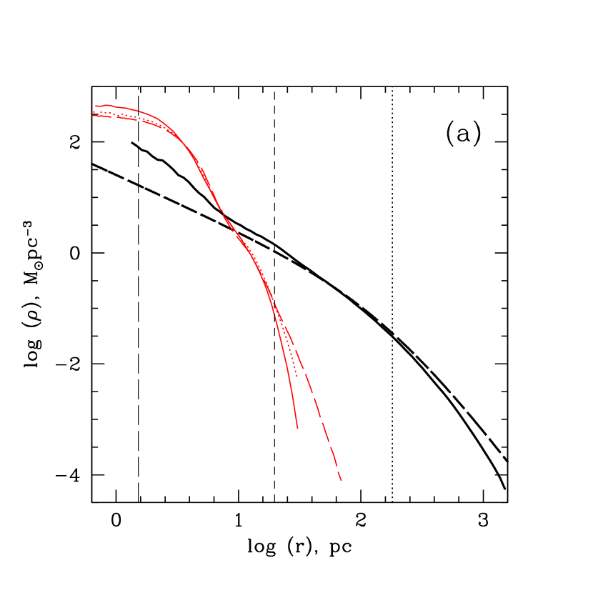
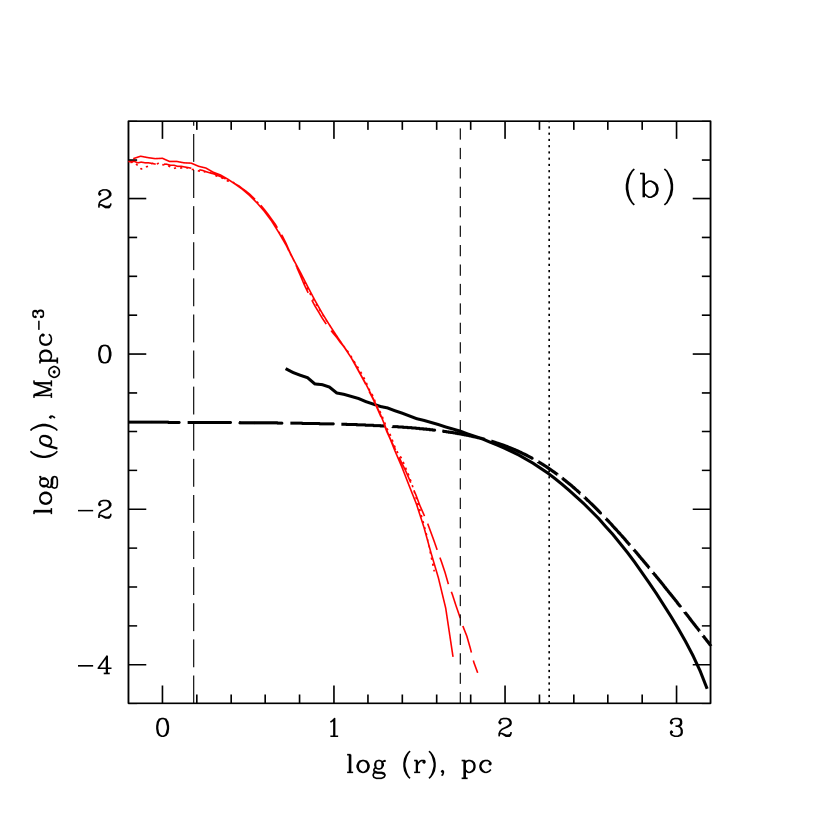
Figure 3.— Radial density profiles for warm collapse models. (a) The case of NFW halo. (b) The case of Burkert halo. Thick lines correspond to DM density; thin lines (colored red in electronic edition) show stellar density. Solid lines correspond to the cases of a live DM halo $+$ a stellar core (models W_n and W_b), long-dashed lines depict analytic DM profiles and a relaxed stellar cluster profile in the absence of DM (model W₀), and dotted lines show stellar density profiles for static DM models (W_nS and W_bS). Vertical long-dashed, short-dashed, and dotted lines mark the values of $\epsilon_{\rm DM}$, $r_{m}$, and $r_{s}$.

For each of our models, we generated 100–200 individual timeframe snapshots. The last 20–60% of the snapshots (corresponding to the time interval $t_{1}\dots t_{2}$, see Table 2) were used to calculate the properties of relaxed models, including radial profiles and different stellar cluster parameters listed in Table 3. In all snapshots, we removed in an iterative manner the escapers (particles whose velocity exceeds the escape velocity $V_{\rm esc}=[-2\Phi]^{1/2}$, where $\Phi$ is the local value of the gravitational potential). This procedure affected models from MS04 (H₀, W₀, and C₀), and DM particles only in the models presented here. One of the reasons for removing escapers was to make the results of the simulations directly comparable with the results from Paper II where this procedure is applied to discount particles stripped by tidal forces.

The radial profiles shown in this section were obtained by averaging the corresponding profiles from individual snapshots in the time interval $t_{1}\dots t_{2}$. For each profile, we only show the part which is sufficiently converged (the dispersion between different snapshots is very small). For projected quantities (such as surface brightness $\Sigma_{V}$ and line-of-sight velocity dispersion $\sigma_{r}$) we use the projection method described in Appendix B which produces much less noisy radial profiles than a straightforward projection onto one plane or three orthogonal planes. This is crucial for the analysis of the properties of the outer, low density parts of stellar clusters, which is the main purpose of this study.

The virial ratio $\nu$ for our models is consistent with unity within the measurement errors at the end of simulations. All the global model parameters (listed in Table 3) converge to their final values by $t=t_{2}$. Similarly, radial density and velocity dispersion profiles converge to their final form over a wide range of radial distances. We explicitly checked that the evolution time $t_{2}$ is more than three crossing times at the largest radius for stellar density profiles shown in Figures 3, 5, and 7. All the above let us conclude that the results presented here are collisionless steady-state solutions.

3.2. Warm Collapse

In the absence of DM, an isothermal homogeneous stellar sphere with the mass parameter $\beta=0.4$ relaxes to its equilibrium state with virtually no stars lost (see Figure 1). This makes it an interesting case to test the result of Peebles (1984), that a stellar cluster inside a static constant density DM halo can acquire a radial density cutoff similar to that expected from the action of tidal forces of the host galaxy, for the case of live DM halos with cosmologically relevant density profiles and initially non-equilibrium stellar cores.

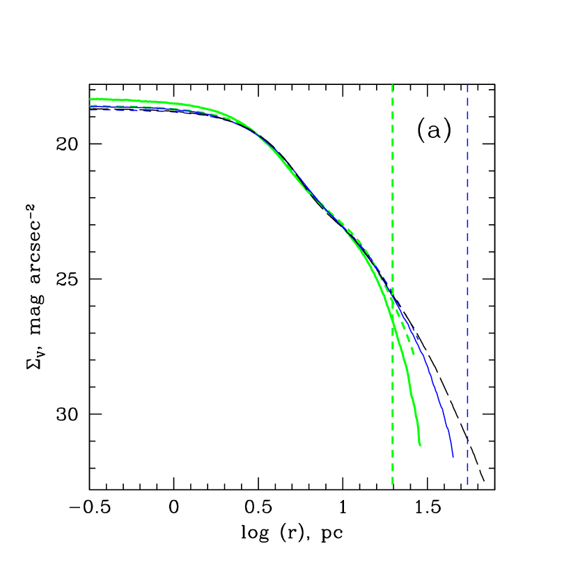
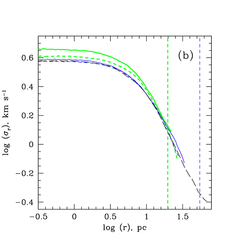
Figure 4.— Radial profiles of observable quantities for warm collapse models. (a) Surface brightness $\Sigma_{V}$. (b) Line-of-sight velocity dispersion $\sigma_{r}$. Thick lines (colored green in electronic edition) correspond to NFW cases; thin lines (colored blue in electronic edition) correspond to Burkert cases. Solid lines show profiles for models W_n and W_b, short-dashed lines correspond to models W_nS and W_bS, and long-dashed lines correspond to model W₀. Vertical short-dashed lines mark the values of $r_{m}$.

In Figure 3 we show the radial density profiles for relaxed stellar core and DM halo, both for NFW model (panel a) and Burkert model (panel b), for the case of a warm collapse (“W” models). Here long-dashed lines show the density profiles for stars in the absence of DM (thin lines) and DM in the absence of stars (thick lines). Solid lines, on the other hand, show the density profiles for stars and DM having been evolved together. We also show as dotted lines the stellar radial density profiles for the case of a static DM potential.

As you can see from Figure 3, in the absence of DM (model W₀), the relaxed stellar cluster has a central flat core and a close to power-law outer density profile. The radial density profile has also a small “dent” outside of the core. It is not a transient feature (in the collisionless approximation), as the virial ratio for the whole cluster is equal to unity within the measurements errors ($\nu=1.001\pm 0.005$ for $t=t_{1}\dots t_{2}$) and the evolution time is $>7$ crossing times even at the very last radial density profile point. As we show in Paper II, collisional long-term dynamic evolution of a cluster will remove this feature, bringing the overall appearance of the density profile closer to that of the majority of observed GCs. The central stellar density in the model W₀ is $\sim$ three orders of magnitude larger than the central density of DM in the undisturbed Burkert halo, and becomes comparable to the density of the undisturbed NFW halo only at very small radii $r\lesssim 0.1$ pc (which is outside of the range of radial distances in Figure 3a).

In the case of a live DM halo coevolving with the stellar core, the DM density profile is significantly modified within the central area dominated by stars (see Figure 3). In both NFW and Burkert halos, DM is adiabatically compressed by the potential of the collapsing stellar cluster to form a steeper slope in the DM radial density profile. The slope of the innermost part of the DM density profile is $\gamma\simeq-1.5$ for the NFW halo and $\gamma\simeq-1.0$ for the Burkert halo. The lack of resolution does not allow us to check if the slope stays the same closer to the center of the DM halos.

In the outer parts of the DM halos (beyond the scale radius $r_{s}$, which is marked by vertical dotted lines in Figure 3), the DM density profile becomes steeper than the original slope of $\gamma=-3$. This can be explained by the fact that our DM halo models are truncated at a finite radius $r_{\rm vir}$ and hence are not in equilibrium. It should bear no effect on our results, as in all our models stellar clusters do not extend beyond $r_{s}$.

As you can see in Figure 3, the impact of the presence of a live DM halo on the stellar density profile is remarkably small (especially for the Burkert halo). In the presence of DM, the central stellar density becomes somewhat larger (by $\sim 60$% and $\sim 10$% for the NFW and Burkert halos, respectively; see Table 3).

The most interesting effect is observed in the outer parts of the stellar density profiles, where the slope of the profiles becomes significantly larger than that of a purely stellar cluster, which is similar to the result of Peebles (1984). The density profile starts deviating from the profile for the model W₀ somewhere between the radius $r_{\rho}$ and the radius $r_{m}$ (where the enclosed masses for stars and DM become equal, see Table 3).

There is a simple explanation for the steepening of the stellar density profile seen in Figure 3 around the radius $r_{m}$. In the absence of DM, warm collapse of a homogeneous stellar sphere (our model W₀) is violent enough to eject a number of stars into almost radial orbits, forming a halo of the relaxed cluster. In the case when the DM halo is present, dynamics does not change much near the center of the cluster where stars are the dominant mass component. Around the radius $r_{m}$ the enclosed DM mass becomes comparable to that of stars. As a result, gravitational deceleration, experienced by stars ejected beyond $r_{m}$, more than doubles, resulting in a significantly smaller number of stars populating the outer stellar halo at $r>r_{m}$. This should lead to significantly steeper radial density profile beyond $r_{m}$, as observed in our W_n,b models.

As in Peebles (1984) model, in our model the steepening of the stellar density profile is caused by the fact that at large radii the gravitational potential is dominated by DM. The principal difference between the two models is that in Peebles (1984) the stellar cluster is assumed to be isothermal and in equilibrium; our clusters are not in equilibrium initially, and their final equilibrium configuration is not isothermal (stars are dynamically colder in the outskirts of the cluster).

To allow a direct comparison of the model results with observed GCs, in Figure 4 we plot both the surface brightness $\Sigma_{v}$ profile (panel a) and the line-of-sight velocity dispersion $\sigma_{r}$ profile (panel b) for warm collapse models. The surface brightness $\Sigma_{V}$ in units of mag arcsec^-2 is calculated using the following formula:

$$\Sigma_{v}=V_{\odot}-2.5[\log(\zeta/\Upsilon_{\rm GC})+2-2\log(3600\times 180/\pi)].$$ (17)

Here $V_{\odot}=4\fm 87$ is the absolute $V$-band magnitude of the Sun, $\zeta$ is the projected surface mass density in units of $M_{\odot}$ pc^-2, and $\Upsilon_{\rm GC}$ is the assumed $V$-band mass-to-light ratio for baryons in GCs. For $\Upsilon_{\rm GC}$ we adopt the observationally derived averaged value of 1.45 from McLaughlin (1999), which is also between the two stellar-synthesis model values (1.36 for the Salpeter and 1.56 for the composite — with a zero slope for stellar masses $<0.3$ $M_{\odot}$ — initial mass functions) of Mateo et al. (1998).

As you can see in Figure 4, the presence of a DM halo introduces an outer cutoff in the surface brightness radial profile of stellar cluster, which makes the profile look very similar to a King model profile. Interestingly, stellar cluster evolving in a live NFW DM halo acquires even steeper outer density and brightness profiles than for the case of a static DM potential (see Figures 3a and 4a).

Analysis of the line-of-sight velocity dispersion profiles for warm collapse models (Figure 4b) shows that the presence of a DM halo slightly inflates the value of $\sigma_{r}$ in the core of the cluster (by $\lesssim 20$%, see Table 3). The outer dispersion profile either stays unchanged (as in the case of the Burkert halo), or becomes slightly steeper (for the NFW model). The static DM models present profiles of an intermediate type.

A slight increase of $\sigma_{r}$ in the central part of the cluster can be misinterpreted observationally as a GC with no DM which has a bit larger value of the baryonic mass-to-light ratio $\Upsilon$. To quantify this effect, we apply a core fitting (or King’s) method of finding the central value of $\Upsilon$ in spherical stellar systems (Richstone & Tremaine, 1986):

$$\Upsilon=\frac{9\sigma_{0}^{2}}{2\pi GI_{0}R_{hb}}.$$ (18)

Here $I_{0}$ is the central surface brightness in physical units. We assume here that $I_{0}=\zeta_{0}/\Upsilon_{\rm GC}$, where $\zeta_{0}$ is the projected surface mass density at the center of the model cluster. The core fitting method assumes that the mass-to-light ratio is independent of radius, which is obviously not true for our stars $+$ DM models. In our models the stellar particles have the same mass, so there is no radial mass segregation between high and low mass stars caused by the long-term dynamic evolution of the cluster. As a result, the equation (18) should not be used to compare our models with real GCs. Instead, we use it to check if there is a change in the apparent mass-to-light ratio $\Upsilon$ between our purely stellar models and the models containing DM. We list the values of $\Upsilon$ for different models in Table 3. As you can see, in the case of NFW halo (model W_n), the presence of the DM halo leads to $\sim 25$% increase in the value of the apparent mass-to-light ratio. Such a small increase is well within the observed dispersion of $\Upsilon$ values for Galactic GCs (Pryor & Meylan, 1993). In the case of the Burkert halo, the apparent central mass-to-light ratio is only $\sim 6$% larger than for the purely stellar model.

3.3. Cold Collapse

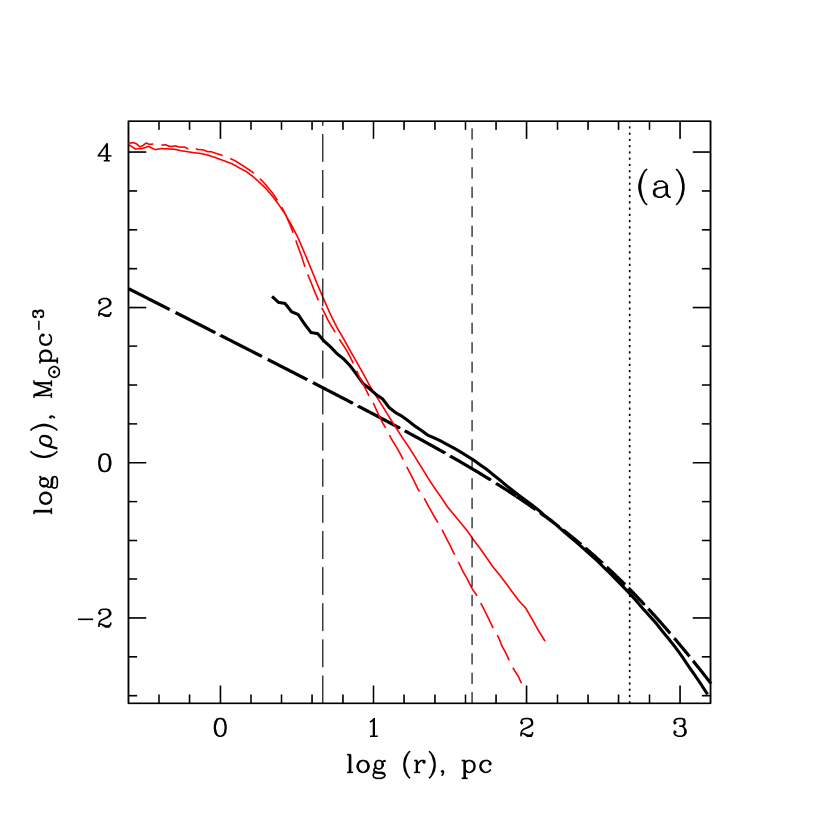
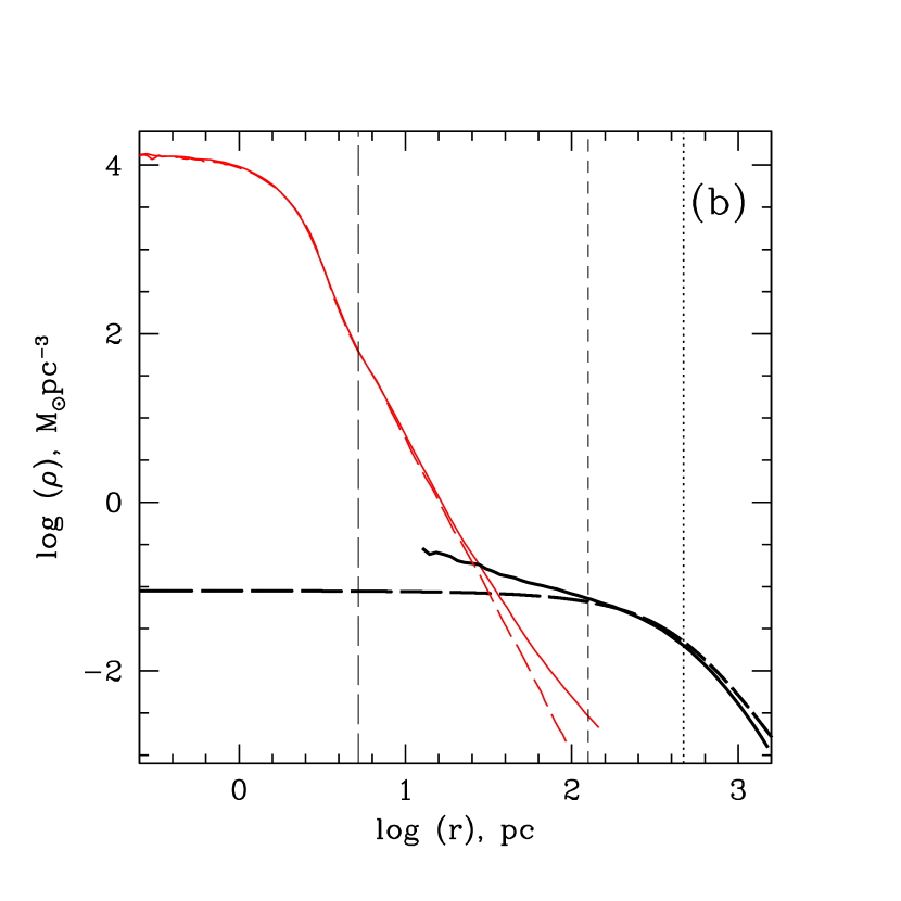
Figure 5.— Radial density profiles for cold collapse models. (a) The case of NFW halo. (b) The case of Burkert halo. Thick lines correspond to DM density; thin lines (colored red in electronic edition) show stellar density. Solid lines correspond to the cases of a live DM halo $+$ a stellar core (models C_n and C_b); long-dashed lines depict analytic DM profiles and a relaxed stellar cluster profile in the absence of DM (model C₀). Vertical long-dashed, short-dashed, and dotted lines mark the values of $\epsilon_{\rm DM}$, $r_{m}$, and $r_{s}$.

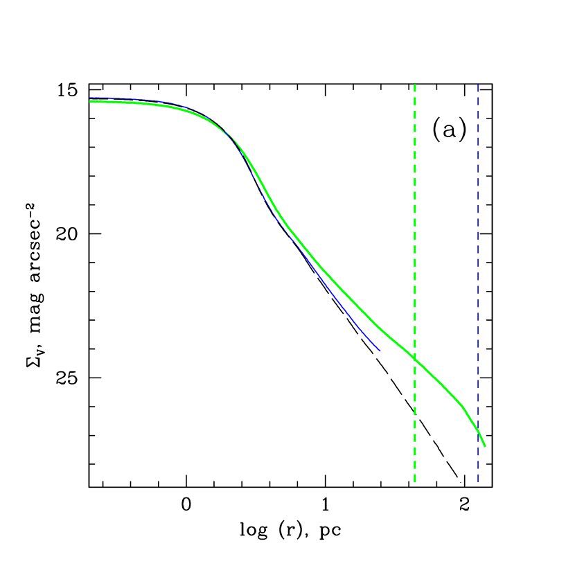
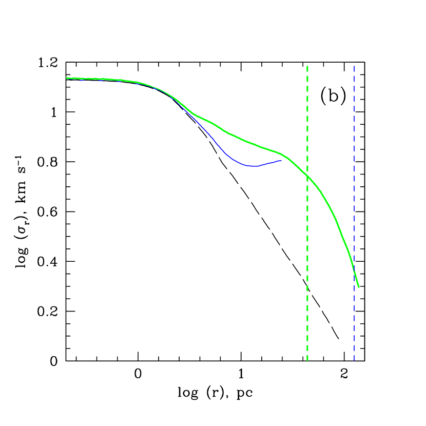
Figure 6.— Radial profiles of observable quantities for cold collapse models. (a) Surface brightness $\Sigma_{V}$. (b) Line-of-sight velocity dispersion $\sigma_{r}$. Thick lines (colored green in electronic edition) correspond to NFW cases; thin lines (colored blue in electronic edition) correspond to Burkert cases. Solid lines show profiles for models C_n and C_b; long-dashed lines correspond to model C₀. Vertical short-dashed lines mark the values of $r_{m}$.

A principal difference between warm and cold collapse models from MS04 is that in the cold collapse case a significant fraction of stars becomes unbound after the initial relaxation phase (see Figure 1). In our model C₀ with the mass parameter $\beta=1.4$ the fraction of the stars lost is 30%. The radial density profile for C₀ model is similar to that of W₀ model (see Figure 5). One can intuitively expect the escapers from the model C₀ to be trapped inside our models containing DM, forming a distinctive feature in the outer density and velocity dispersion profiles.

As you can see in Figures 5 and 6, our cold collapse models do show such features. Both density and surface brightness profiles become more shallow in the outer parts of the stellar clusters where DM dominates stars. This is valid for both NFW and Burkert halos. For the NFW and Burkert cases, the slope of the outer stellar density profile is $\gamma=-2.6$ and $-2.2$, respectively. For the purely stellar case (model C₀) the slope is $\gamma=-3.8$, so the relative change in the slope is $\Delta\gamma=1.2$ and $1.6$ for the NFW and Burkert cases. This behavior is mimicked by the corresponding surface brightness profiles (Figure 6a). It is interesting to note that, for the C_n model the radial $\Sigma_{V}$ profile exhibits a significant steepening of the slope in the outmost parts of the cluster, creating an appearance of a “tidal cutoff” (similarly to the warm collapse cases).

Even more pronounced are features in the line-of-sight velocity dispersion profiles (Figure 6b). In both NFW and Burkert cases, there is a plateau in the radial $\sigma_{r}$ profiles around the radius $r_{m}$ where DM becomes the dominant mass component. The apparent “break” in the surface brightness profile and accompanying flattening of the radial $\sigma_{r}$ profile, seen in our models containing DM, can be misinterpreted observationally as a presence of “extratidal” stars heated by the tidal field of the host galaxy.

Similarly to warm collapse models, the apparent mass-to-light ratio $\Upsilon$ for cold collapse models in the presence of a live DM halo is very close to the purely stellar case C₀ (see Table 3). Interestingly, the half-mass radii for warm and cold collapse models with DM are almost identical. This is consistent with the properties of the observed GCs, which have comparable half-mass radii for a wide range of cluster masses.

DM density profiles for the cold collapse cases (Figure 5) exhibit a very similar behavior to the warm collapse models in the stars dominated central region. For both NFW and Burkert halos, the innermost slopes of the density profiles become steeper ($\gamma\simeq-1.8$ and $-0.6$, respectively) in the presence of a stellar core. The NFW DM density profile shows a break around the radius $r_{m}$.

As you can see in Table 3 and Figure 5, the final stellar cluster half-mass radius is smaller than the DM softening length $\epsilon_{\rm DM}\sim 5$ pc. We reran models C_n and C_b with much smaller value of $\epsilon_{\rm DM}=1$ pc to test the possibility that our results were influenced by the fact that DM is not resolved on the stellar cluster scale. For both C_n and C_b, the relaxed stellar profiles are found to be virtually identical to the cases with larger $\epsilon_{\rm DM}$. In particular, a “kink” seen in Figures 5a and 5b around the radius $\epsilon_{\rm DM}$ is also present at the same location in the simulations with much smaller value of $\epsilon_{\rm DM}$, and is definitely not a numerical artifact. In the case of NFW halo, the central stellar velocity dispersion becomes slightly larger, which results in somewhat larger value of $\Upsilon=1.88$. This could be in part because of artificial mass segregation, which should be more pronounced in the case of $\epsilon_{\rm DM}$ being significantly lower than the optimal value (in our cold collapse models, DM particles are $\sim 20$ times more massive than stellar particles). As a result, the actual $\Upsilon$ value could be even closer to the baryonic value. In the case of Burkert halo with $\epsilon_{\rm DM}=1$ pc, the core mass-to-light ratio $\Upsilon=1.45$, which is identical to the case of no DM. We conclude that our choice of $\epsilon_{\rm DM}$ did not affect the main results presented in this Section.

3.4. Hot Collapse

It is generally assumed that in an equilibrium star-forming cloud no bound stellar cluster will be formed after stellar winds and supernova explosions expel the remaining gas if the star formation efficiency is less than 50% (which corresponds to the initial virial parameter for the stellar cluster of $\nu>2$). In MS04 we showed that it is not true for initially homogeneous stellar clusters which have a Maxwellian distribution of stellar velocities. In such clusters with the initial virial parameter as large as 2.9 (corresponding to the mass parameter $\beta$ as low as $-0.7$), a bound cluster, containing less than 100% of the total mass, is formed by the slowest moving stars. (A similar conclusion was reached by Boily & Kroupa 2003 for initially polytropic stellar spheres.)

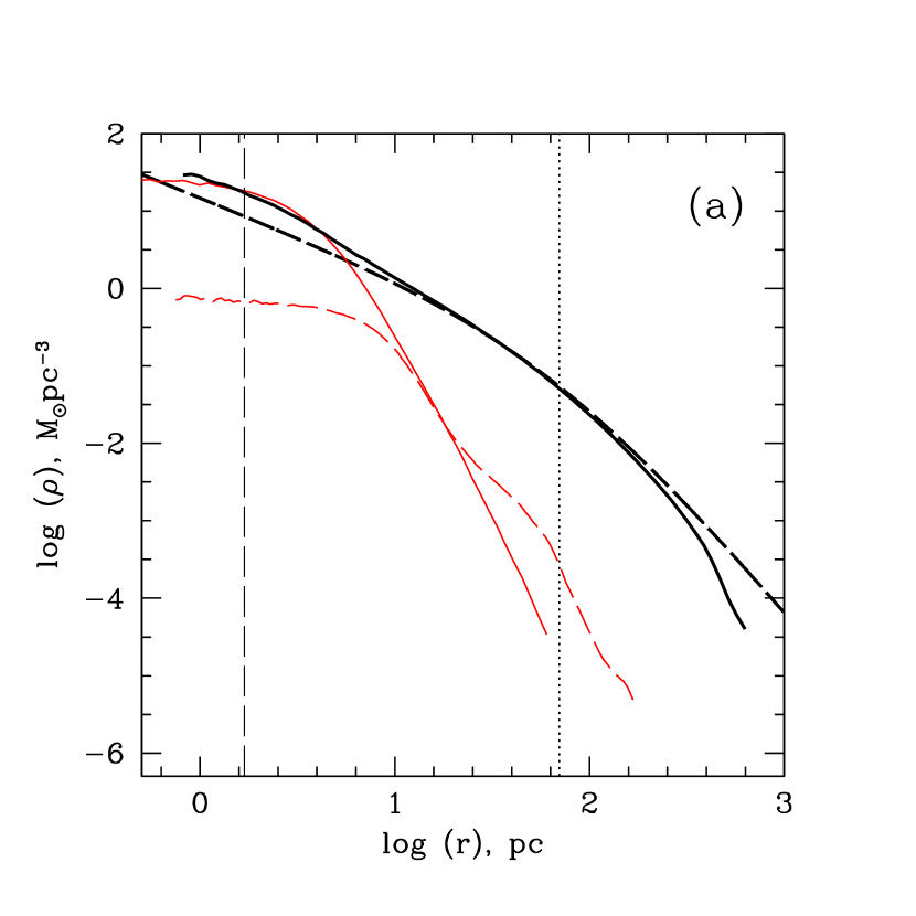
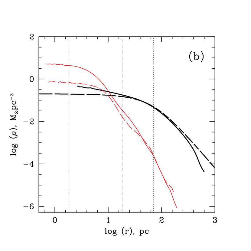
Figure 7.— Radial density profiles for hot collapse models. (a) The case of NFW halo. (b) The case of Burkert halo. Thick lines correspond to DM density; thin lines (colored red in electronic edition) show stellar density. Solid lines correspond to the cases of a live DM halo $+$ a stellar core (models H_n and H_b); long-dashed lines depict analytic DM profiles and a relaxed stellar cluster profile in the absence of DM (model H₀). Vertical long-dashed, short-dashed, and dotted lines mark the values of $\epsilon_{\rm DM}$, $r_{m}$ (only the Burkert case is shown, as in the NFW case the enclosed DM mass is larger than that of stars at any radius), and $r_{s}$.

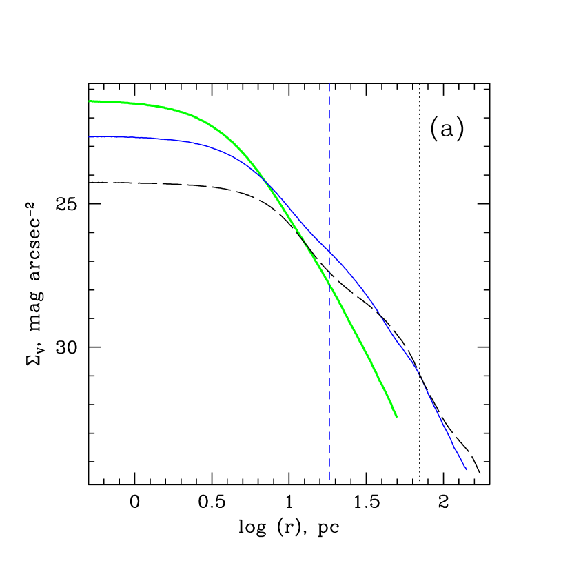
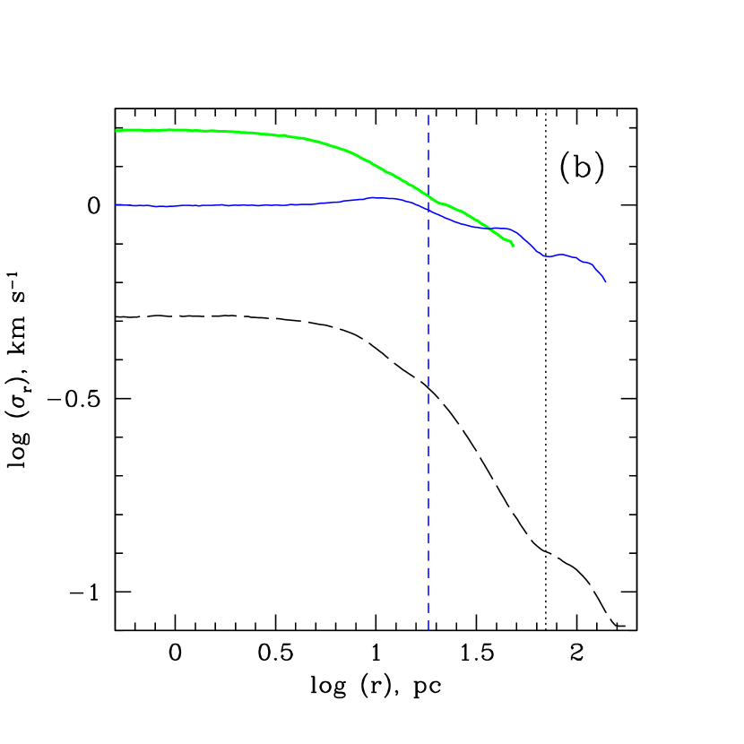
Figure 8.— Radial profiles of observable quantities for hot collapse models. (a) Surface brightness $\Sigma_{V}$. (b) Line-of-sight velocity dispersion $\sigma_{r}$. Thick lines (colored green in electronic edition) correspond to NFW cases; thin lines (colored blue in electronic edition) correspond to Burkert cases. Solid lines show profiles for models H_n and H_b; long-dashed lines correspond to model H₀. Vertical short-dashed line marks the value of $r_{m}$ (only the Burkert case is shown, as in the NFW case the enclosed DM mass is larger than that of stars at any radius); vertical dotted line corresponds to $r_{s}$.

In our model H₀ ($\beta=-0.6$, $\nu=2.5$), $\sim 57$% of all stars stay gravitationally bound after the initial relaxation phase (see Figure 1). Because in both cold and hot collapse models for purely stellar clusters a significant fraction of stars become unbound, one might expect that stellar density and velocity dispersion profiles to be similar for these two cases in the presence of DM. Analysis of Figures 7 and 8 shows that it is definitely not the case: H_n,b models show completely different behavior from C_n,b models. The explanation is simple: C₀ model starts with the stellar density which is already larger than the density of DM within the stellar core in models C_n,b (in other words, $S>1$, see Table 1), and after the relaxation phase reaches even higher density which is $\sim(r_{*}/r_{h,*})^{3}/2\simeq 430$ times higher than the initial density. The hot collapse model H₀, on the other hand, having started with $S>1$, acquires a density which is $\sim 120$ times lower than the initial density after the expansion and relaxation phase, resulting in $S<1$ for the relaxed stellar cluster even for the Burkert halo. Under these circumstances, radial profiles for H_n and H_b models should be significantly different from the case with no DM (H₀), which is what is seen in Figures 7 and 8. The only common feature between the models C_n,b and H_n,b is that in both cases all would-be escapers are trapped by the potential of the DM halo.

In the case of the NFW halo, central stellar density and central velocity dispersion become larger in the presence of DM by factors of 35 and 3, respectively. In the Burkert halo case, the increase is not as dramatic, but still significant: central density and velocity dispersion become 7 and 2 times larger than those in the absence of DM. Interestingly, as in the cold collapse cases, the presence of DM brings the half-mass radius of the stellar core in H_n,b models closer to the half-mass radius of the warm collapse models (see Table 3). The apparent central mass-to-light ratio $\Upsilon$ is noticeably inflated by the presence of DM (especially for the case of NFW halo) — by 76% and 36% for NFW and Burkert models, respectively.

As you can see in Figure 7a, in the model H_n stars have a comparable density to DM in the core, and become less dense than DM outside of the core radius $r_{0}$. The situation is different (and more in line with warm and cold collapse models) for the H_b model (Figure 7b), where stars are the dominant (though not by a large margin) mass component in the core. There are no obvious features in the density and surface brightness profiles caused by the presence of DM: the profiles look very similar to W₀ and C₀ models which do not have DM.

Similarly to warm and cold collapse cases, the presence of a stellar cluster makes DM denser in the central area. In the case of NFW halo, the innermost slope of the DM density profile is comparable to the slope of $\gamma=-1$ for undisturbed halo. For the Burkert halo, the slope becomes steeper, reaching the value of $\gamma\sim-0.4$ at the innermost resolved point.

The most interesting behavior is exhibited by the line-of-sight velocity dispersion profiles (Figure 8b). In the presence of DM, the profiles become remarkably flat, changing by mere 0.2 – 0.3 dex over the whole range of radial distances (out to $\sim 15$ apparent half-mass radii). The combination of the low mass, low central surface brightness, large apparent mass-to-light ratio, and almost flat velocity dispersion profiles seen in models H_n,b can be mistakingly interpreted as a GC observed at the final stage of its disruption by the tidal forces of the host galaxy.

4. DISCUSSION AND CONCLUSIONS

A significant hindrance to a wider acceptance of the primordial scenarios for GC origin is an apparent absence of DM in Galactic GCs. Many observational facts have been suggested to be evidence for GCs having no DM, including the presence of such features in the outer parts of the GC density profiles as apparent tidal cutoffs or breaks, relatively low values of the apparent central mass-to-light ratio $\Upsilon$ which are consistent with purely baryonic clusters, flat radial distribution of the line-of-sight velocity dispersion in the outskirts of GCs believed to be a sign of tidal heating, and non-spherical shape of the clusters in their outer parts.

Here we present the results of simulations of stellar clusters relaxing inside live DM minihalos in the early universe (at $z=7$). We study three distinctly different cases which can correspond to very different gas-dynamic processes forming a GC: a mild warm collapse, a violent cold collapse resulting in a much denser cluster with a significant fraction of stars escaping the GC in the absence of DM, and a hot collapse resulting in a lower density cluster with many would-be stars-escapers. We show that GCs forming in DM minihalos exhibit the same properties as one would expect from the action of the tidal field of the host galaxy on a purely stellar cluster: King-like radial density cutoffs (for the case of a warm collapse), and breaks in the outer parts of the density profile accompanied by a plateau in the velocity dispersion profile (for a cold collapse). Also, the apparent mass-to-light ratio for our clusters with DM is generally close to the case of a purely stellar cluster. (The special case of a hot collapse inside a DM halo which produces inflated values of $\Upsilon$ can be mistaken for a cluster being at its last stage of disruption by the tidal forces.)

We argue that increasingly eccentric isodensity contours observed in the outskirts of some GCs could be created by a stellar cluster relaxing inside a triaxial DM minihalo, and not by external tidal fields as it is usually interpreted. Indeed, cosmological DM halos are known to have noticeably non-spherical shapes; a stellar cluster relaxing inside such a halo would have close to spherical distribution in its denser part where the stars dominate DM, and would exhibit isodensity contours of increasingly larger eccentricity in its outskirts where DM becomes the dominant mass component.

It is also important to remember that few Galactic GCs show clear signs of a “tidal” cutoff in the outer density profiles (Trager et al., 1995). The “tidal” features of an opposite nature — “breaks” in the outer parts of the radial surface brightness profiles in some GCs — are often observed at or below the inferred level of contamination by foreground/background objects, and could be in many cases an artifact of the background subtraction procedure which relies heavily on the assumption that the background objects are smoothly distributed across the field of view. A good example is that of Draco dwarf spheroidal galaxy. Irwin & Hatzidimitriou (1995) used simple non-filtered stellar counts from photographic plates followed by a background subtraction procedure to show that this galaxy appears to have a relatively small value of its radial density “tidal cutoff” $r_{t}=28.3\pm 2.4$ arcmin and a substantial population of “extratidal” stars. Odenkirchen et al. (2001) used a more advanced approach of multi-color filtering of Draco stars from the Sloan Digital Sky Survey images and achieved much higher signal-to-noise ratio than in Irwin & Hatzidimitriou (1995). New, higher quality results were supposed to make the “extratidal” features of Draco much more visible. Instead, Odenkirchen et al. (2001) demonstrated that the Draco’s radial surface brightness profile is very regular down to a very low level (0.003 of the central surface brightness), and suggested a larger value for the King tidal radius of $r_{t}\simeq 50$ arcmin.

We argue that the qualitative results presented in this paper are very general, and do not depend much on the the fact that we used MS04 model to set up the initial non-equilibrium stellar core configurations, and on the particular values of the model parameters (such as $\rho_{i,*}$, $\sigma_{i,*}$, and $\chi$). As we discussed in Section 3, the appearance of “tidal” or “extratidal” features in our warm and cold collapse models is caused by two reasons: (1) at radii $r>r_{m}$ the potential is dominated by DM, whereas in the stellar core the potential is dominated by stars from the beginning till the end of simulations, and (2) the collapse is violent enough to eject a fraction of stars beyond the initial stellar cluster radius.

As we showed in § 2.4, for the initial stellar density $\rho_{i,*}=14$ $M_{\odot}$ pc^-3 (from MS04), the whole physically plausible range of stars-to-DM mass ratios $\chi$ and the GC formation redshifts $z$ satisfy the above first condition. For warm and cold collapse, this condition can be reexpressed as $S\equiv m_{*}/m_{\rm DM}[r_{*}]>1$. One can easily estimate $S$ for other values of $\rho_{i,*}$.

The second condition is more difficult to quantify. In MS04 we showed that collapsing homogeneous isothermal spheres produce extended halos for any values of the initial virial ratio $\nu$ (except for $\nu>2.9$ systems which are too hot to form a bound cluster in the absence of DM). Roy & Perez (2004) simulated cold collapse for a wider spectrum of initial cluster configurations, including power-law density profile, clumpy and rotating clusters. In all their simulations an extended halo is formed after the initial violent relaxation. It appears that in many (probably most) stellar cluster configurations, which are not in detailed equilibrium initially, our second condition can be met.

Of course, not every stellar cluster configuration will result in a GC-like object, with a relatively large core and an extended halo, after the initial violent relaxation phase. Spitzer & Thuan (1972) demonstrated that a warm ($\nu=0.5$) collapse of a homogeneous isothermal sphere produces clusters with large cores (their models D and G). Adiabatic collapse of homogeneous isothermal spheres produces clusters which surface density profiles are very close to those of dynamically young Galactic GCs (MS04). Roy & Perez (2004) concluded that any cold stellar system which does not contain significant inhomogeneities relaxes to a large-core configuration. The results of Roy & Perez (2004) can also be used to estimate the importance of adiabaticity for core formation. Indeed, their initially homogeneous models H and G span a large range of $\nu$, and include both adiabatic cases ($\nu>0.16$ for their number of particles $N=3\times 10^{4}$, from eq.[16]) and non-adiabatic ones ($\nu<0.16$). It appears that all their models (adiabatic and non-adiabatic) form a relatively large core. The issue is still open, but it appears that the adiabaticity requirement (our eq.[16]) is not a very important one for our problem. (Though this requirement is met automatically for real GCs for the values of $\rho_{i,*}$ and $\sigma_{i,*}$ derived in MS04.)

An important point to make is that the simulations presented in this paper describe the collisionless phase of GC formation and evolution, and cannot be directly applied to GCs which have experienced significant secular evolution due to encounters between individual stars. In MS04 we showed that such collisionless simulations of purely stellar clusters describe very well the surface brightness profiles of dynamically young Galactic GCs (such as NGC 2419, NGC 5139, IC 4499, Arp 2, and Palomar 3 – see Fig. 1 in MS04). In Paper II we will address (among other things) the issue of long-term dynamic evolution of hybrid GCs. We will demonstrate that, at least for the warm-collapse case, secular evolution does not change our qualitative results presented in this paper.

In the light of the results presented in this paper and the above arguments, we argue that additional observational evidence is required to determine with any degree of confidence if GCs have any DM presently attached to them, or if they are purely stellar systems truncated by the tidal field of the host galaxy. A decisive evidence would be the presence of obvious tidal tails. A beautiful example is given by Palomar 5 (Odenkirchen et al., 2003), where tidal tails were observed to extend over $10\arcdeg$ in the sky.

Even if a GC cluster is proven not to have a significant amount of DM, it does not preclude it having been formed originally inside a DM minihalo. In “semi-consistent” simulations of Bromm & Clarke (2002) of a dwarf galaxy formation, proto-GCs were observed to form inside DM minihalos, with the DM being lost during the violent relaxation accompanying the formation of the dwarf galaxy. Unfortunately, their simulations did not have enough resolution to clarify the fate of DM in proto-GCs. In Paper II we will address the issue of the fate of DM in hybrid proto-GCs experiencing severe tidal stripping in the potential of the host dwarf galaxy.

Appendix A Distribution function for Burkert halos

The dimensionless potential $\Psi$ of Burkert halos with the density profile given by equations (7)–(8) is as follows:

$$\Psi=1-\frac{2}{\pi}\left\{(1+R^{-1})\left[\arctan R-\ln(1+R)\right]+\frac{1}{2}(1-R^{-1})\ln(1+R^{2})\right\}.$$ (A1)

Here $R\equiv r/r_{s}$ is the radial distance in scale radius units, and $\Psi$ is in $\pi^{2}G\rho_{0,b}r_{s}^{2}$ units. The potential $\Psi$ is equal to 1 at the center of the halo, and zero in the infinity.

Phase-space distribution function for a Burkert halo with an isotropic dispersion tensor can be derived through an Abel transform (Binney & Tremaine, 1987, p. 237; we skip the second part of the integrant, which is equal to zero for Burkert halos):

$$F(E)=\frac{1}{\sqrt{8}\pi^{2}}\int_{0}^{E}\frac{d^{2}\rho}{d\Psi^{2}}\frac{d\Psi}{(E-\Psi)^{1/2}}.$$ (A2)

Here $E$ is the relative energy in the same units as $\Psi$ and $\rho$ is the density in $\rho_{0,b}$ units, which results in $(\pi r_{s})^{3}\rho_{0,b}^{1/2}G^{3/2}$ units for $F$.

The function $d^{2}\rho/d\Psi^{2}$ for a Burkert halo has the same asymptotic behavior for $R\rightarrow 0$ and $R\rightarrow\infty$ as the model I of Widrow (2000), which has the density profile $\rho\propto(1+R)^{-3}$:

$$\frac{d^{2}\rho}{d\Psi^{2}}(R\rightarrow 0)\propto R^{-3};\quad\frac{d^{2}\rho}{d\Psi^{2}}(R\rightarrow\infty)\propto\frac{\Psi}{(-\ln\Psi)^{3}}.$$ (A3)

This allowed us to use the following analytic fitting formula of Widrow (2000) for the distribution function of Burkert halo:

$$F(E)=F_{0}E^{3/2}(1-E)^{-1}\left(\frac{-\ln E}{1-E}\right)^{q}e^{P}.$$ (A4)

Here $P\equiv\sum_{i}p_{i}E^{i}$ is a polynomial introduced to improve the fit.

We solve equation (A2) numerically for the interval of radial distances $R=10^{-6}\dots 10^{6}$. We obtained the following values for the fitting coefficients in equation (A4):

$$F_{0}=5.93859\times 10^{-4};\quad q=-2.58496;\quad p_{1}=-0.875182;$$

$$p_{2}=24.4945;\quad p_{3}=-147.871;\quad p_{4}=460.351;$$ (A5)

$$p_{5}=-747.347;\quad p_{6}=605.212;\quad p_{7}=-193.621.$$

We checked the accuracy of the fitting formula (A4) with the above values of the fitting coefficients by comparing the analytic density profile of the Burkert halo (eq. [7]) with the density profile derived from the distribution function (Binney & Tremaine, 1987, p. 236):

$$\rho(R)=2\sqrt{8}\pi^{2}\int_{0}^{\Psi}F(E)(\Psi-E)^{1/2}dE.$$ (A6)

The deviation of $\rho(R)$ in equation (A6), with $F(E)$ given by equations (A4)–(A5), from the analytic density profile was found to be less than 0.7% for the interval of the radial distances $R=10^{-6}\dots 10^{6}$.

Appendix B Projection method

For $N$-body models of spherically symmetric stellar systems, such as GC models presented in the paper, one can produce radial profiles of projected observable quantities (such as surface mass density or velocity dispersion) by averaging these quantities over all possible rotations of the cluster relative to the observer. Radial profiles created in this way preserve maximum information, which is very important for studies of the outskirts of the clusters and for clusters simulated with relatively small number of particles.

Figure 9.— Scheme explaining the projection procedure. The stellar cluster is marked with its center $O$ and thin line circular boundary. The axis $Z$ is arbitrarily chosen to point toward observer. We show a sphere containing the $i$-th particle $P_{i}$, located at the distance $r_{i}$ from the center of the cluster, as a thick line circle. The range of projected distances $R_{1}\dots R_{2}$ is shown as two vertical shadowed bars. In 3D, it corresponds to space between two concentric cylinders of radii $R_{1}$ and $R_{2}$ with the axis $OZ$ as their central axis. These two cylinders cut segments out of the sphere containing the particle $P_{i}$, which are marked as four regions $A$, $B$, $C$, and $D$. In 3D, these four regions correspond to two segments of the sphere. For an arbitrary rotation of the cluster around its center $O$, the probability to find the particle $P_{i}$ within the bin $R_{1}\dots R_{2}$ is equal to the ratio of the surface area of the segments to the total surface area of the sphere $4\pi r_{i}^{2}$.

Let us consider an $i$-th stellar particle $P_{i}$ in a spherically symmetric cluster, located at the distance $r_{i}$ from the center of the cluster (Figure 9). We want to find its averaged contribution to one projection bin, corresponding to the range of projected distances $R_{1}\dots R_{2}$. For an arbitrarily rotated cluster, the probability $w_{i}$ to detect our particle inside the bin (the shaded areas in Figure 9) is equal to the fraction of the surface area of the sphere, containing the particle $P_{i}$, cut out by two concentric cylinders with the radii $R_{1}$ and $R_{2}$. It is easy to show that this probability is

$$w_{i}=\cases{0,&$r_{i}<R_{1}$;\cr\left[1-(R_{1}/r_{i})^{2}\right]^{1/2},&$R_{1}\leqslant r_{i}<R_{2}$;\cr\left[1-(R_{1}/r_{i})^{2}\right]^{1/2}-\left[1-(R_{2}/r_{i})^{2}\right]^{1/2},&$r_{i}\geqslant R_{2}$.\cr}$$ (B1)

The projected surface mass density $\zeta$ for the bin $R_{1}\dots R_{2}$ averaged over all possible rotations of the cluster is

$$\zeta(R_{1},R_{2})=\frac{1}{\pi(R_{2}^{2}-R_{1}^{2})}\sum_{i=1}^{N}m_{i}w_{i},$$ (B2)

where $N$ is the total number of stellar particles in the cluster and $m_{i}$ is the mass of the $i$-th particle. The averaged value of a projected scalar quantity $Q$ is

$$Q(R_{1},R_{2})=\sum_{i=1}^{N}w_{i}Q_{i}\;\left(\sum_{i=1}^{N}w_{i}\right)^{-1},$$ (B3)

so the probability $w_{i}$ serves as a weight for scalar variables. For example, to calculate the square of the projected three-dimensional velocity dispersion $\sigma_{3D}$, corresponding to the projected distances range $R_{1}\dots R_{2}$, one has to set $Q_{i}=(V_{x,i}^{2}+V_{y,i}^{2}+V_{z,i}^{2})$ in equation (B3), where $(V_{x,i},V_{y,i},V_{z,i})$ are the velocity components of the $i$-th particle. Observationally, one can determine $\sigma_{3D}$ by measuring both line-of-sight velocities and two proper motion components for stars located within the interval $R_{1}\dots R_{2}$ of projected radial distances.

One can show that the above method is superior to a straightforward projection onto one plane or three orthogonal planes by considering a contribution made by one particle to the bin $R_{1}\dots R_{2}$. In case of the straightforward projection, there is a high probability that the particle will make no contribution to the projection bin. In our method, every particle with $r_{i}>R_{1}$ will make a contribution to the bin, which will make the radial profile of the projected quantity significantly less noisy. Central value of the projected quantity is obtained by setting $R_{1}$ to zero in equations (B1)–(B3). In this case, all particles make contribution to the averaged value of the quantity.

The situation with vector quantities is a bit more complicated. We designed a simplified procedure which is based on the assumption that the bin sizes are small (so the number of bins is large). Each particle with an associated vector quantity (say, velocity vector) is first rotated around the $OZ$ axis to bring the particle in the plane $XOZ$. Next, the particle is rotated around the axis $OY$ to make the projected radial distance of the particle equal to the radial distance of the center of the bin $R\equiv(R_{1}+R_{2})/2$. (The observer is assumed to be at the end of the axis $OZ$.)

The detailed procedure is as follows. For a particle with coordinates $(x,y,z)$, after the two rotations the associated vector $(V_{x},V_{y},V_{z})$ is transformed into vector $(V^{\prime\prime}_{x},V^{\prime\prime}_{y},V^{\prime\prime}_{z})$ with the following components:

$$V^{\prime\prime}_{x}=V^{\prime}_{xz}\sin\psi^{\prime},\quad V^{\prime\prime}_{y}=V_{xy}\sin\varphi^{\prime},\quad V^{\prime\prime}_{z}=V^{\prime}_{xz}\cos\psi^{\prime}.$$ (B4)

The parameters $V^{\prime}_{xz}$, $V_{xy}$, $\psi^{\prime}$, and $\varphi^{\prime}$ can be obtained after a series of the following calculations:

$$\begin{array}[]{llll}r\equiv(x^{2}+y^{2}+z^{2})^{1/2};&r_{xy}\equiv(x^{2}+y^{2})^{1/2};&V_{xy}\equiv(V_{x}^{2}+V_{y}^{2})^{1/2};&\\ \sin\varphi=V_{y}/V_{xy};&\cos\varphi=V_{x}/V_{xy};&\sin\alpha=y/r_{xy};&\cos\alpha=x/r_{xy};\\ \varphi^{\prime}\equiv\varphi-\alpha;&&&\\ V^{\prime}_{xz}\equiv(V_{xy}^{2}\cos^{2}\varphi^{\prime}+V_{z}^{2})^{1/2};&&&\\ \sin\psi=V_{xy}\cos\varphi^{\prime}/V^{\prime}_{xz};&\cos\psi=V_{z}/V^{\prime}_{xz};&\sin\theta=r_{xy}/r;&\cos\theta=z/r;\\ \psi^{\prime}\equiv\psi-\theta+\arcsin\varkappa.&&&\\ \end{array}$$ (B5)

Here $\varkappa$ is equal to $R/r$ if $R/r<1$ and is equal to 1 otherwise; $r$, $r_{xy}$, $V_{xy}$, $\varphi$, $\alpha$, $\theta$, and $\psi$ are intermediate variables.

If vector $(V_{x},V_{y},V_{z})$ is velocity vector, then substituting $V^{\prime\prime 2}_{z}$ in place of $Q_{i}$ in equation (B3) will give us the value of the square of the line-of-sight velocity dispersion $\sigma_{r}$, averaged over all possible rotations of the cluster, for the bin $R_{1}\dots R_{2}$. Similarly, replacing $Q_{i}$ with $V^{\prime\prime 2}_{x}$ and $V^{\prime\prime 2}_{y}$ will produce the averaged values of the square of the radial and tangential components of the proper motion dispersion, respectively.

References

- Aarseth et al. (1988) Aarseth, S. J., Lin, D. N. C., & Papaloizou, J. C. B. 1988, ApJ, 324, 288
- Barkana & Loeb (1999) Barkana, R. & Loeb, A. 1999, ApJ, 523, 54
- Barkana & Loeb (2001) Barkana, R. & Loeb, A. 2001, Physics Reports, 349 (Issue 2), 125
- Binney & Tremaine (1987) Binney, J., & Tremaine, S. 1987, Galactic Dynamics (Princeton: Princeton Univ. Press)
- Beasley et al. (2003) Beasley, M. A., Kawata, D., Pearce, F. R., Forbes, D. A., & Gibson, B. K. 2003, ApJ, 596, L187
- Becker et al. (2001) Becker, R. H., et al. 2001, AJ, 122, 2850
- Boily & Kroupa (2003) Boily, C. M. & Kroupa, P. 2003, MNRAS, 338, 665
- Bromm & Clarke (2002) Bromm, V. & Clarke, C. J. 2002, ApJ, 566, L1
- Bullock et al. (2001) Bullock, J. S., Kolatt, T. S., Sigad, Y., Somerville, R. S., Kravtsov, A. V., Klypin, A. A., Primack, J. R., & Dekel, A. 2001, MNRAS, 321, 559
- Burkert (1995) Burkert, A. 1995, ApJ, 447, L25
- Cen (2001) Cen, R. 2001, ApJ, 560, 592
- Dinescu, Girard, & van Altena (1999) Dinescu, D. I., Girard, T. M., & van Altena, W. F. 1999, AJ, 117, 1792
- Hayashi et al. (2003) Hayashi, E., Navarro, J. F., Taylor, J. E., Stadel, J., & Quinn, T. 2003, ApJ, 584, 541
- Irwin & Hatzidimitriou (1995) Irwin, M. & Hatzidimitriou, D. 1995, MNRAS, 277, 1354
- Kazantzidis, Magorrian, & Moore (2004) Kazantzidis, S., Magorrian, J., & Moore, B. 2004, ApJ, 601, 37
- Mashchenko & Sills (2004a) Mashchenko, S. & Sills, A. 2004a, ApJ, 605, L121 (MS04)
- Mashchenko & Sills (2004b) Mashchenko, S. & Sills, A. 2004b, ApJ, in press (preprint astro-ph/0409606) (Paper II)
- Mateo et al. (1998) Mateo, M., Olszewski, E. W., Vogt, S. S., & Keane, M. J. 1998, AJ, 116, 2315
- McLaughlin (1999) McLaughlin, D. E. 1999, AJ, 117, 2398
- Navarro, Frenk, & White (1997) Navarro, J. F., Frenk, C. S., & White, S. D. M. 1997, ApJ, 490, 493
- Odenkirchen et al. (2001) Odenkirchen, M., et al. 2001, AJ, 122, 2538
- Odenkirchen et al. (2003) Odenkirchen, M., et al. 2003, AJ, 126, 2385
- Padoan, Jimenez, & Jones (1997) Padoan, P., Jimenez, R., & Jones, B. 1997, MNRAS, 285, 711
- Peebles (1984) Peebles, P. J. E. 1984, ApJ, 277, 470
- Peebles & Dicke (1968) Peebles, P. J. E. & Dicke, R. H. 1968, ApJ, 154, 891
- Pryor & Meylan (1993) Pryor, C. & Meylan, G. 1993, ASP Conf. Ser. 50: Structure and Dynamics of Globular Clusters, 357
- Richstone & Tremaine (1986) Richstone, D. O. & Tremaine, S. 1986, AJ, 92, 72
- Ricotti et al. (2002) Ricotti, M., Gnedin, N. Y., & Shull, J. M. 2002, ApJ, 575, 49
- Rosenblatt, Faber, & Blumenthal (1988) Rosenblatt, E. I., Faber, S. M., & Blumenthal, G. R. 1988, ApJ, 330, 191
- Roy & Perez (2004) Roy, F. & Perez, J. 2004, MNRAS, 348, 62
- Salucci & Burkert (2000) Salucci, P. & Burkert, A. 2000, ApJ, 537, L9
- Spergel et al. (2003) Spergel, D. N., et al. 2003, ApJS, 148, 175
- Spitzer & Thuan (1972) Spitzer, L. J. & Thuan, T. X. 1972, ApJ, 175, 31
- Springel et al. (2001) Springel, V., Yoshida, N., & White, S. D. M. 2001, New Astronomy, 6, 79
- Sternberg et al. (2002) Sternberg, A., McKee, C. F., & Wolfire, M. G. 2002, ApJS, 143, 419
- Trager et al. (1995) Trager, S. C., King, I. R., & Djorgovski, S. 1995, AJ, 109, 218
- Widrow (2000) Widrow, L. M. 2000, ApJS, 131, 39
- Zhao et al. (2003a) Zhao, D. H., Jing, Y. P., Mo, H. J., & Börner, G. 2003, ApJ, 597, L9
- Zhao et al. (2003b) Zhao, D. H., Mo, H. J., Jing, Y. P., & Börner, G. 2003, MNRAS, 339, 12