Time dependent numerical model for the emission of radiation from relativistic plasma

Abstract

We describe a numerical model constructed for the study of the emission of radiation from relativistic plasma under conditions characteristic, e.g., to gamma-ray bursts (GRB’s) and active galactic nuclei (AGN’s). The model solves self consistently the kinetic equations for $e^{\pm}$ and photons, describing cyclo-synchrotron emission, direct Compton and inverse Compton scattering, pair production and annihilation, including the evolution of high energy electromagnetic cascades. The code allows calculations over a wide range of particle energies, spanning more than 15 orders of magnitude in energy and time scales. Our unique algorithm, which enables to follow the particle distributions over a wide energy range, allows to accurately derive spectra at high energies, $>100\mbox{ TeV }$. We present the kinetic equations that are being solved, detailed description of the equations describing the various physical processes, the solution method, and several examples of numerical results. Excellent agreement with analytical results of the synchrotron-SSC model is found for parameter space regions in which this approximation is valid, and several examples are presented of calculations for parameter space regions where analytic results are not available.

1. Introduction

In the standard fireball scenario of gamma-ray bursts (GRB’s), the observable effects are due to the dissipation of kinetic energy in a highly relativistic fireball (see, e.g., Piran (2000); Mészáros (2002); Waxman (2003) for reviews). Synchrotron emission and inverse-Compton emission by accelerated electrons are the main radiative processes. Electrons accelerated in the internal shock waves within the expanding fireball produce the prompt $\gamma$-ray emission, while electrons accelerated in the external shock wave driven by the fireball into the surrounding medium produce the afterglow emission, from the X to the radio bands. (Paczyński & Rhoads, 1993; Mészáros & Rees, 1997; Vietri, 1997a; Sari, Piran & Narayan, 1998; Gruzinov & Waxman, 1999).

While being in general agreement with observations (Band et al. , 1993; Preece et al., 1998; Frontera et al. , 2000; Mészáros, 2002) both theoretical arguments and observational evidence suggest that the optically thin synchrotron - synchrotron self Compton (SSC) emission model is not complete in explaining neither the prompt nor the afterglow emission. Additional physical processes can significantly modify the SSC spectrum. First, over a wide range of model parameters, a large number of $e^{\pm}$ pairs are produced in internal collisions, due to annihilation of high energy photons. Second, relativistic pairs cool rapidly to mildly-relativistic energy, where their energy distribution is determined by a balance between emission and absorption of radiation. The emergent spectrum, which is affected by scattering off the pair population, depends strongly on the pair energy distribution, and in particular on the ”effective temperature” which characterizes the low-end of the energy distribution. Third, proton and electron acceleration to high energies initiates rapid electro-magnetic cascades. It is necessary to follow the evolution of a high energy, non-linear cascade in order to accurately derive the spectrum. And last, the plasma is not in steady state, and the particle distributions are continuously evolving.

On the observational side, we note that hard spectra, $\nu F_{\nu}\propto\nu^{\alpha}$ with $\alpha>4/3$ at low energies, $\lesssim 300\mbox{ keV }$, were observed at early times in some GRB’s (Preece et al., 1998; Frontera et al. , 2000; Ghirlanda, Celotti & Ghisellini, 2003). These hard spectra is inconsistent with the optically thin synchrotron-SSC model predictions. A similar conclusion was obtained by a comparison of the high energy and low energy spectral indices during the prompt emission phase of 150 GRB’s (Preece et al., 2002). An additional high energy ($>1\mbox{ MeV }$) spectral component inconsistent with the synchrotron model prediction was reported by González et al. (2003). Finally, a recent analysis by Baring & Braby (2004) showed difficulty in explaining the high energy component of GRB’s early emission by the SSC model.

The above mentioned difficulties, raise the need for a model that can better describe emission under conditions characterizing GRB’s. However, a numeric calculation of GRB spectra that takes into consideration creation and annihilation of pairs is complicated. The evolution of electromagnetic cascades initiated by the annihilation of high energy photons occurs on a very short time scale. On the other extreme, evolution of the low-energy, mildly relativistic pairs, which is governed by synchrotron self-absorption, direct and inverse Compton emission takes much longer time. The large difference in characteristic time scales poses a challenge to numeric calculations. Another challenge to numerical modeling is due to the fact that at mildly relativistic energies the usual synchrotron emission and IC scattering approximations are not valid, and a precise cyclo-synchrotron emission, direct Compton and inverse Compton scattering calculations are required.

Two approaches have been employed so far in treating this problem. The first is the Monte-Carlo approach, where individual particles are followed as they undergo interactions inside the plasma. This scheme typically suffers from relatively poor photon statistics at high energies, and does not lend itself to time-dependent calculations. Work done so far using this approach (Pilla & Loeb, 1998) was limited to parameter space region where the creation of pairs has only a minor effect on the resulting spectrum. The second approach involves solving the relevant kinetic equations. Following the time evolution of the system using this method is straightforward, and photon statistics at high energies is not an issue. However, the above mentioned complications limited the accuracy of the numerical models constructed so far (Panaitescu & Mészáros, 1998) above $\sim 1\mbox{ GeV }$.

Note that this method was extensively used in the past in the study of active galactic nuclei (AGN) plasma (Zdziarski & Lightman, 1985; Fabian et al., 1986; Lightman & Zdziarski, 1987; Coppi, 1992). Using the numerical models new results were obtained, such as the effective pair temperature and the complex pattern of the spectral indices in the X-ray ($2-10\mbox{ keV }$) range (Lightman & Zdziarski, 1987), that were not obtained by previous analytic calculations. Non of these models, however, considered the evolution of high energy electro-magnetic cascades, expected to be relevant for both GRB’s and AGN’s. In addition, the treatment of photon emission in the presence of magnetic field was not complete, since particles are expected to accumulate at low energies ($\gamma\sim 1$), where the synchrotron emission approximation used does not hold, and exact treatment of cyclo-synchrotron emission is required.

Pair cascade evolution was first studied by Bonometto & Rees (1971). Small angle cascade showers in anisotropic radiation field were treated by Burns & Lovelace (1982). Guilbert, Fabian & Rees (1983) and Svensson (1987) have generalized the treatment of cascade evolution, showing that it may have a significant effect on the high energy spectrum. It is therefore necessary to incorporate the cascade calculation in order to accurately derive the high energy emission spectrum.

We have constructed a numerical model that overcomes the numerical challenges. Applying this model to GRB plasmas, we have obtained several new results. For example, we have shown (Pe’er & Waxman, 2004b) that emission peaks at $\sim 1\mbox{ MeV }$ for $\tau_{\pm}\sim 10-10^{2}$, where $\tau_{\pm}$ is the optical depth to scattering by pairs, and that peak energy at $\gg\mbox{ MeV }$ cannot be obtained for GRB luminosity $L\sim 10^{52}\rm{\,ergs\,s^{-1}}$. We showed that for large compactness, $l^{\prime}>100$, the spectral slope below $1\mbox{ MeV }$ is steep, $\varepsilon^{2}n_{ph}(\varepsilon)\propto\epsilon^{\alpha}$ with $0.5<\alpha<1$ and shows a sharp cutoff at $10\mbox{ MeV }$. We also showed (Pe’er & Waxman, 2004c) that observations of the early afterglow emission at $1\mbox{ GeV }-1\mbox{ TeV }$ is informative about two of the most poorly determined parameters of the fireball model: the ambient matter density, and the fraction of thermal energy carried by the magnetic field, $\epsilon_{B}$.

We present in this paper our numerical model. In §2 we describe the basic model assumptions. We then present the kinetic equations that are being solved, and detailed description of the numerical treatment of various physical processes. Our numerical integration approach is described in §3. We present the general approach of treating this complicated problem, and the various integration techniques used. In §4 we give examples of numerical results, relevant to the prompt emission phase of GRB’s, and compare them to approximate analytic results. We summarize in §5 the main features of our method, and discuss its usefulness for the ongoing research of GRB’s and AGN’s.

2. Model assumptions and physical processes

We consider a uniform plasma, composed of protons, electrons, positrons and photons, and permeated by a time independent magnetic field. The particle and photon distributions are assumed homogeneous and isotropic. Considering the physical phenomenon of, e.g., GRB as a motivation, these assumptions are equivalent to the assumption that the calculations are carried out in the comoving frame (see §4 below). We assume the existence of a dissipation process, (e.g., collisionless shock waves) which produces energetic particles at constant rates, $Q(\gamma)$ and $S(\gamma)$ electrons and protons respectively per unit time per unit volume per unit Lorentz factor, $\gamma$. Since the details of the acceleration process are not yet known, we do not specify here the functions $Q(\gamma)$ and $S(\gamma)$. These functions are specified when treating a particular problem (see §4). Motivated by the GRB fireball model scenario, in which the internal shock waves cross the colliding shells at relativistic speeds, we assume that the dissipation process occurs on a characteristic time scale which is equal to the light crossing time, $t_{dyn}\sim R/c$, where $R$ is a characteristic length scale of the plasma.

The population of electrons, positrons and photons is affected by synchrotron emission, synchrotron self absorption, Compton scattering, pair production and pair annihilation, that occur simultaneously during the dynamical time, $t_{dyn}$. In this version of the code, protons are assumed to interact via photo-meson interactions only, producing pions that decay into energetic photons and positrons. Coulomb scattering is not considered, because, as we show in (§A), it is insignificant in calculating the spectra under conditions that are of interest to us. As noted by Coppi & Blandford (1990), $e-e$ bremsstrahlung is also insignificant under the same conditions, and is therefore not included in the calculations.

We assume no photon escape during the dynamical time, $t_{dyn}$, and instantaneous photon release at the end of the dynamical time. This approximation is justified since the dynamical time is equal to the light crossing time. If $\tau_{T}$, the optical depth to Thompson scattering by electrons or by the created pairs at the end of the dynamical time is larger than 1, the ’instantaneous release’ approximation is not valid. Since the plasma is assumed to be heated to relativistic energy density, we assume in this case that the dissipation phase is followed by a relativistic expansion phase, during which the optical depth decreases. The evolution of particle and photon distributions is followed during the expansion phase until the optical depth for Thompson scattering, $\tau_{T}<1$. A detailed description of this calculation is given in Pe’er & Waxman (2004b).

Let $n_{e^{-}}(\gamma,t)$, $n_{e^{+}}(\gamma,t)$ and $n_{p}(\gamma,t)$ be the number density per unit Lorentz factor, $\gamma$, per unit volume of electrons, positrons and protons, and $n_{ph}(\varepsilon,t)$ be the number density per unit energy per unit volume of photons. The time derivatives of the electron, positron, proton and photon number densities are given by

$$\frac{\partial n_{e^{-}}(\gamma,t)}{\partial t} = Q(\gamma)+\frac{\partial}{\partial\gamma}\Bigg{[}n_{e^{-}}(\gamma,t)\left(P_{S}(\gamma)+P_{C}(\gamma,t)\right)$$ (1)

$$+H(\gamma,t)\beta\gamma^{2}\frac{\partial}{\partial\gamma}\left(\frac{n_{e^{-}}(\gamma,t)}{\beta\gamma^{2}}\right)\Bigg{]}$$

$$+\frac{\partial n_{eP}(\gamma,t)}{\partial t}-\frac{\partial n_{eA}(\gamma,t)}{\partial t},$$

$$\frac{\partial n_{e^{+}}(\gamma,t)}{\partial t} = \frac{\partial}{\partial\gamma}\Bigg{[}n_{e^{+}}(\gamma,t)\left(P_{S}(\gamma)+P_{C}(\gamma,t)\right)$$ (2)

$$+H(\gamma,t)\beta\gamma^{2}\frac{\partial}{\partial\gamma}\left(\frac{n_{e^{+}}(\gamma,t)}{\beta\gamma^{2}}\right)\Bigg{]}$$

$$+\frac{\partial n_{eP}(\gamma,t)}{\partial t}-\frac{\partial n_{eA}(\gamma,t)}{\partial t}+Q_{\pi}(\gamma,t),$$

$$\frac{\partial n_{p}(\gamma,t)}{\partial t}=S(\gamma)+\frac{\partial}{\partial\gamma}\left[n_{p}(\gamma,t)P_{\pi}(\gamma,t)\right],$$ (3)

$$\begin{array}[]{rcl}\frac{\partial n_{ph}(\varepsilon,t)}{\partial t}&=&R_{S}(\varepsilon,t)+R_{C}(\varepsilon,t)-R_{P}(\varepsilon,t)+R_{A}(\varepsilon,t)\\ &&+R_{\pi}(\varepsilon,t)-cn_{ph}(\varepsilon,t)\alpha(\varepsilon,t).\end{array}$$

Here, the terms in the parenthesis on the right hand side of equations 1,2, give the change of population due to synchrotron emission and Compton scattering, $P_{S}(\gamma)$ and $P_{C}(\gamma,t)$ are the synchrotron and Compton emitted power. The third term in the parenthesis represents energy gain by synchrotron self absorption, with $H(\gamma,t)$ defined below, see equation 4. The last two terms in equation 1, $\partial n_{eP}(\gamma,t)/\partial t$ and $\partial n_{eA}(\gamma,t)/\partial t$ are the rates of pair creation and pair annihilation per unit volume. The term $Q_{\pi}(\gamma,t)$ in equation 2 represents positron creation by the decay of $\pi^{+}$. The pions are produced by photo-meson interactions of low energy photons with energetic protons. In the proton equation, $P_{\pi}(\gamma,t)$ is the rate of proton energy transfer to pions. In the photon equation, $R_{S}(\varepsilon,t)$, $R_{C}(\varepsilon,t)$, $R_{P}(\varepsilon,t)$ and $R_{A}(\varepsilon,t)$ are the rate of production and annihilation of photons due to synchrotron emission, Compton scattering, pair production and pair annihilation, and $R_{\pi}(\varepsilon,t)$ is the production rate of photons due to the decay of energetic pions. The last term represents photons reabsorption, where $\alpha(\varepsilon,t)$ is the self absorption coefficient.

In the rest of this section, we present detailed description of the terms in equations 1–2.

2.1. Synchrotron and synchrotron self absorption emission terms

The term $H(\gamma,t)$ in equation 1 describes the heating of the electrons and their diffusion in energy due to synchrotron self absorption. It is given by

$$H(\gamma,t)=\int d\omega\frac{I_{\omega}(t)}{4\pi m_{e}\omega^{2}}P(\omega,\gamma)$$ (4)

(see McCray, 1969; Ginzburg & Syrovatskii, 1969; Ghisellini, Guilbert & Svensson, 1988). The specific intensity, $I_{\omega}(t)$, is calculated using $I_{\omega}(t)=n_{ph}(\varepsilon,t)\varepsilon c\hbar/4\pi$, where $\varepsilon=\hbar\omega$. $P(\omega,\gamma)$ is the total power emitted by an electron having Lorentz factor $\gamma$ per unit frequency $\omega$, and is given in §2.1.1.

The time derivative of photon distribution due to synchrotron emission is given by

$$R_{S}(\varepsilon,t)=\frac{1}{\hbar}\int d\gamma P(\omega,\gamma)n_{e^{\pm}}(\gamma,t),$$ (5)

where $n_{e^{\pm}}(\gamma,t)\equiv n_{e^{-}}(\gamma,t)+n_{e^{+}}(\gamma,t)$.

In a homogeneous plasma, the self absorption coefficient is given by

$$\alpha(\varepsilon,t)=-\frac{\pi^{2}}{8m_{e}\omega^{2}}\int d\gamma P(\omega,\gamma)\beta\gamma^{2}\frac{\partial}{\partial\gamma}\left[\frac{n_{e^{\pm}}(\gamma,t)}{\beta\gamma^{2}}\right]$$ (6)

(Ginzburg & Syrovatskii, 1969; Rybicki & Lightman, 1979).

2.1.1 Cyclo-Synchrotron emission spectrum

The power (energy/time/sr/frequency) emitted by a single electron moving with velocity $\beta\equiv v/c$ in a frequency range $\omega..\omega+d\omega$, at an angle $\theta$ with respect to the magnetic field, is given by

$$\begin{array}[]{lcl}\eta_{\omega}({\mathbf{\beta}},\theta)d\omega&=&\frac{q^{2}\omega^{2}}{2\pi c}\Bigg{[}\sum_{m=1}^{\infty}\left(\frac{\cos\theta-\beta_{\parallel}}{\sin\theta}\right)^{2}J_{m}^{2}(x)\\ &&+\beta_{\perp}^{2}{J^{\prime}}_{m}^{2}(x)\Bigg{]}\delta(y)d\omega\end{array}$$

(see Bekefi, 1966; Ginzburg & Syrovatskii, 1969; Mahadevan, Narayan & Yi, 1996). Here

$$x=\frac{\omega}{\omega_{0}}\beta_{\perp}\sin\theta,$$ (7)

$$\omega_{0}=\frac{\omega_{b}}{\gamma};\quad\omega_{b}\equiv\frac{qB}{m_{e}c},$$ (8)

$$y=m\omega_{0}-\omega(1-\beta_{\parallel}\cos\theta).$$ (9)

$J_{m}(x)$ is the Bessel function of order m, $J^{\prime}_{m}(x)$ its derivative, $\beta_{\parallel}=\beta\cos\theta_{p}$ and $\beta_{\perp}=\beta\sin\theta_{p}$ are the velocity components parallel and perpendicular to the magnetic field, and $\theta_{p}$ is the angle between the electron velocity direction and the magnetic field. The presence of a $\delta$ -function implies that the emission occurs at discrete frequencies.

The total power emitted by a single electron having Lorentz factor $\gamma\equiv(1-\beta^{2})^{-1/2}$ per unit frequency $\omega$ is given by integrating $\eta_{\omega}({\mathbf{\beta}},\theta)$ over the solid angle $d\Omega\equiv\sin\theta d\theta d\phi$. For an isotropic distribution of electrons, the mean radiated power is given by

$$\begin{array}[]{rcl}P(\omega,\gamma)\equiv\frac{dE}{dtd\omega}&=&\frac{2}{4\pi}\int_{0}^{2\pi}d\phi_{p}\int_{0}^{1}d(\cos\theta_{p})\\ &&\times\int_{0}^{2\pi}d\phi\int_{-1}^{1}d(\cos\theta)\eta_{\omega}({\mathbf{\beta}},\theta)\\ &=&2\pi\int_{0}^{1}d(\cos\theta_{p})\int_{-1}^{1}d(\cos\theta)\eta_{\omega}({\mathbf{\beta}},\theta),\end{array}$$

where the factor of $1/4\pi$ comes from angular normalization of the isotropic distribution, and the factor of 2 is due to integration on half of the range of $\cos\theta_{p}$.

In the synchrotron limit $\gamma\gg 1$, the Bessel functions can be approximated by modified Bessel functions, resulting in the well known result

$$P(\omega,\gamma)=\frac{\sqrt{3}q^{3}B\sin\theta_{p}}{2\pi m_{e}c^{2}}F(X),$$ (10)

where

$$X=\frac{\omega}{\omega_{c}},\quad\omega_{c}=\frac{3}{2}\gamma^{2}\frac{qB}{m_{e}c}\sin\theta_{p}.$$ (11)

$F(X)$ is given by

$$F(X)\equiv X\int_{X}^{\infty}K_{5/3}(\xi)d\xi,$$ (12)

where $K_{5/3}(\xi)$ is modified Bessel function. The function $F(X)$ was tabulated in, e.g., Ginzburg & Syrovatskii (1965).

The power emitted by a single electron is given by integrating eqs. 2.1.1, 10 over all frequencies,

$$P_{S}(\gamma)\equiv\int P(\omega,\gamma)d\omega=\frac{2q^{4}B^{2}\gamma^{2}\beta^{2}\sin^{2}\theta_{p}}{3m_{e}^{2}c^{3}}$$ (13)

(see, e.g., Rybicki & Lightman, 1979).

The calculation method of the cyclo-synchrotron emission spectrum $P(\omega,\gamma)$, is determined by the electron energy: (i) For low energy electrons, having $\gamma<3.2$ ($\beta<0.95$), integration of equation 2.1.1 is carried out explicitly, at all frequencies up to $\omega/\omega_{b}=200$. Above this frequency, no emission is assumed. (ii) For electrons with $3.2<\gamma<10$, equation 2.1.1 is solved up to $\omega/\omega_{b}=100$. Above this frequency, the approximate synchrotron spectrum (eq. 10) is calculated up to $\omega\leq 10\omega_{c}$. (iii) At high electron energies, $\gamma>10$ the synchrotron spectrum (eq. 10) is calculated in the range $0.001\omega_{c}<\omega<10\omega_{c}$.

2.2. Compton scattering

The total power emitted by Compton scattering by a single electron having Lorentz factor $\gamma$ into a unit volume, is given by

$$P_{C}(\gamma,t)=\int d\alpha_{1}\int d\alpha\frac{d^{2}N(\gamma,\alpha_{1})}{dtd\alpha}n_{ph}(\alpha_{1},t)(\alpha-\alpha_{1}),$$ (14)

where $d^{2}N(\gamma,\alpha_{1})/dtd\alpha$ is the rate of scattering by a single electron having Lorentz factor $\gamma$ passing through space filled with a unit density (1 photon per unit volume), isotropically distributed, mono-energetic photons with energy $\alpha_{1}m_{e}c^{2}$. Note that the Compton power can be negative (i.e., the electron gains energy), depending on the initial photon number density distribution, $n_{ph}(\alpha_{1},t)$.

The time evolution of the photon number density due to Compton scattering is given by

$$\begin{array}[]{rcl}R_{C}(\alpha,t)&=&\int d\gamma n_{e^{\pm}}(\gamma,t)\\ &&\times\int d\alpha_{1}n_{ph}(\alpha_{1},t)\left[\frac{d^{2}N(\gamma,\alpha_{1})}{dtd\alpha}-\frac{d^{2}N(\gamma,\alpha)}{dtd\alpha_{1}}\right].\end{array}$$

2.2.1 Compton scattering spectrum

The rate of scattering by a single electron having Lorentz factor $\gamma$ passing through space filled with a unit density, isotropically distributed, mono-energetic photons with energy $\alpha_{1}m_{e}c^{2}$ was first derived by Jones (1968),

$$\frac{d^{2}N(\gamma,\alpha_{1})}{dtd\alpha}=\frac{\pi r_{0}^{2}c\alpha}{2\gamma^{4}\beta\alpha_{1}^{2}}\left[F(\zeta_{+})-F(\zeta_{-})\right].$$ (15)

Here, $\alpha$ is the energy of the outgoing photon in units of $m_{e}c^{2}$, $r_{0}$ is the classical electron radius, $\beta=(1-1/\gamma^{2})^{1/2}$, $\zeta_{\pm}$ are the upper and lower integration limits (see below) and $F(\zeta)$ is given by the sum of 12 functions obtained by solving equation (21) of Jones (1968) .

Solving equation (21) of Jones (1968), $F(\zeta)$ is given by

$$\begin{array}[]{l}F(\zeta)=\sum_{i=1}^{12}f_{i},\\ f_{1}=\left(\frac{\gamma}{\alpha}\right)^{2}\left(\frac{\gamma}{\alpha_{1}}\right)\sqrt{E_{1}},\\ f_{2}=-\left(\frac{\gamma}{\alpha}\right)\frac{2}{\sqrt{a}}\log\left(\frac{\sqrt{a}+\sqrt{E_{1}}}{\sqrt{b\zeta}}\right),\\ f_{3}=-\frac{\sqrt{E_{1}}}{a\zeta}-\frac{\alpha_{1}}{\gamma}\frac{2}{a^{3/2}}\log\left(\frac{\sqrt{a}+\sqrt{E_{1}}}{\sqrt{b\zeta}}\right),\\ f_{4}=-\left(\frac{\gamma}{\alpha}\right)^{2}\left(\alpha_{1}/\gamma+1\right)\left(\alpha/\alpha_{1}+1\right)\frac{1}{\sqrt{E_{1}}},\\ f_{5}=\left(\frac{\gamma}{\alpha}\right)^{2}\frac{\gamma}{2\alpha_{1}}\left(\sqrt{E_{1}}+\frac{a}{\sqrt{E_{1}}}\right),\\ f_{6}=\left(\frac{\gamma}{\alpha}\right)\left(\alpha_{1}/\gamma+1\right)^{2}\frac{2}{a\sqrt{E_{1}}}-2\left(\frac{\gamma}{\alpha}\right)\frac{(\alpha_{1}/\gamma+1)^{2}}{a^{3/2}}\log\left(\frac{\sqrt{a}+\sqrt{E_{1}}}{\sqrt{b\zeta}}\right),\\ f_{7}=-4\left(\frac{\gamma}{\alpha}\right)\frac{\gamma}{\sqrt{|c|}}\left\{\begin{array}[]{ll}\sinh^{-1}\left(\sqrt{c\zeta/d}\right)&c>0;\\ \sin^{-1}\left(\sqrt{-c\zeta/d}\right)&c<0,\\ \end{array}\right.\\ f_{8}=\left(\frac{\gamma}{\alpha}\right)^{2}\gamma\sqrt{E_{2}}/c-\left(\frac{\gamma}{\alpha}\right)^{2}d\frac{\gamma}{|c|^{3/2}}\left\{\begin{array}[]{ll}\sinh^{-1}\left(\sqrt{c\zeta/d}\right)&c>0;\\ (-1)\sin^{-1}\left(\sqrt{-c\zeta/d}\right)&c<0,\\ \end{array}\right.\\ f_{9}=-\frac{2\gamma}{d}\frac{\sqrt{E_{2}}}{\zeta},\\ f_{10}=\frac{4\alpha c\zeta}{d^{2}\sqrt{E_{2}}}+\frac{2\alpha}{d\sqrt{E_{2}}},\\ f_{11}=\alpha\gamma^{2}\left(\frac{\alpha_{1}}{\gamma}-\frac{\alpha}{\gamma}+1+\frac{\alpha_{1}}{\alpha}\right)\frac{2\zeta}{d\sqrt{E_{2}}},\\ f_{12}=\alpha_{1}\gamma^{2}\frac{2\zeta}{c\sqrt{E_{2}}}-\alpha_{1}\gamma^{2}\frac{2}{|c|^{3/2}}\left\{\begin{array}[]{ll}\sinh^{-1}\left(\sqrt{c\zeta/d}\right)&c>0;\\ (-1)\sin^{-1}\left(\sqrt{-c\zeta/d}\right)&c<0.\\ \end{array}\right.\\ \end{array}$$ (16)

Here,

$$\begin{array}[]{l}a=1/\gamma^{2}\left[\left(\alpha_{1}+\gamma\right)^{2}-1\right],\\ b=2\alpha_{1}/\gamma,\\ c=(\gamma-\alpha)^{2}-1,\\ d=2\alpha/\gamma,\\ E_{1}=a-b\zeta,\\ E_{2}=c\zeta^{2}+d\zeta.\\ \end{array}$$ (17)

The integration limits depend on the energy of the outgoing photon, $\alpha$, best presented as a function of the parameter $\rho\equiv\alpha/\alpha_{1}$. The minimum value of $\rho$ is

$$\rho_{\min}=\frac{1-\beta}{1+\beta+2\alpha_{1}/\gamma},$$ (18)

while the upper value of $\rho$ is limited by the kinematics,

$$\rho_{\max,1}=1+(\gamma-1)/\alpha_{1},$$ (19)

and by the requirement that $\zeta\leq 1+\beta$,

$$\rho_{\max,2}=\frac{1+\alpha_{1}/\gamma+\sqrt{(1+\alpha_{1}/\gamma)^{2}-1+\beta^{2}-2\alpha_{1}/\gamma(1+\beta)}}{1-\beta+2\alpha_{1}/\gamma},$$ (20)

resulting in $\rho_{\max}=\min(\rho_{\max,1},\rho_{\max,2})$.

For a given $\rho$, $\rho_{\min}\leq\rho\leq\rho_{\max}$, the integration boundaries are

$$\begin{array}[]{rcl}\zeta_{-}(\rho)&=&\max\Big{(}\rho\Big{\{}(1+\alpha_{1}/\gamma-\rho\alpha_{1}/\gamma)\\ &&-\left[(1+\alpha_{1}/\gamma-\rho\alpha_{1}/\gamma)^{2}-1/\gamma^{2}\right]^{1/2}\Big{\}},1-\beta\Big{)},\end{array}$$

and

$$\begin{array}[]{rcl}\zeta_{+}(\rho)&=&\min\Big{(}\rho\Big{\{}(1+\alpha_{1}/\gamma-\rho\alpha_{1}/\gamma)\\ &&+\left[(1+\alpha_{1}/\gamma-\rho\alpha_{1}/\gamma)^{2}-1/\gamma^{2}\right]^{1/2}\Big{\}},1+\beta\Big{)}.\end{array}$$

For an energetic electron, $\gamma\gg 1$ and $\gamma\gg\alpha_{1}$, equation 15 can be simplified and the scattering rate is given by (Jones, 1968; Blumenthal & Gould, 1970)

$$\begin{array}[]{rcl}\frac{d^{2}N(\gamma,\alpha_{1})}{dtd\alpha}&\approx&\frac{2\pi r_{0}^{2}c}{\alpha_{1}\gamma^{2}}\Bigg{[}2q\log q+(1+2q)(1-q)\\ &&+\frac{1}{2}\frac{(4\alpha_{1}\gamma q)^{2}}{(1+4\alpha_{1}\gamma q)}(1-q)\Bigg{]},\end{array}$$

where $q\equiv\alpha/4\alpha_{1}\gamma^{2}(1-\alpha/\gamma)$ is limited to $1/4\gamma^{2}<q\leq 1$.

Calculation of the spectrum resulting from Compton scattering is determined by the electron Lorentz factor $\gamma$ and the incoming photon energy, $\alpha_{1}$. (i) For $\gamma>10^{4}$ and $\alpha_{1}<10^{-5}$, the approximate spectrum (eq. 2.2.1) is used. (ii) For all other values of $\gamma,\alpha_{1}$, the exact spectrum (eq. 15) is calculated. The results are tabulated in a 3-d matrix (initial electron energy $\times$ initial photon energy $\times$ final photon energy), and are used in calculating the time derivatives of electron and photon number densities.

2.3. Pair production

The production rate of particles having Lorentz factor in the range $\gamma..\gamma+d\gamma$ by an isotropic photon field with photon density $n_{ph}(\alpha,t)$, was calculated by Bötcher & Schlickeiser (1997),

$$\begin{array}[]{rcl}{\partial n_{eP}(\gamma,t)\over\partial t}&=&\frac{3}{4}\sigma_{T}c\int_{0}^{\infty}d\alpha_{1}\frac{n_{ph}(\alpha_{1},t)}{\alpha_{1}^{2}}\\ &&\times\int_{\max\left\{\frac{1}{\alpha_{1}},\gamma+1-\alpha_{1}\right\}}^{\infty}d\alpha_{2}\frac{n_{ph}(\alpha_{2},t)}{\alpha_{2}^{2}}\\ &&\times\left.\left\{\frac{\sqrt{E^{2}-4\alpha_{cm}^{2}}}{4}+H_{+}+H_{-}\right\}\right|_{\alpha_{cm}^{L}}^{\alpha_{cm}^{U}}.\end{array}$$

$\alpha_{1,2}$ are the scattering photons energies in units of $m_{e}c^{2}$, $E=\alpha_{1}+\alpha_{2}$, and $\alpha_{cm}$ is the photons energy in the center of momentum frame, given by $2\alpha_{cm}^{2}=\alpha_{1}\cdot\alpha_{2}$. The functions $H_{\pm}$ are calculated using

$$c_{\pm}\equiv(\alpha_{1,2}-\gamma)^{2}-1,$$ (21)

$$d_{\pm}\equiv\alpha_{1,2}^{2}+\alpha_{1}\alpha_{2}\pm\gamma(\alpha_{2}-\alpha_{1}).$$ (22)

For $c_{\pm}\neq 0$, $H_{\pm}$ are given by

$$H_{\pm} = -\frac{\alpha_{cm}}{8\sqrt{\alpha_{1}\alpha_{2}+c_{\pm}\alpha_{cm}^{2}}}\left(\frac{d_{\pm}}{\alpha_{1}\alpha_{2}}+\frac{2}{c_{\pm}}\right)$$ (23)

$$+\frac{1}{4}\left(2-\frac{\alpha_{1}\alpha_{2}-1}{c_{\pm}}\right)I_{\pm}$$

$$+\frac{\sqrt{\alpha_{1}\alpha_{2}+c_{\pm}\alpha_{cm}^{2}}}{4}\left(\frac{\alpha_{cm}}{c_{\pm}}+\frac{1}{\alpha_{cm}\alpha_{1}\alpha_{2}}\right),$$

where

$$I_{\pm}=\left\{\begin{array}[]{ll}\frac{1}{\sqrt{c_{\pm}}}\ln\left(\alpha_{cm}\sqrt{c_{\pm}}+\sqrt{\alpha_{1}\alpha_{2}+c_{\pm}\alpha_{cm}^{2}}\right)&c_{\pm}>0,\\ \frac{1}{\sqrt{-c_{\pm}}}\arcsin\left(\alpha_{cm}\sqrt{-\frac{c_{\pm}}{\alpha_{1}\alpha_{2}}}\right)&c_{\pm}<0.\\ \end{array}\right.$$ (24)

For $c_{\pm}=0$,

$$\begin{array}[]{rcl}H_{\pm}&=&\left(\frac{\alpha_{cm}^{3}}{12}-\frac{\alpha_{cm}d_{\pm}}{8}\right)\frac{1}{(\alpha_{1}\alpha_{2})^{3/2}}\\ &&+\left(\frac{\alpha_{cm}^{3}}{6}+\frac{\alpha_{cm}}{2}+\frac{1}{4\alpha_{cm}}\right)\frac{1}{\sqrt{\alpha_{1}\alpha_{2}}}.\end{array}$$

The upper and lower integration limits $\alpha_{cm}^{U}$, $\alpha_{cm}^{d}$ are given by

$$\alpha_{cm}^{U}=\min\left\{\sqrt{\alpha_{1}\alpha_{2}},\alpha_{cm}^{a}\right\},\\ \alpha_{cm}^{L}=\max\left\{1,\alpha_{cm}^{b}\right\},$$

where

$$\left(\alpha_{cm}^{a,b}\right)^{2}=\frac{1}{2}\left(\gamma[E-\gamma]+1\pm\sqrt{(\gamma[E-\gamma]+1)^{2}-E^{2}}\right).$$ (25)

The total loss rate of photons in the energy range $\alpha_{1}..\alpha_{1}+d\alpha_{1}$ by pair production is given by

$$\begin{array}[]{rcl}R_{P}(\alpha_{1},t)&=&-n_{ph}(\alpha_{1},t)\frac{c}{2}\int d(\cos\theta)(1-\cos\theta)\\ &&\times\int_{\frac{2}{\alpha_{1}(1-\cos\theta)}}^{\infty}d\alpha_{2}n_{ph}(\alpha_{2},t)\sigma(\alpha_{1},\alpha_{2},\theta),\end{array}$$

where

$$\begin{array}[]{rcl}\sigma(\alpha_{1},\alpha_{2},\theta)&=&\frac{3}{16}\sigma_{T}(1-\beta^{\prime 2})\\ &&\times\left[2\beta^{\prime}(\beta^{\prime 2}-2)+(3-\beta^{\prime 4})\ln\left(\frac{1+\beta^{\prime}}{1-\beta^{\prime}}\right)\right],\end{array}$$

and

$$\beta^{\prime}=\left[1-\frac{2}{\alpha_{1}\alpha_{2}(1-\cos\theta)}\right]^{1/2}$$ (26)

(Gould & Schréder, 1967; Lang, 1999). The resulting particle spectra are symmetric for electrons and positrons.

Calculation of the photon loss rate is carried out using equation 2.3. The spectra of the emergent pairs is calculated in accordance to the photons energies: (i) For $1.001\leq\alpha_{1}\cdot\alpha_{2}\leq 10^{4}$, equation 2.3 is solved, and the exact spectrum is obtained. (ii) For $\alpha_{1}\cdot\alpha_{2}<1.001$, monoenergetic spectrum of the created particles assumed, with energy $(\alpha_{1}+\alpha_{2})/2$. (iii) If $\alpha_{1}\cdot\alpha_{2}>10^{4}$, one of the created particles energy is taken to be $\alpha_{\max}\equiv\max(\alpha_{1},\alpha_{2})$, and for the second particle the energy is approximated as $\alpha_{\min}+1/(2\alpha_{\min})$, where $\alpha_{\min}\equiv\min(\alpha_{1},\alpha_{2})$.

2.4. Pair Annihilation

The total loss rate of electrons having Lorentz factor $\gamma_{1}..\gamma_{1}+d\gamma_{1}$ due to pair production (in the plasma frame) is given by

$$\begin{array}[]{rcl}{{\partial n}_{e^{-}A}(\gamma_{1},t)\over\partial t}&=&-n_{e^{-}}(\gamma_{1},t)\frac{c}{2\gamma_{1}}\int d(\cos\theta)\\ &&\times\int d\gamma_{2}n_{e^{+}}(\gamma_{2},t)\beta^{\prime}_{2}\frac{dn^{\prime}}{dn}\sigma_{ann}(\gamma^{\prime}_{2}),\end{array}$$

where $\gamma^{\prime}_{2}=\gamma_{1}\gamma_{2}(1+\beta_{1}\beta_{2}\cos\theta)$ is the positron Lorentz factor in the electrons rest frame, $\beta^{\prime}_{2}$ is its velocity in this frame and $dn^{\prime}/dn=\gamma_{1}(1+\beta_{1}\beta_{2}\cos\theta)$. The cross section for a positron having Lorentz factor $\gamma$ to annihilate with an electron at rest, $\sigma_{ann}(\gamma)$, is given by

$$\begin{array}[]{rcl}\sigma_{ann}(\gamma)&=&\frac{3}{8}\frac{\sigma_{T}}{\gamma+1}\\ &&\times\left[\frac{\gamma^{2}+4\gamma+1}{\gamma^{2}-1}\ln(\gamma+\sqrt{\gamma^{2}-1})-\frac{\gamma+2}{\sqrt{\gamma^{2}-1}}\right]\end{array}$$

(Svensson, 1982; Lang, 1999). The loss rate of positrons is calculated in a similar way.

The annihilation rate is calculated by solving equation 2.4. Since (i) It was shown in Svensson (1982) that for a large region of $\gamma_{1}$, $\gamma_{2}$ the photons spectrum is narrowly peaked around $\varepsilon_{1,2}=\gamma_{1,2}m_{e}c^{2}$, and (ii) We found numerically that calculation of the exact particle spectrum resulting after pair production, compared to the approximate particles spectrum $\gamma_{1,2}=\varepsilon_{1,2}/m_{e}c^{2}$, did not have a significant effect on the resulting photon spectra, we decided not to include calculation of the pair annihilated photon spectra in this version of the code. The emergent photons energies assumed to be equal to the reacting particles energies, $\varepsilon_{1,2}=\gamma_{1,2}m_{e}c^{2}$, thus

$$R_{A}(\epsilon=\gamma m_{e}c^{2},t)=-{{dn}_{eA}(\gamma,t)\over dt}.$$ (27)

2.5. Photon and positron production by $\pi$ decay

Photo-meson interactions between energetic protons and low energy photons result in production of $\pi$’s. The fractional energy loss rate of a proton with Lorentz factor $\gamma_{p}$ due to pion production is

$$\begin{array}[]{rcl}t_{\pi}^{-1}(\gamma_{p},t)&\equiv&-{1\over\gamma_{p}}{d\gamma_{p}\over dt}\\ &=&\frac{1}{2\gamma_{p}^{2}}c\int_{\varepsilon_{0}}^{\infty}d\varepsilon\sigma_{\pi}(\varepsilon)\xi(\varepsilon)\varepsilon\int_{\varepsilon/2\gamma_{p}}^{\infty}dxx^{-2}n_{ph}(x,t),\end{array}$$

(Waxman & Bahcall, 1997) where $\sigma_{\pi}(\varepsilon)$ is the cross section for pion production for a photon with energy $\varepsilon$ in the proton rest frame, $\xi(\varepsilon)$ is the average fraction of energy lost to the pion, and $\varepsilon_{0}=0.15\mbox{ GeV }$ is the threshold energy. For a flat photon spectrum ($\varepsilon^{2}n_{ph}(\varepsilon)\propto\varepsilon^{\alpha}$ with $\alpha\simeq 0$), the contribution to the first integral of equation 2.5 from photons at the $\Delta$-resonance is comparable to that of photons of higher energy, thus

$$t_{\pi}^{-1}(\gamma_{p},t)=\frac{c}{\gamma_{p}^{2}}\Delta\varepsilon\sigma_{peak}\xi_{peak}\varepsilon_{peak}\int_{\varepsilon_{peak}/2\gamma_{p}}^{\infty}dxx^{-2}n_{ph}(x,t),$$ (28)

where $\sigma_{peak}\simeq 5\times 10^{-28}\rm{\,cm^{2}}$ and $\xi_{peak}\simeq 0.2$ at the resonance $\varepsilon=\varepsilon_{peak}=0.3\mbox{ GeV }$, and $\Delta\varepsilon\simeq 0.2$ is the peak width.

The rate of proton energy transfer to pions is given by

$$P_{\pi}(\gamma,t)=t_{\pi}^{-1}(\gamma_{p},t)\times\gamma_{p}m_{p}c^{2}.$$ (29)

The energy loss rate of protons is calculated by numerical integration of the integral in equation 28. This calculation is carried out only in those cases where the $\Delta$-resonance approximation is valid, and can easily be extended to any photon spectrum by explicit integration of the integrals in equation 2.5. Roughly half of this energy is converted into high energy photons through the $\pi^{0}$ decay. Each of the created photons carry 10% of the initial proton energy, thus the photon production rate is given by

$$R_{\pi}(\varepsilon=\gamma_{p}m_{p}c^{2}/10,t)=5t_{\pi}^{-1}(\gamma_{p},t)n_{p}(\gamma_{p},t),$$ (30)

where $n_{p}(\gamma_{p})$ is the number density of protons at energy $\gamma_{p}m_{p}c^{2}$. Half of the energy lost by protons is converted into $\pi^{+}$, that decays into positron and neutrinos, $\pi^{+}\rightarrow\mu^{+}+\nu_{\mu}\rightarrow e^{+}+\nu_{e}+\bar{\nu}_{\mu}+\nu_{\mu}$. The $\pi^{+}$’s energy is roughly evenly distributed between the decay products, thus the positron carries 5% of the initial proton energy, and the positron production rate is given by

$$Q_{\pi}(\gamma=\gamma_{p}(m_{p}/m_{e})/20,t)=2.5t_{\pi}^{-1}(\gamma_{p},t)n_{p}(\gamma_{p},t).$$ (31)

Equations 30, 31 provide only a crude approximation to the spectrum of high energy photons and positrons produced by pion decay. However, photons and positrons that are created by pion decay are typically very energetic, and participate in the high energy electro-magnetic cascade. Since these particles and photons’ energy is spread among the cascade products, and the final cascade spectrum has only weak dependence on the initial spectrum, it is appropriate to use the approximate expressions in equations 30 and 31.

3. Numerical approach

Several integration methods are used in solving the kinetic equations. Simple, first order difference scheme was found adequate, except when dealing with synchrotron self absorption and with the evolution of the rapid high energy electro-magnetic cascades. Synchrotron self absorption calculations are carried using Cranck-Nickolson second order integration scheme (see Press et al., 1992).

The particle and photon distributions are discretized, spanning the energy range relevant to the problem. Note that in the problems involved, this energy range can extend over 20 decades (see §4 below). Spectra of cyclo-synchrotron emission (eqs. 2.1.1, 10), Compton scattering (eqs. 15, 2.2.1) and pair production (eq. 2.3) are pre-calculated and stored in tables.

Following simultaneously the evolution of the rapid high energy electro-magnetic cascade and the much slower evolution of low energy processes, is difficult. The ’stationary’ approximation used in previous works in treating the evolution of high energy particles (see, e.g., Fabian et al., 1986; Lightman & Zdziarski, 1987; Coppi, 1992) can not be used, due to the non-linear nature of the cascade: As an energetic particle loses its energy, many secondaries are created, which, in turn, serve as primaries for further development of the cascade. As the cascade evolution is powered by inverse Compton scattering, pair production and annihilation, the injection rate of energetic photons and pairs depends on the entire particle and photon spectra.

Therefore, in treating this problem, a fixed time step is chosen, typically $10^{-4.5}$ times the dynamical time. Numerical integration is carried out with this fixed time step. At each time step, the cascade evolution is followed directly. Direct numerical integration is carried out only for the electrons, positrons and photons for which the energy loss time or annihilation time are longer than the fixed time step. Electrons, positrons and photons for which the energy loss time or annihilation time are shorter than the fixed time step, are assumed to lose all their energy in a single time step, producing secondaries. The secondaries’ spectra are determined by the spectra of the various physical processes, as presented in §2, and by the relative rates of these processes. We discriminate between high energy secondaries, which are secondaries for which the energy loss time or annihilation time are shorter than the fixed time step, and low energy secondaries which lose their energy or annihilate on a time scale longer than the fixed time step. The calculation is repeated for the high energy secondaries, which are treated as a source of lower energy particles, until all the cascade energy is transferred to low energy particles. Since in each step of the cascade calculation, part of the energy is transferred into low energy particles which do not participate in the cascade, convergence is guaranteed. In order to check for convergence of this method, we repeat the complete calculation with a shorter time step.

The time derivative of particle distributions due to synchrotron emission and Compton scattering is calculated by solving the continuity equation, ${\partial n}(\gamma,t)/\partial t=\partial j(\gamma,t)/\partial E$, where $j(\gamma,t)\equiv n(\gamma,t)P(\gamma)$, and $P(\gamma)$ is the emitted power (see eq. 1). In solving this equation, flux limiter is used to ensure convergence for large time steps, and Neumann boundary conditions for the flux $j(\gamma,t)$ at the boundary points are used. The rate of change of particle distributions due to pair production and annihilation are calculated using eqs. 2.3, 2.4. Conservation of particle number and energy is forced using Lagrange multiplier method. This method was found to allow faster convergence (larger time steps).

At the low end of the particle spectrum, electrons and positrons gain energy via direct Compton scattering, on a timescale shorter than the fixed time step. In parallel to gaining energy, these particles lose energy via synchrotron emission on a much longer time scale, thus providing another challenge to numerical integration. Defining ’very low energy particles’ as particles that gain energy on a time scale shorter than the fixed time step, we treat this problem in the following way. At each time step, calculation of the number density of these particle is repeated iteratively, until the particle distribution converges, and the total emissivity equals the absorption. At each of the iteration steps, the calculated emissivity and absorption are stored, and used in the calculation of the photon emission from these particles. Convergence of this method as well is checked by repeating the calculation with smaller time step.

4. Examples of numerical results

We give below several examples of the results of numerical calculations of GRB prompt emission spectra. Detailed description of numerical results of prompt emission spectra and early afterglow emission spectra are found in Pe’er & Waxman (2004b, c). Our calculations are done in the framework of the fireball model (see, e.g., Piran, 2000; Mészáros, 2002; Waxman, 2003), where the emission results from electron acceleration to ultra-relativistic energies by internal shocks within an expanding wind.

4.1. Basic assumptions, plasma conditions and particle acceleration

We calculate the emergent spectra following a single collision between two plasma shells. Denoting by $\Gamma$ the characteristic wind Lorentz factor, and assuming variation $\Delta\Gamma/\Gamma\sim 1$ on a time scale $\Delta t$, two shells collide at radius $r_{i}=2\Gamma^{2}c\Delta t$. For $\Delta\Gamma/\Gamma\sim 1$, two mildly relativistic ($\Gamma_{s}-1\sim 1$ in the wind frame) shocks are formed, one propagating forward into the slower shell ahead, and one propagating backward (in the wind frame) into the faster shell behind. The comoving shell width, measured in the shell rest frame, is $\Delta R=\Gamma c\Delta t$, and the comoving dynamical time, the characteristic time for shock crossing and shell expansion measured in the shell rest frame, is $t_{dyn}=\Gamma\Delta t$. The shock waves, which propagate at relativistic velocity $v_{s}\sim c$ in the plasma rest frame, dissipate the plasma kinetic energy and accelerate particles to high energies. Since the shock velocity is time independent during $t_{dyn}$, the shock-heated comoving plasma volume is assumed to increase linearly with time, i.e., constant particle number density is assumed.

Under these assumptions, the shocked plasma conditions are determined by six free parameters. Three are related to the underlying source: the total luminosity $L=10^{52}\,L_{52}\rm{\ erg\,s^{-1}}$, the Lorentz factor of the shocked plasma, $\Gamma=10^{2.5}\,\Gamma_{2.5}$, and the variability time $\Delta t=10^{-4}\,\Delta t_{-4}\rm{\,s}$. Three additional parameters are related to the collisionless-shock microphysics: The fraction of post shock thermal energy carried by electrons $\epsilon_{e}=10^{-0.5}\epsilon_{e,0.5}$ and by magnetic field, $\epsilon_{B}=10^{-0.5}\epsilon_{B,0.5}$, and the power law index of the accelerated electrons’ Lorentz factor distribution, $d\log n_{e}/d\log\gamma=-p$ assumed to extend over the range $\gamma_{\min}\leq\gamma\leq\gamma_{\max}$.

The comoving proton number density is

$$n_{p}\approx\frac{L}{4\pi r_{i}^{2}c\Gamma^{2}m_{p}c^{2}}=6.7\times 10^{14}\ L_{52}\ \Gamma_{2.5}^{-6}\ \Delta t_{-4}^{-2}\ \mbox{ cm}^{-3}.$$ (32)

The internal energy density is $u_{int}=L/(4\pi r_{i}^{2}c\Gamma^{2})$, resulting in a magnetic field,

$$B=\sqrt{\frac{\epsilon_{B}L}{2\Gamma^{6}c^{2}\Delta t^{2}}}=2.9\times 10^{6}\ L_{52}^{1/2}\ \epsilon_{B,-0.5}^{1/2}\ \Gamma_{2.5}^{-3}\ \Delta t_{-4}^{-1}\ \rm{G}.$$ (33)

4.1.1 Particle acceleration

Since the details of the acceleration mechanism are not yet known, we adopt the common assumption of a power law energy distribution of the accelerated electrons Lorentz factor, $\gamma$. The power law index $p$ of the accelerated particles is a free parameter of the model. The maximum Lorentz factor of the accelerated electrons, $\gamma_{\max}$ is obtained by equating the acceleration time, $t_{acc}=\gamma m_{e}c^{2}/cqB$, and the synchrotron cooling time, $t_{syn}=9m_{e}^{3}c^{5}/4q^{4}B^{2}\gamma$, to obtain $\gamma_{\max}=\left({6\pi q}/{\sigma_{T}B}\right)^{1/2}$. The accelerated particles assume a power law energy distribution above a minimum Lorentz factor $\gamma_{\min}$, which is obtained by simultaneously solving

$$\begin{array}[]{c}n_{e}=\int_{\gamma_{\min}}^{\gamma_{\max}}\frac{dn_{e}}{d\varepsilon}d\varepsilon,\\ u_{e}=\int_{\gamma_{\min}}^{\gamma_{\max}}\varepsilon\frac{dn_{e}}{d\varepsilon}d\varepsilon,\end{array}$$

where $n_{e}$ and $u_{e}\equiv\epsilon_{e}u_{int}$ are the number and energy densities of the electrons. The injected particle distribution below $\gamma_{\min}$ is assumed thermal with temperature $\theta\equiv kT/m_{e}c^{2}=3\gamma_{\min}$, and exponential cutoff is assumed above $\gamma_{\max}$. In the results shown below, no proton acceleration is assumed.

Our calculations are carried in the plasma (comoving) frame. The particle distributions are discretized, spanning total of 10 decades of energy, ($\gamma\beta_{\min}=10^{-3}$ to $\gamma\beta_{\max}=10^{7}$). The photon bins span 14 decades of energy, from $\alpha_{\min}\equiv\varepsilon_{\min}/m_{e}c^{2}=10^{-8}$ to $\alpha_{\max}\equiv\varepsilon_{\max}/m_{e}c^{2}=10^{6}$. No a-priori photon field is assumed.

4.2. Low compactness

We examined the dependence of the emergent spectrum on the uncertain values of the free parameters of the model. We found that the spectral shape strongly depends on the dimensionless compactness parameter $l$, defined by $l\equiv L\sigma_{T}/Rm_{e}c^{3}$, where $L$ is the luminosity, and $R$ is a characteristic length of the object. For low value of the comoving compactness, $l^{\prime}\lesssim 10$, the optical depth to pair production and to scattering by pairs is smaller than $1$ (Pe’er & Waxman, 2004b), thus synchrotron-SSC emission model provides fairly good approximation of the resulting spectrum. Therefore, before applying our model to examine realistic scenario, (i.e., comparison with observations), we first compare our numerical results to the analytical model predictions, in parameter space region where the later are valid. Figure 1 presents numerical results in this case, where a power low index $p=3$ was used to allow the synchrotron and Compton peaks to be distinctively apparent.

The synchrotron peak presented in Figure 1 at $\varepsilon_{peak}^{ob.}\simeq 10\mbox{ keV }$ is in excellent agreement with the analytical results of the optically thin synchrotron model prediction,

$$\begin{array}[]{rcl}\varepsilon_{peak}^{ob.}&=&\hbar\frac{3}{2}\frac{qB}{m_{e}c}\gamma_{\min}^{2}\Gamma\\ &=&1.4\times 10^{4}\quad L_{52}^{1/2}\ \epsilon_{e,-0.5}^{2}\ \epsilon_{B,-0.5}^{1/2}\ \Gamma_{2.5}^{-2}\ \Delta t_{-2}^{-1}\ \rm{eV},\end{array}$$

where $\gamma_{\min}\simeq\epsilon_{e}(m_{p}/m_{e})(p-2)/(p-1)$ was used. The Lorentz factor of electrons that cool on a time scale that is equal to the dynamical time scale is $\gamma_{c}\sim 1$, thus above $\varepsilon_{peak}$ the spectral index, $\nu F_{\nu}\propto\nu^{\alpha}$, is $\alpha=1-p/2=-1/2$, while below $\varepsilon_{peak}$, $\alpha=1/2$. The self absorption frequency, $\varepsilon_{ssa}^{ob.}\simeq 100\mbox{ eV }$, is somewhat lower than the self absorption frequency predicted for a pure power law distribution of the electrons,

$$\varepsilon_{ssa}^{ob.}=600\quad L_{52}^{2/3}\ \epsilon_{e,-0.5}^{1/3}\ \epsilon_{B,-0.5}^{1/3}\ \Gamma_{2.5}^{-8/3}\ \Delta t_{-2}^{-1}\ \rm{eV},$$ (34)

where a power law index $p=2$ for particles below $\gamma_{\min}$ is assumed. This discrepancy is due to the fact that the low energy particles are not power-law distributed, but have a quasi-Maxwellian distribution due to photon reabsorption (see figure 2).

Without pair production, the SSC model predictions of the Compton scattering peak, at $\varepsilon_{IC,peak}^{ob.}=\gamma_{\min}^{2}\varepsilon_{peak}^{ob.}=1.3\mbox{ GeV }$, agrees well with the numerical result $\varepsilon_{IC,peak}^{ob.}=1.5\mbox{ GeV }$. The 1 GeV flux is comparable to the flux at 10 keV, as predicted by analytic calculations based on the Compton $y$ parameter, $y=1$ in the scenario presented in figure 1.

Pair production causes a cutoff at high energies. For a flat spectrum, $\varepsilon^{2}n_{ph}(\varepsilon)\propto\varepsilon^{0}$ (which is a good approximation provided $\epsilon_{B}$ is not much below equipartition), the optical depth to pair production is well approximated by

$$\begin{array}[]{rcl}\tau_{\gamma\gamma}(\varepsilon)&=&\Delta Rn_{ph}(\varepsilon){3\over 16}\sigma_{T}\\ &=&\Gamma c\Delta t{U_{ph}\over\log\left(\frac{\varepsilon_{max}}{\varepsilon_{peak}}\right)}{\varepsilon\over(m_{e}c^{2})^{2}}{3\over 16}\sigma_{T},\end{array}$$

and is larger than unity at

$$\tilde{\varepsilon}^{ob.}_{\tau}\geq 3\times 10^{8}\log\left(\frac{\varepsilon_{max}}{\varepsilon_{peak}}\right)\quad L_{52}^{-1}\epsilon_{e,-0.5}^{-1}\Gamma_{2.5}^{6}\Delta t_{-2}\rm{\,eV},$$ (35)

in an excellent agreement with the numerical results. Here $U_{ph}$ is the photon energy density, given by $U_{ph}\approx\epsilon_{e}L/4\pi r_{i}^{2}c\Gamma^{2}$. For this value of the compactness, pair annihilation does not play a significant role, while scattering by the created pairs flattens the spectrum at $10\mbox{ keV }-1\mbox{ GeV }$.

Even though the analytic approximation is in a fairly good agreement with the numerical calculations, there are important discrepancies between the analytic approximation and the numerical calculation. The electron distribution shows a peak at $\gamma\sim 1.05$ ($\beta\sim 0.3$), resulting in a deviation of the self absorption frequency from the analytic calculation. These electrons affect the high energy spectrum by Compton scattering, resulting in a nearly flat ($\alpha\sim 0$) spectrum above 10  keV . We showed (Pe’er & Waxman, 2004b) that the spectrum is nearly independent on the power law index of the accelerated electrons, $p$.

4.3. High compactness

Figure 3 shows an example of our numerical results for large comoving compactness, $l^{\prime}=250$. At large value of the compactness parameter, $l^{\prime}>30$, the synchrotron-SSC model predictions do not provide an appropriate description of the spectrum. Therefore, the numerical results may provide some insight on the inconsistency between some of the observations and the analytical predictions, as mentioned in §1.

In the scenario of large compactness, Compton scattering by pairs becomes the dominant emission mechanism. Both electrons and positrons lose their energy much faster than the dynamical time, and a quasi-Maxwellian distribution with an effective temperature $\theta\equiv kT/m_{e}c^{2}\simeq 0.05-0.1$ is formed. Photons upscattered by the pairs create the peak at $\Gamma\theta m_{e}c^{2}\sim 5\mbox{ MeV }$. The results shown in Figure 3 are not corrected for the fact that the optical depth to scattering by pairs is large, $\tau_{\pm}\sim 10$ (see §2). Therefore, the emergent spectral peak is expect to be at lower energy, at $\sim 1\mbox{ MeV }$ (for detailed discussion see Pe’er & Waxman, 2004b). The moderate Compton $y$ parameter, $y\simeq 4\theta\tau\approx 4\theta_{-1}\tau_{1}$ results in a spectral slope $\nu F_{\nu}\propto\nu^{\alpha}$ with $\alpha\approx 0.5$ between $\varepsilon_{ssa}\approx 3\mbox{ keV }$ and $\varepsilon_{peak}\approx 5\mbox{ MeV }$. The peak at $\Gamma m_{e}c^{2}\sim 10^{2}\Gamma_{2.5}\mbox{ MeV }$ is formed by pair annihilation. The self absorption frequency, $\varepsilon_{ssa}\simeq 3\mbox{ keV }$ is well below the prediction for a power law index $p=2$ of particles below $\gamma_{\min}$. This is attributed to the quasi-Maxwellian distribution of particles at low energies (see Figure 2). The inverse Compton peak flux is lower than the synchrotron peak flux, due to the Klein-Nishina suppression at high energies.

Even though the results presented here are for illustrative purposes only, and are not aimed to explain a particular observation, we note that the obtained numerical results are is agreement with some of the observations, that were found inconsistent with the optically thin synchrotron- SSC model predictions. Examples are the steep slopes observed at low energies (Preece et al., 1998; Frontera et al. , 2000; Ghirlanda, Celotti & Ghisellini, 2003), and the steep slopes above $\varepsilon_{peak}^{ob.}$ obtained by Baring & Braby (2004). Further results of our study are presented in Pe’er & Waxman (2004b). Comparison of the numerical results with the high energy component reported by González et al. (2003) are presented in Pe’er & Waxman (2004a).

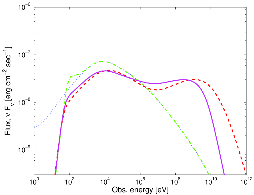
Figure 1.— Time averaged GRB prompt emission spectra obtained after 2 shells collision, characterized by low compactness parameter. Results are shown for $L=10^{52}$ erg, $\epsilon_{e}=\epsilon_{B}=10^{-0.5}$, $p=3$, $\Delta t=10^{-2}{\rm\ s}$ , $\Gamma=300$. The comoving compactness parameter is $l^{\prime}=2.5$. Dotted curve: cyclo- synchrotron emission only. Dash dotted curve: synchrotron emission and self absorption only. Dashed: synchrotron emission, synchrotron self absorption and Compton scattering. Solid: All processes included, including pair production and annihilation, but excluding proton acceleration. Luminosity distance $d_{L}=2\times 10^{28}$ and $z=1$ were assumed.

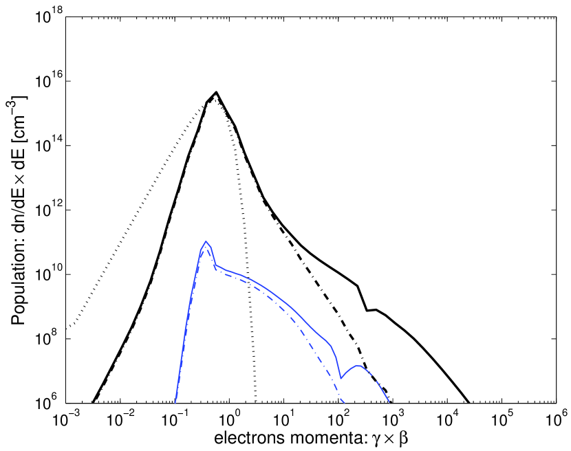
Figure 2.— Particle distribution at the end of the dynamical time. Thick: $\Delta t=10^{-4}{\rm\ s}$, $l^{\prime}=250$; Thin: $\Delta t=10^{-2}{\rm\ s}$, $l^{\prime}=2.5$. All other parameters are the same as in Figure 1. Solid: electron distribution, dash-dotted: positron distribution. The dotted line shows a Maxwellian distribution at temperature $\theta\equiv kT/m_{e}c^{2}=0.08$.

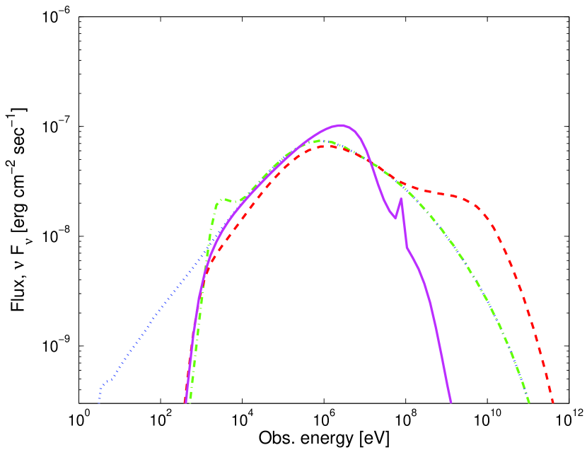
Figure 3.— Time averaged GRB prompt emission spectra obtained after 2 shells collision, characterized by high compactness parameter (not corrected for the high optical depth to Thompson scattering). Results are shown for $L=10^{52}$ erg, $\epsilon_{e}=\epsilon_{B}=10^{-0.5}$, $p=3$, $\Delta t=10^{-4}{\rm\ s}$ , $\Gamma=300$. The comoving compactness parameter is $l^{\prime}=250$. Dotted curve: cyclo- synchrotron emission only. Dash dotted curve: synchrotron emission and self absorption only. Dashed: synchrotron emission, synchrotron self absorption and Compton scattering. Solid: All processes included, including pair production and annihilation, but excluding proton acceleration. Luminosity distance $d_{L}=2\times 10^{28}$ and $z=1$ were assumed.

5. Summary & discussions

We described a time dependent numerical model which calculates emission of radiation from relativistic plasma, composed of homogeneous and isotropic distributions of electrons, positrons, protons and photons, and permeated by a time independent magnetic field. We assume the existence of a dissipation process, which produces energetic particles at constant rates. The particles interact via cyclo-synchrotron emission, synchrotron self absorption, inverse and direct Compton scattering, $e^{\pm}$ pair production and annihilation, and photo-meson interactions which produce energetic photons and positrons following the decay of energetic pions. Exact cross sections valid at all energies, including the Klein-Nishina suppression at high energies, are used in describing the physical processes. Exact spectra are used in describing cyclo-synchrotron emission, synchrotron self absorption, Compton scattering and pair production, and approximate spectra are used in the description of pair annihilation.

We explained in §3 our unique integration method, which overcomes the challenge of the many orders of magnitude difference in characteristic time scales. We presented the various integration techniques used for solving the kinetic equations describing the evolution of particle and photon distributions at all energy scales. By following directly the development of the rapid, high energy electro-magnetic cascades at each time step, we obtain the spectrum at high energies, up to $\geq 100\mbox{ TeV }$. Our method enables to follow the development of the spectrum created in the parameter space region of large compactness, where no analytic approximation is valid. This method also improves over previous ones by providing a more accurate treatment of photon emission and absorption in the presence of magnetic fields.

We have given several examples of numerical calculations in §4. In parameter space regions where analytical approximations are valid, our numerical results are in good agreement with analytic results. We have pointed out some significant discrepancies between the analytical approximations and the numerical calculation, and explained their origin. We presented examples of new results for parameter space regions where analytic approximations are not valid. We pointed out that our results are consistent with numerous observations, including observations that are inconsistent with the optically thin synchrotron-SSC model predictions. Further results of our study of GRB prompt emission and early afterglow emission can be found in Pe’er & Waxman (2004b, c).

The next generation high energy detectors, such as SWIFT and GLAST satellites, and the sub-TeV ground based Cerenkov detectors, such as MAGIC, HESS VERITAS and CANGAROO III are expected to increase the GRB prompt emission and early afterglow emission detection rate by an order of magnitude, to allow detection of $>\mbox{ GeV }$ emission from GRB’s, and to detect the high energy spectra of thousands of AGN’s at various distances. Thus, detailed numerical models, that are capable of producing accurate spectra over a wide energy scale, are necessary for analyzing and understanding the experimental data.

Appendix A Coulomb scattering

In the limit of relativistic particle scattering off cool thermal pair distribution ($\theta\ll 1$, $\gamma\gg 1$), the energy loss rate of the relativistic particle can be approximated by $d\gamma/dt\approx-3/2\sigma_{T}cn_{\pm}\ln\Lambda$, or $t_{ee}^{-1}\equiv-(1/\gamma)d\gamma/dt\approx 4\pi cr_{0}^{2}n_{\pm}\gamma^{-1}\ln\Lambda$ (Gould, 1975), where $n_{\pm}$ is the number density of the thermal pairs. The relevant value of the Coulomb logarithm $\Lambda$, is $\Lambda\approx\gamma^{1/2}m_{e}c^{2}/h\omega_{p}$, where $\omega_{p}=(4\pi n_{\pm}e^{2}/m_{e})^{1/2}$ is the plasma frequency.

Assuming that the pairs’ energy distribution is thermal, that their number density is $n_{\pm}\equiv fn_{p}$ where $n_{p}$ is the proton number density, and that $n_{p}\approx u_{int}/m_{p}c^{2}$ where $u_{int}$ is the internal energy density, comparing the Coulomb cooling time and the synchrotron cooling time, $t_{syn}=9m_{e}^{3}c^{5}/4q^{4}B^{2}\gamma$, using $B^{2}=8\pi\epsilon_{B}u_{int}$, gives

$${t_{syn}\over t_{ee}}={9\over 8}{m_{e}\over m_{p}}\frac{f\ln\Lambda}{\epsilon_{B}\gamma^{2}}\simeq\frac{1}{3\gamma^{2}}\,f_{1}\epsilon_{B,-0.5}^{-1},$$ (A1)

where typical values $f=10f_{1}$, and $\ln\Lambda\approx 20$ assumed. It is therefore concluded that for relativistic electrons, and for magnetic field not many orders of magnitude below equipartition, electrons lose their energy by synchrotron emission on a time scale much shorter than the energy loss time by Coulomb scattering. A more accurate approximation of $t_{ee}$ (Haug, 1988; Coppi & Blandford, 1990), does not change this result.

References

- Band et al. (1993) Band, D., et al. 1993, ApJ, 413, 281
- Baring & Braby (2004) Baring, M.G., & Braby, M.L. 2004, ApJ, 613, 460
- Bekefi (1966) Bekefi, G. 1966, Radiation Processes in Plasmas (New York: Wiley)
- Blumenthal & Gould (1970) Blumenthal, G.R., & Gould, R.J. 1970, Review of Modern Physics, 42, 237
- Bonometto & Rees (1971) Bonometto, S., & Rees, M.J. 1971, MNRAS, 152, 21
- Bötcher & Schlickeiser (1997) Bötcher, M., & Schlickeiser, R. 1997, A&A, 325, 866
- Burns & Lovelace (1982) Burns, M.L., & Lovelace, R.V.E. 1982, ApJ, 262, 87
- Coppi (1992) Coppi, P.S. 1992, MNRAS, 258, 657
- Coppi & Blandford (1990) Coppi, P.S., & Blandford, R.D. 1990, MNRAS, 245, 453
- Fabian et al. (1986) Fabian, A.C., Blandford, R.D., Guilbert, P.W., Phinney, E.S., & Cuellar, L. 1986, MNRAS, 221, 931
- Frontera et al. (2000) Frontera, F., et al. 2000, ApJS, 127, 59
- Ghirlanda, Celotti & Ghisellini (2003) Ghirlanda, G., Celotti, A., & Ghisellini, G. 2003, A&A, 406, 879
- Ghisellini, Guilbert & Svensson (1988) Ghisellini, G., Guilbert, P.W., & Svensson, R. 1988, ApJ, 334, L5