Phase mixing of shear Alfvén waves as a new mechanism for electron acceleration in collisionless, kinetic plasmas

Abstract

Particle-In-Cell (kinetic) simulations of shear Alfvén wave interaction with one dimensional, across the uniform magnetic field, density inhomogeneity (phase mixing) in collisionless plasma were performed for the first time. As a result a new electron acceleration mechanism is discovered. Progressive distortion of Alfvén wave front, due to the differences in local Alfvén speed, generates nearly parallel to the magnetic field electrostatic fields, which accelerate electrons via Landau damping. Surprisingly, amplitude decay law in the inhomogeneous regions, in the kinetic regime, is the same as in the MHD approximation described by Heyvaerts and Priest (1983).

Interaction of shear Alfvén waves (AWs) with plasma inhomogeneities is a topic of considerable importance both in astrophysical and laboratory plasmas. This is due to the fact both AWs and inhomogeneities often coexist in many of these physical systems. shear AWs are believed to be good candidates for plasma heating, energy and momentum transport. On the one hand, in many physical situations AWs are easily excitable and they are present in a number of astrophysical systems. On the other hand, these waves dissipate on shear viscosity as opposed to compressive fast and slow magnetosonic waves which dissipate on bulk viscosity. In astrophysical plasmas shear viscosity is extremely small as compared to bulk one. Hence, AWs are notoriously difficult to dissipate. One of the possibilities to improve AW dissipation is to introduce progressively collapsing spatial scales, $\delta l\to 0$, into the system (recall that the classical viscous and ohmic dissipation is $\propto\delta l^{-2}$). Heyvaerts and Priest have proposed (in astrophysical context) one such mechanism called AW phase mixing Heyvaerts and Priest (1983). It occurs when a linearly polarised shear AW propagates in the plasma with one dimensional, transverse to the uniform magnetic field density inhomogeneity. In such situation initially plane AW front is progressively distorted because of different Alfvén speeds across the field. This creates progressively strong gradients across the field (effectively in the inhomogeneous regions transverse scale collapses), and thus in the case of finite resistivity, dissipation is greatly enhanced. Thus, it is believed that phase mixing can provide substantial plasma heating. A significant amount of work has been done in the context of heating open magnetic structures in the solar corona Heyvaerts and Priest (1983); Nocera et al. (1986); Parker (1991); Nakariakov et al. (1997); Moortel et al. (2000); Botha et al. (2000); Tsiklauri et al. (2001); Hood et al. (2002); Tsiklauri and Nakariakov (2002); Tsiklauri et al. (2002, 2003). All phase mixing studies so far have been performed in the MHD approximation, however, since the transverse scales in the AW collapse progressively to zero, MHD approximation is inevitably violated, first, when the transverse scale approaches ion gyro-radius $r_{i}$ and then electron gyro-radius $r_{e}$. Thus, we proposed to study phase mixing effect in the kinetic regime, i.e. we go beyond MHD approximation. As a result we discovered new mechanism of electron acceleration due to wave-particle interactions which has important implications for various space and laboratory plasmas, e.g. coronal heating problem and acceleration of solar wind.

We used 2D3V, the fully relativistic, electromagnetic, particle-in-cell (PIC) code with MPI parallelisation, modified from 3D3V TRISTAN code Buneman (1993, p.67). The system size is $L_{x}=5000\Delta$ and $L_{y}=200\Delta$, where $\Delta(=1.0)$ is the grid size. The periodic boundary conditions for $x$- and $y$-directions are imposed on particles and fields. There are about 478 million electrons and ions in the simulation. The average number of particles per cell is 100 in low density regions (see below). Thermal velocity of electrons is $v_{th,e}=0.1c$ and for ions is $v_{th,i}=0.025c$. The ion to electron mass ratio is $m_{i}/m_{e}=16$. The time step is $\omega_{pe}\Delta t=0.05$. Here $\omega_{pe}$ is the electron plasma frequency. The Debye length is $v_{th,e}/\omega_{pe}=1.0$. The electron skin depth is $c/\omega_{pe}=10\Delta$, while the ion skin depth is $c/\omega_{pi}=40\Delta$. Here $\omega_{pi}$ is the ion plasma frequency. The electron Larmor radius is $v_{th,e}/\omega_{ce}=1.0\Delta$, while the same for ions is $v_{th,i}/\omega_{ci}=4.0\Delta$. The external uniform magnetic field, $B_{0}$, is in the $x$-direction and the initial electric field is zero. The ratio of electron cyclotron frequency to electron plasma frequency is $\omega_{ce}/\omega_{pe}=1.0$, while the same for ions is $\omega_{ci}/\omega_{pi}=0.25$. The latter ratio is essentially $V_{A}/c$ – the Alfvén speed. Plasma $\beta=2(\omega_{pe}/\omega_{ce})^{2}(v_{th,e}/c)^{2}=0.02$. Here all plasma parameters are quoted far away from the density inhomogeneity region. The dimensionless (normalised to some reference constant value of $n_{0}$) ion and electron density inhomogeneity is described by

$${n_{i}(y)}={n_{e}(y)}=1+3\exp\left[-\left({(y-100\Delta)}/{(50\Delta)}\right)^{6}\right]\equiv F(y).$$ (1)

This means that in the central region (across $y$-direction) density is smoothly enhanced by a factor of 4, and there are strong density gradients of width of about ${50\Delta}$ around the points $y=51.5\Delta$ and $y=148.5\Delta$. The background temperature of ions and electrons, and their thermal velocities are varied accordingly

$${T_{i}(y)}/{T_{0}}={T_{e}(y)}/{T_{0}}=F(y)^{-1},$$ (2)

$${v_{th,i}}/{v_{i0}}={v_{th,e}}/{v_{e0}}=F(y)^{-1/2},$$ (3)

such that the thermal pressure remains constant. Since the background magnetic field along $x$-coordinate is also constant, the total pressure remains constant too. Then we impose current of the following form

$${\partial_{t}E_{y}}=-J_{0}\sin(\omega_{d}t)\left(1-\exp\left[-(t/t_{0})^{2}\right]\right),$$ (4)

$${\partial_{t}E_{z}}=-J_{0}\cos(\omega_{d}t)\left(1-\exp\left[-(t/t_{0})^{2}\right]\right).$$ (5)

Here $\omega_{d}$ is the driving frequency which was fixed at $\omega_{d}=0.3\omega_{ci}$, which ensures that no significant ion-cyclotron damping is present. Also, $\partial_{t}$ denotes time derivative. $t_{0}$ is the onset time of the driver, which was fixed at $50/\omega_{pe}$ or $3.125/\omega_{ci}$. This means that the driver onset time is about 3 ion-cyclotron periods. Imposing such current on the system results in the generation of left circularly polarised shear AW, which is driven at the left boundary of simulation box and has a width of $1\Delta$. Initial amplitude of the current is such that relative AW amplitude is about 5 % of the background in the low density regions, thus the simulation is weakly non-linear.

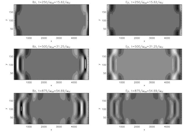
Because of no initial (perpendicular to the external magnetic field) velocity excitation was imposed in addition to the above specified currents (cf. Tsiklauri and Nakariakov (2002)), the excited (driven) at the left boundary circularly polarised AW is split into two circularly polarised AWs that travel in opposite directions. The dynamics of these waves is shown in Fig.1 where we show three snapshots of the evolution. Typical simulation, till the last snapshot shown in the figure, takes about 8 days on the parallel 32 dual 2.4 GHz Xeon processors. It can be seen from the figure that because of the periodic boundary conditions circularly polarised AW that was travelling to the left has reappeared from the right side of the simulation box ($t=15.62/\omega_{ci}$). Then the dynamics of the AW ($B_{z},E_{y}$) progresses in a similar manner as in MHD, i.e. it phase mixes Heyvaerts and Priest (1983). In other words middle region (in $y$-coordinate) travels slower because of the density enhancement (note that $V_{A}(y)\propto 1/\sqrt{n_{i}(y)}$). This obviously causes distortion of initially plane wave front and the creation of strong gradients in the regions around $y=50$ and $150$. In MHD approximation, in the case of finite resistivity $\eta$, in these regions AW is strongly dissipated due to enhanced viscous and ohmic dissipation. This effectively means that the outer and inner parts of the travelling AW are detached from each other and propagate independently. This is why the effect is called phase mixing – after long time, in the case of developed phase mixing, phases in the wave front become effectively uncorrelated. A priori it was not clear what to expect from our PIC simulation because it was performed for the first time. The code is collisionless and there are no sources of dissipation in it (apart from possibility of wave-particle interactions). It is evident from Fig.1 that at later stages ($t=54.69/\omega_{ci}$) AW front is strongly damped in the strong density gradient regions. This immediately rises a question of where AW energy went? The answer lies in Fig. 2, where we plot $E_{x}$ longitudinal electrostatic field, and electron phase space ($V_{x}/c$ vs. $x$) for the different times (note, that in order to reduce figure size, only electrons with $V_{x}>0.15c$ were plotted). In the regions around $y=50$ and $150$ for later times significant electrostatic field is generated. This is the consequence of stretching of AW front in those regions because of difference in local Alfvén speed. In the right column of this figure we see that exactly in those regions where $E_{x}$ is generated, the electrons are accelerated in large numbers. Thus, we conclude that energy of the phase mixed AW goes into acceleration of electrons. In fact line plots of $E_{x}$ show that this electrostatic field is strongly damped. i.e. energy is channelled to electrons via Landau damping.

The next piece of evidence comes from looking at the distribution function of electrons before and after the phase mixing took place. In Fig.3 we plot distribution function of electrons at $t=0$ and $t=54.69/\omega_{ci}$. Note that even at $t=0$ the distribution function does not look as purely Maxwellian because of the fact that temperature varies across $y-$coordinate (to keep total pressure constant) and the graph is produced for the entire simulation domain. There is also a substantial difference at $t=54.69/\omega_{ci}$ to its original form because of the aforementioned electron acceleration. We see that the number of electrons having velocities $V_{x}=\pm(0.1-0.3)c$ is increased. Note that the acceleration of electrons takes place mostly along the external magnetic field (along $x$-coordinate). No electron acceleration occurs in $V_{y}$ or $V_{z}$ (not plotted here).

The next step is to check whether the increase in electron velocities comes from the resonant wave particle interactions. For this purpose in Fig. 4 we plot two snapshots of Alfvén wave $B_{z}(x,y=148)$ components at instances $t=54.69/\omega_{ci}$ (solid line) and $t=46.87/\omega_{ci}$ (dotted line). The distance between the two upper leftmost peaks (which is the distance travelled by the wave in time between the snapshots) is about $\delta L=150\Delta=15(c/\omega_{pe})$. Time difference between the snapshots is $\delta t=7.82/\omega_{ci}$. Thus, measured AW speed at the point of the strongest density gradient ($y=148$) is $V_{A}^{M}=\delta L/\delta t=0.12c$. Now we can also work out the Alfvén speed. In the homogeneous low density region the Alfvén speed was set to be $V_{A}(\infty)=0.25c$. From Eq.(1) it follows that for $y=148$ density is increased by a factor of $2.37$ which means that the Alfvén speed at this position is $V_{A}(148)=0.25/\sqrt{2.37}c=0.16c$. The measured and calculated Alfvén speeds in the inhomogeneous region do not coincide. This can be attributed to the fact that in the inhomogeneous regions (where electron acceleration takes place) because of momentum conservation AW front is decelerated as it passes on energy and momentum to the electrons. However, this may be not the case if wave-particle interactions play the same role as dissipation in the MHD: Then wave-particle interactions would result only in the decrease of the AW amplitude (dissipation) not in its deceleration. If we compare these values to Fig.3, we deduce that these are the velocities $>0.12c$ above which electron numbers with higher velocities are greatly increased. This deviation peaks at about $0.25c$ which in fact corresponds to the Alfvén speed in the lower density regions. This can be explained by the fact the electron acceleration takes place in wide regions (cf. Fig. 2) along and around $y=148$ (and $y=51$) – thus the spread in the accelerated velocities.

In Fig.4 we also plot a visual fit curve (dashed line) in order to quantify the amplitude decay law for the AW (at $t=54.69/\omega_{ci}$) in the strongest density inhomogeneity region. The fitted (dashed) cure is represented by $0.056\exp\left[-\left({x}/{1250}\right)^{3}\right]$. There is an astonishing similarity of this fit with the MHD approximation results. Authors of Ref. Heyvaerts and Priest (1983) found that for large times (developed phase mixing), in the case of harmonic driver, the amplitude decay law is given by $\propto\exp\left[-\left(\frac{\eta\omega^{2}V_{A}^{\prime 2}}{6V_{A}^{5}}\right)x^{3}\right]$ which is much faster than the usual resistivity dissipation $\propto\exp(-\eta x)$. Here $V_{A}^{\prime}$ is the derivative of the Alfvén speed with respect to $y$-coordinate. The most intriguing fact is that even in the kinetic approximation the same $\propto\exp(-Ax^{3})$ law holds as in the MHD. In the MHD a finite resistivity and Alfvén speed non-uniformity are responsible for the enhanced dissipation via phase mixing mechanism. In our PIC simulations (kinetic phase mixing), however, we do not have dissipation and collisions (dissipation). Thus, in our case wave-particle interactions play the same role as resistivity $\eta$ in the MHD phase mixing. It should be noted that no significant AW dissipation was found away from the density inhomogeneity regions. This has the same explanation as in the case of MHD – it is the regions of density of inhomogeneities ($V_{A}^{\prime}\not=0$) where the dissipation is greatly enhanced, while in the regions where $V_{A}^{\prime}=0$ there is no substantial dissipation (apart from classical $\propto\exp(-\eta x)$ one). In MHD approximation aforementioned amplitude decay law is derived from the diffusion equation, to which MHD equations reduce to for large times (developed phase mixing). It seems that kinetic description leads to the same type of diffusion equation. It is unclear although, at this stage, what physical quantity would play role of resistivity $\eta$ (from the MHD approximation) in the kinetic regime.

It is worthwhile to mention that in MHD approximation authors of Refs. Hood et al. (2002); Tsiklauri et al. (2003) showed that in the case of localised Alfvén pulses, Heyvaerts and Priest’s amplitude decay formula $\propto\exp(-Ax^{3})$ (which is true for harmonic AWs) is replaced by the power law $B_{z}\propto x^{-3/2}$. A natural next step forward would be to check whether in the case of localised Alfvén pulses the same power law holds in the kinetic regime.

Finally we would like to mention that after this study was complete we became aware of study by Vasquez and Hollweg (2004), who used hybrid code (electrons treated as neutralising fluid, while ion kinetics is retained) as opposed to our (fully kinetic) PIC code, to simulate resonant absorption. They found that a planar (body) Alfvén wave propagating at less than $90^{\circ}$ to a background gradient has field lines which lose wave energy to another set of field lines by cross-field transport. Further, Vasquez (2004) found that when perpendicular scales of order 10 proton inertial lengths ($10c/\omega_{pi}$) develop from wave refraction in the vicinity of the resonant field lines, a non-propagating density fluctuation begins to grow to large amplitudes. This saturates by exciting highly oblique, compressive, and low-frequency waves which dissipate and heat protons. These processes lead to a faster development of small scales across the magnetic field, i.e. this is ultimately related to the phase mixing mechanism, studied here. Continuing this argument we would like make clear distinction between the effects of phase mixing and resonant absorption of the shear Alfvén waves. Historically, there was some confusion in use of there terms. In fact, earlier studies which were performed in the context of laboratory plasmas, e.g. Ref. Hasegawa and Chen (1974) who proposed (quote) ”the heating of collisionless plasma by utilising a spatial phase mixing by shear Alfvén wave resonance and discussed potential applications to toroidal plasma” used term phase mixing to discuss the physical effect which in reality was the resonant absorption. In their later works, Hasegawa and Chen (1975) and Hasegawa and Chen (1976), when they treated the same problem in the kinetic approximation (note that Hasegawa and Chen (1974) used MHD approach) the authors avoided further use of term phase mixing and instead they talked about linear mode conversion of shear Alfvén wave into kinetic Alfvén wave near the resonance $\omega^{2}=k_{\parallel}^{2}V_{A}(x)$ (in their geometry the inhomogeneity was across the $x$-axis). In the kinetic approximation Hasegawa and Chen (1975) and Hasegawa and Chen (1976) found a number of interesting effects including:

(i) They established that near the resonance initial shear Alfvén wave is linearly converted into kinetic Alfvén wave (which is the Alfvén wave modified by the finite ion Larmor radius and electron inertia) that propagates almost parallel to the magnetic field into the higher density side. Inclusion of the finite ion Larmor radius and electron inertia removes the logarithmic singularity present in the MHD resonant absorption which exists because in MHD shear Alfvén wave cannot propagate across the magnetic field. Physically this means that finite ion Larmor radius prevents ting ions to magnetic field lines and thus allows propagation across the field. The electron inertia eliminates singularity in the same fashion but on different, $r_{i}\sqrt{T_{e}/T_{i}}$, spatial scale (here $r_{i}$ ion gyro-radius).

(ii) They also found that in collionless regime (which is applicable to our case) dissipation of the (mode converted) kinetic Alfvén wave is through Landau damping of parallel electric fields both by electrons and ions. However, in the low plasma $\beta$ regime (which is also applicable to our case $\beta=2(\omega_{pe}/\omega_{ce})^{2}(v_{th,e}/c)^{2}=0.02$) they showed that only electrons are heated (accelerated), but not the ions. In our numerical simulations we see similar behaviour: i.e. preferential acceleration of electrons (cf. Tsiklauri et al. (2005)). In spite of this similarity, however, one should make clear distinction between (a) phase mixing which essentially is a result of enhanced, due to plasma inhomogeneity, collisional viscous and ohmic dissipation and (b) resonant absorption which can operate in the collisionless regime as a result of generation of kinetic Alfvén wave in the resonant layer, which subsequently decays via Landau damping preferentially accelerating electrons in the low $\beta$ regime.

(iii) They also showed that in the kinetic regime the total absorption rate is approximately the same as in the MHD. Our simulations seem to produce similar results. We cannot comment quantitatively on this occasion, but at least the spatial from of the amplitude decay ($\propto\exp(-Ax^{3})$) is similar in both cases.

Resuming aforesaid, we conjecture that the generated nearly parallel electrostatic fields found in our numerical simulations are due to the generation of kinetic Alfvén waves that are created through interaction of initial shear Alfvén waves with plasma density inhomogeneity, in a similar fashion as in resonant absorption described above. Further theoretical study is thus needed to provide solid theoretical basis for interpretation of our numerical simulation results and to test the above conjecture.

Figure 1: Contour (intensity) plots of phase mixed Alfvén wave $B_{z}$ and $E_{y}$ components at instants: $t=(15.62,31.25,54.69)/\omega_{ci}$. Excitation source is at the left boundary. Because of periodic boundary conditions, left-propagating AW re-appears from the right side of the simulation box. Note how AW is progressively stretched because of differences in local Alfvén speed.

Figure 2: Left column: contour plots of generated nearly parallel to the external magnetic field electrostatic field $E_{x}$ at instants: $t=(15.62,31.25,54.69)/\omega_{ci}$. Right column: $x$-component of electron phase space at the same times. Note, that in order to reduce figure size, only electrons with $V_{x}>0.15c$ were plotted.

Figure 3: The distribution function of electrons at $t=0$ (dotted curve) and $t=54.69/\omega_{ci}$ (solid curve).

Figure 4: Two snapshots of Alfvén wave $B_{z}(x,y=148)$ component at instants $t=54.69/\omega_{ci}$ (solid line) and $t=46.87/\omega_{ci}$ (dotted line). Dashed line represents fit $0.056\exp\left[-\left({x}/{1250}\right)^{3}\right]$.