Novel Geometrical Models of Relativistic Stars.
I. The General Scheme

Abstract

In a series of articles we describe a novel class of geometrical models of relativistic stars. Our approach to the static spherically symmetric solutions of Einstein equations is based on a careful physical analysis of radial gauge conditions. It brings us to a two parameter family of relativistic stars without stiff functional dependence between the stelar radius and stelar mass. It turns out that within this family there do exist relativistic stars with arbitrary large mass, which are to have arbitrary small radius and arbitrary small luminosity. In addition, point particle idealization, as a limiting case of bodies with finite dimension, becomes possible in GR, much like in Newton gravity.

PACS number(s): 04.20.Cv, 04.20.Jb, 04.20.Dw

I Introduction

Today the theory of relativistic stars is a well developed branch of relativistic physics with many observational confirmations. It is based on general relativity (GR), as a relativistic theory of gravity, on quantum statistical physics, as a theory of many-particle systems, and on the latest achievements of the standard model (SM), as a modern theory of matter constituents. (See the books books and the large amount of references therein.)

The role of quantum statistics of the Fermi gas in theory of neutron stars has been clarified in the pioneering articles by Chandrasekhar and Landau CL on the non-relativistic ground of Newton gravity. For this purpose was used the analogy with the theory of white dwarfs Chandra .

The beginning of the relativistic stelar theory can be found in the pioneering articles by Schwarzschild Schwarzschild , Tolmen, and Openheimer$\&$Volkov (TOV) TOV , an important further developments – in developments .

After the appearance of these articles the relativistic theory of gravity of spherically symmetric static stars is widely accepted as a well established issue. The further developments are related with various considerations of the physics of stelar matter and with a search of more realistic equations of state (EOS) of this matter for different types of stars. This line of investigation is continuously followed up to now, see EOS and the references therein.

In spite of general success of the relativistic theory of stars, at present it can not be considered as a complete established scientific area in its final form. (See, for example, the recent review articles ns and the references therein.)

Some difficulties in the explanation of the properties of very dense stars, like neutron stars or eventual quark ones, are suspected nsDiff and need a proper explanation. The currently used approach of continuous modification of EOS already brought us to EOS, which are extension of known physical laws onto domain where we have no experimental information. Therefore some additional, more or less arbitrary assumptions are needed.

To some extend, a similar situation we may observe in the theory of white dwarfs, see, for example, WD and the references therein, as well as some additional comments in Section V, B.

Unfortunately, we still do not have a complete set of observational data for a direct confrontation of the present-days relativistic theory with astrophysical observations. In particular we do not have precise observational data both for the mass and the radii of a given neutron star, we do not know the precise upper limit of neutron star masses, e.t.c.

The existence of such universal upper limit is a basic prediction of the modern relativistic theory of stars, but the theory is not able to give a definite predictions for the corresponding value, due to the uncertainties in EOS. As a result, all observed massive compact dark objects with gravitational mass $m_{*}\gtrsim(5-10)\times m_{\odot}$ are automatically interpreted as a candidates for black holes, despite of the fact that there still do not exist undisputable direct observational evidences for existence of such exotic objects with their non-avoidable attribute - the event horizon BH .

The fast development of this scientific domain calls for a further investigation of different aspects of the general theory, including its basic assumptions.

In the present series of articles we will not consider the EOS problem, nor the complicated dynamical problems of rotating stars, or stelar oscillations. Here we will reconsider some basic features of relativistic theory of gravity when applied to the study of stelar physics in the simplest static spherically symmetric case. We shall show that there exist new classes of models for relativistic stars, thus enlarging essentially the general theoretical scheme. We hope that the new relativistic models may lead to a better understanding of the real astrophysical observations.

Here we utilize a new approach to the spherically symmetric static solutions to Einstein equations (EE), based on careful analysis of the radial gauge. Recently this approach brought into the world a new two-parameter family of solutions of EE with a massive point source and some unexpected physical consequences, see F03 . One of them is that in the point particle problem the global analytical properties of the solutions of EE in complex plain of the radial variable are fixing this variable in a unique way, together with the corresponding boundary conditions. Similar phenomenon is well known in the theory of analytical functions: they are unambiguously defined by their singular points in complex domain.

In mathematical sense this way were derived the fundamental static spherically symmetric solutions of EE. These solutions are analogous to the fundamental solutions of classical Poison equation with point source. Here we are extending this approach to the theory of relativistic stars.

II The Physical Consequences of the Choice of Radial Gauge in the Stelar Problem

The EE determine the solution of a given physical problem up to four arbitrary functions, i.e., up to a choice of coordinates. This reflects the well known fact that GR is a gauge theory. According to the standard textbooks books , the fixing of the gauge in GR in a holonomic frame is represented by a proper choice of the quantities

$$\bar{\Gamma}_{\mu}\!=\!-{{1}\over{\sqrt{|g|}}}g_{\mu\nu}\partial_{\lambda}\left(\sqrt{|g|}g^{\lambda\nu}\right),$$ (II.1)

which emerge when one expresses the 4D d’Alembert operator in the form $g^{\mu\nu}\nabla_{\mu}\nabla_{\nu}=g^{\mu\nu}\left(\partial_{\mu}\partial_{\nu}-\bar{\Gamma}_{\mu}\partial_{\nu}\right)$. Unfortunately, up to now physically reasonable principles for the choice of the gauge in GR are not known. Moreover, at present many of the relativists are thinking that this is not a physically essential GR problem.

We shall call the change of the gauge fixing expressions (II.1), without any preliminary conditions on the analytical behavior of the used functions, a gauge transformations in a broad sense. This way we essentially expand the class of the gauge transformations, we intend to discuss, looking for a physically meaningful choice of the gauge conditions (II.1).

In the static spherically symmetric problems the structure of the space-time is $\mathbb{M}^{(1,3)}=T_{t}(1)\times\mathbb{M}^{(1)}_{r}\times SO(3)$. There exists unambiguous choice of the global time $t$ on the 1D time-translations group $T_{t}(1)$ and of the angle variables $\theta$, $\phi$ – on the $SO(3)$ group space. These variables are unambiguously fixed by symmetry reasons. In proper units (in which the velocity of light is $c=1$) this choice yields the familiar form of the space-time interval:

$$ds^{2}=g_{tt}(r)\,dt^{2}\!+g_{rr}(r)\,dr^{2}\!-\!\rho(r)^{2}(d\theta^{2}\!+\!\sin^{2}\theta\,d\phi^{2})\hskip 8.5359pt$$ (II.2)

with unknown functions $g_{tt}(r)>0,\,g_{rr}(r)<0,\,\rho(r)$.

Thus the form of three of the gauge fixing coefficients (II.1):  $\bar{\Gamma}_{t}\!=\!0,\,\,\bar{\Gamma}_{\theta}\!=-\!\cot\theta,\,\,\bar{\Gamma}_{\phi}\!=\!0$ is fixed by symmetry reasons, but the quantity

$$\bar{\Gamma}_{r}\!=\left(\!\ln\left({\sqrt{-g_{rr}}\over{\sqrt{g_{tt}}\,\rho^{2}}}\right)\!\right)^{\prime}\!=\!\left(\!\ln\left({\rho^{\prime}{\sqrt{-g_{\rho\rho}}}\over{\rho^{2}\,\sqrt{g_{tt}}}}\right)\!\right)^{\prime},$$ (II.3)

and, equivalently, the function $\rho(r)$ are still not fixed. Here and further on, the prime denotes differentiation with respect to the variable $r$.

The physical and the geometrical meaning of the radial coordinate $r$ is not defined by symmetry reasons and is unknown a priori Eddington ; F03 . The only clear thing is that its value $r=0$ corresponds to the center of $SO(3)$ symmetry. In the case of relativistic stars with regular distribution of matter this 3D-space point is the physical center of the star, where the mass $m(r)$, surrounded by a sphere with coordinate radius $r=0$, is $m(0)=0$.

We shall use this physical property of the mass as a definition of the star’s center $C$, because it does not depend on the choice of the radial variable $r$. Thus the mass $m$ can be used to find the geometrical place at which the proper radial variable $r$ must equals zero. This is the main specific feature of our approach to the theory of the relativistic stars.

In contrast to the radial variable $r$, the quantity $\rho$ has a clear geometrical and physical meaning: $\rho$ defines the area $A_{\rho}=4\pi\rho^{2}$ of a centered at the center $C$ sphere with ”area radius” $\rho$. From physical point of view one can refer to this quantity as ”a luminosity variable“ (or ”a luminosity radius”), because the luminosity of distant physical objects is reciprocal to $A_{\rho}$. In other words, the variable $\rho$ describes the spherically symmetric spreading of energy of any kind.

We refer to the choice of the function $\rho(r)$ as a choice of radial gauge in a broad sense F03 , allowing, in general, singular changes of the variable $r$. We call the freedom of choice of the function $\rho(r)$ ”a rho-gauge freedom” in a broad sense, and any definite choice of function $\rho(r)$ – ”a rho-gauge fixing”.

At first glance the fixing of the function $\rho(r)$ seems to be rather arbitrary and without any physical significance.

From geometrical point of view the choice of the radial gauge defines an imbedding of the 1D quotient space $\mathbb{M}^{(1)}_{r}\!=\!\left(\mathbb{M}^{(1,3)}/T_{t}(1)\right)\!/\!SO(3)$ into the space-time $\mathbb{M}^{(1,3)}$.

For fixing of this additional mathematical structure one needs some physical conditions like boundary conditions, or conditions for fixing of the number and the character of singular points of the solution of EE in the whole complex domain. This was demonstrated in F03 for the case of fundamental singular solutions of EE with massive point source. These additional conditions play an essential role in the problem, because they are determining the global analytical properties of the solutions. Actually they define the very manifold $\mathbb{M}^{(1,3)}$.

The EE are holomorphic ones and their solutions must be studied in the whole complex domain of corresponding variables. The very EE do determine only the local structure of $\mathbb{M}^{(1,3)}$. In our case the change of the function $\rho(r)$ will be not a simple change of the labels of space-time points, if it changes the additional conditions, which fix the analytical properties of the manifold $\mathbb{M}^{(1,3)}$ in the whole complex domain F03 .

Our present consideration illustrates this important juncture on the more physical example of solar models:

It is obvious that physical results of any theory must not depend on the choice of the variables. In particular, these results must be invariant under changes of coordinates. This requirement is a basic principle not only in GR. It is fulfilled for any already fixed mathematical problem.

Nevertheless, the change of the interpretation of the variables may change the very mathematical problem and some physical results, because we are using the variables according to their interpretation. For example, if we are considering the luminosity variable $\rho$ as a radial variable of the problem, it seems natural to put the center of the star at the point $\rho=0$. In general, we may obtain a physically different stelar model, if we are considering another variable $r$ as a radial one: in this case we shall place the star’s center at a different geometrical point $r=0$, which now seems to be the natural position of the physical center $C$. The relation between these two geometrical ”points” and between the corresponding stelar models strongly depends on the choice of the function $\rho(r)$, i.e. on the radial gauge.

Thus, applying the same physical requirements, like

$$m|_{\hbox{\small at the center}\,\,C}=0,$$ (II.4)

in different ”natural” variables, we arrive at different physical models, because we are solving EE under different boundary conditions. One has to find a theoretical or an experimental reasons to resolve this essential ambiguity, or one has to accept it as an non-avoidable component of the theory, recovering its physical meaning and its proper usage.

The physical center $C$ of the star is placed at the point $r=0$ by definition. To what value of the luminosity variable $\rho_{C}=\rho(0)$ corresponds the real position of the center $C$ is not known a priori. This depends strongly on the choice of the rho-gauge function $\rho(r)$. One can not exclude such nonstandard behavior of the physically reasonable gauge function $\rho(r)$, which leads to some value $\rho_{C}>0$ F03 .

This very interesting novel possibility emerges in curved space-times due to their unusual geometrical properties and is not supported by our Euclidean experience. It will be the main subject of study in the present series of articles. Such possibility was discovered at first in the original pioneering article by Schwarzschild Schwarzschild1 and discussed by Brillouin Brillouin , but at present it is widely ignored. A physical necessity of considering values of the $\rho$-variable, not less the Schwarzschild radius, was stressed by Dirac Dirac , too.

The present-days standard theory of relativistic stars is based on the Hilbert radial gauge (HG): $\rho(r)\equiv r$. In this gauge the center of the star is placed at the point $\rho_{C}=\rho(0)=0$. This rather arbitrary additional condition was at first utilized by Schwarzschild in his simple model of incompressible stars Schwarzschild . There he had used formal mathematical reasons to be able to fix this way one of the integration constants. Actually he had postulated the global geometrical properties of the stelar center $C$ in curved space-time, adopting the ones, which take place in the non-relativistic Euclidean case.

The local reason seems to be Eq. (II.4), which entails asymptotically flat 3D metric in a small enough vicinity of the stelar center $C$. According to GR, the spherically symmetric distribution of the masses outside this vicinity does not influence the flat geometry around $C$.

Nevertheless, one has to take into account that there is no guaranty that starting from some luminosity $L_{*}\rightleftarrows\rho_{*}$ at the stelar surface, and going trough the curved 3D space back to the center $C$, defined by Eq. (II.4), we will reach the value $\rho_{C}=0$. This is what we mean by ”global” property of center $C$. This property of the center $C$ depends on properties of the interior solution of stelar problem in the whole interior domain. From point of view of TOV system of differential equations, such property of the center $C$ depends on the global properties of the inner solution.

The assumption $\rho_{C}=0$ has a strong influence on the further development of the theory of relativistic stars. In particular, it forces one to impose a regularity condition at the point $\rho=0$ both on the matter distribution and on the solutions of EE. As a result, one uses only a very specific solutions of TOV equations for relativistic stars books –ns . These solutions form a set of zero measure in the variety of all solutions of the problem. Thus one is forced to ignore the vast majority of the solutions, which are of general type and do not obey the regularity condition at the point $\rho=0$.

The novel solutions of EE for massive point particle, discovered in F03 , raise a new understanding of the role of the luminosity variable $\rho$. Here we shall show that in the relativistic theory of stars the same approach allows a consideration of all solutions of the TOV equations in a physically meaningful way. This way we essentially enrich the relativistic theory of stars.

An extremely important consequence of our more wide treatment of stelar models is the existence of relativistic stars with arbitrary large mass, and, at the same time, with arbitrary small geometric radius and arbitrary small luminosity. This unexpected possibility will be mathematically proved for incompressible relativistic stars in a subsequent article.

The strong nonlinearity both of the differential equations and the boundary conditions may yield, in general, several different classes of new solutions. This resembles the real situation, illustrated by the well known Hertzsprung-Russell diagram for stars in Nature HR .

Because of presence of the additional parameter $\rho_{C}$ in the general solutions of TOV equations, the total mass of the star $m_{*}$ is not a function only of its coordinate radius $r_{*}$ (or geometrical radius $R_{*}$, or luminosity radius $\rho_{*}$) and may vary independently of it. Due to this property, our approach gives for the first time a possibility to consider the point particles in GR as a limiting case of a body with finite dimension, much like in the Newton theory of gravity. This important new feature will be described in another subsequent article.

The considerations in this first of series of articles has a preliminary character, setting in a new way the relativistic theory of gravity in the stelar physics. This article does not aim a construction of a specific models of relativistic stars. Here we give only the new general scheme for such considerations. Due to technical reasons we describe specific models of relativistic stars with different EOS and other further developments elsewhere.

III Solution of the Extended TOV System in Hilbert Gauge

The luminosity variable $\rho$ gives a very convenient description of stelar structure in real domain. The use of this variable ensures a local radial-gage-invariance of the approach to solution of this problem. Therefore, keeping the traditions, we shall work in this Section in HG. In our consideration the values $\rho<\rho_{C}$ have no physical meaning. The values $\rho\in[\rho_{C},\rho_{*}]$ describe the inner domain and the values $\rho\in(\rho_{*},\infty)$ correspond to the exterior vacuum domain outside the star.

Then the inner metric (II.2) for a static spherically symmetric star is defined by the metric components

$$g_{tt}(\rho;\rho_{*},\rho_{C})\!=\!e^{2\varphi(\rho;\rho_{*},\rho_{C})},$$

$$g_{\rho\rho}(\rho,;\rho_{*},\rho_{C})\!=\!{-1\over{1\!-\!2m(\rho;\rho_{*},\rho_{C})/\rho}}.$$ (III.1)

Here and further on we are using units $c=G_{N}=1$.

The mass $m(\rho;\rho_{*},\rho_{C})$, surrounded by a sphere with a luminosity radius $\rho$, obeys the first TOV equation:

$${{dm}\over{d\rho}}=4\pi\varepsilon\rho^{2}>0,$$ (III.2)

supplemented by the boundary conditions

$$m(\rho_{C};\rho_{*},\rho_{C})=0,\,\,\,\,m(\rho_{*};\rho_{*},\rho_{C})=m(\rho_{*},\rho_{C}).$$ (III.3)

The first condition is the definition of the physical center $C$ of the star, placed at a position with unknown value of the luminosity variable $\rho_{C}\geq 0$. The second one defines the total mass of the star $m(\rho_{*},\rho_{C})$, obtained using the unknown value of the luminosity variable $\rho_{*}\geq\rho_{C}$ at the edge of the star.

As a consequence of Eq.(III.1) and (III.2) we obtain for any admissible value of $\rho_{C}$ the relation $-g_{\rho\rho}(\rho_{C};\rho_{*},\rho_{C})=1$.

The pressure $p(\rho;\rho_{*},\rho_{C})$ obeys the equation

$${{dp}\over{d\rho}}=-{{(p+\varepsilon)(m+4\pi\rho^{3}p)}\over{\rho(\rho-2m)}}<0,$$ (III.4)

where $\varepsilon(\rho;\rho_{*},\rho_{c})$ is the energy density. The boundary conditions for this equation are:

$$p(\rho_{C};\rho_{*},\rho_{C})=p_{C}(\rho_{*},\rho_{C}),\,\,\,\,p(\rho_{*};\rho_{*},\rho_{C})=0.$$ (III.5)

Here $p_{C}$ is the pressure at the star center $C$. The second condition defines the physical edge of the star.

One has to extend the above TOV system adding the equation for the proper mass $m_{0}(\rho;\rho_{*},\rho_{c})$ of the star in the sphere with luminosity radius $\rho$:

$${{dm_{0}}\over{d\rho}}=4\pi\varepsilon\rho^{2}\sqrt{-g_{\rho\rho}}>0,$$ (III.6)

together with the boundary conditions

$$m_{0}(\rho_{C};\rho_{*},\rho_{C})=0,\,\,\,\,m_{0}(\rho_{*};\rho_{*},\rho_{C})=m_{0}(\rho_{*},\rho_{C}).\hskip 14.22636pt$$ (III.7)

and the equation for the gravitational potential $\varphi(\rho;\rho_{*},\rho_{C})$:

$${{d\varphi}\over{d\rho}}={{m+4\pi\rho^{3}p}\over{\rho(\rho-2m)}}>0,$$ (III.8)

together with the boundary conditions

$$\varphi(\rho_{C};\!\rho_{*},\rho_{C})\!=\!\varphi_{C}(\rho_{*},\rho_{C}),\,\varphi(\rho_{*};\!\rho_{*},\rho_{C})\!=\!\varphi(\rho_{*},\rho_{C}).\hskip 14.22636pt$$ (III.9)

To have a closed system of mathematical equations one has to add the EOS. It can be defined in different equivalent forms. The most convenient for our general considerations is the following one:

$$\varepsilon=\varepsilon(p).$$ (III.10)

It is useful to introduce, too, the quantity

$$w=p/\varepsilon.$$ (III.11)

As a result of our consideration we see that the description of stelar structure leads to a correct mathematical boundary problem with unknown ends $\rho_{C}$ and $\rho_{*}$.

IV Solution of a Cauchy Problem as a Method of Solution of the Stellar Boundary Problem

As we have seen in the previous Section, the stelar structure is determined by solution of the boundary problem, described by Eq. (III.2)-(III.10). It is remarkable that in the simple case at hand the subsystem of differential equations (III.2), (III.4) splits and can be solved independently of the other equations in ETOV system. Using the first of the conditions (III.3) and (III.5) as initial conditions for this subsystem, one obtains the solutions of the corresponding Cauchy problem in the form books :

$$m=m(\rho;\rho_{C},p_{C}),\,\,\,\,p=p(\rho;\rho_{C},p_{C}).$$ (IV.1)

Using the already known function $p(\rho;\rho_{C},p_{C})$, one can solve the second of the Eq.(III.5), written in the form $p(\rho_{*};\rho_{C},p_{C})=0$ with respect to the quantity $p_{C}$. Thus one obtains the pressure at the center $C$ in the form $p_{C}=p_{C}(\rho_{*},\rho_{C})$. Now, substituting this function in the known expressions $m(\rho;\rho_{C},p_{C})$ and $p(\rho;\rho_{C},p_{C})$, and solving the corresponding integrals, one obtains the solution of the whole boundary problem, described in the previous Section, in the form:

$$m(\rho;\rho_{*},\rho_{C})=m(\rho;\rho_{C},p_{C}(\rho_{*},\rho_{C})),\hskip 35.56593pt$$ (IV.2a)

$$p(\rho;\rho_{*},\rho_{C})=p(\rho;\rho_{C},p_{C}(\rho_{*},\rho_{C})),\hskip 42.67912pt$$ (IV.2b)

$$m_{0}(\rho;\rho_{*},\rho_{C})=4\pi\int_{\rho_{c}}^{\rho}{{\varepsilon(\rho;\rho_{*},\rho_{C})\rho^{2}d\rho}\over{\sqrt{1-m(\rho;\rho_{*},\rho_{C})/\rho}}},$$ (IV.2c)

$$\varphi(\rho;\rho_{*},\rho_{C})=\varphi_{C}(\rho_{*},\rho_{C})+\hskip 71.13188pt$$

$$\int_{\rho_{c}}^{\rho}{{m(\rho;\rho_{*},\rho_{C})+4\pi\rho^{3}p(\rho;\rho_{*},\rho_{C})}\over{{\rho\big{(}\rho-2m(\rho;\rho_{*},\rho_{C})\big{)}}}}d\rho.\,\,\,\,\,$$ (IV.2d)

Here

$$\varepsilon(\rho;\rho_{*},\rho_{C})=\begin{cases}\varepsilon\big{(}p(\rho;\rho_{*},\rho_{C})\big{)},&\text{if $\rho\in[\rho_{C},\rho_{*}]$};\cr 0,&\text{if $\rho\in(\rho_{*},\infty)$}\end{cases}$$ (IV.3)

is obtained making use of Eq.(III.10).

The exterior solution in HG is well known:

$$g_{tt}(\rho;\rho_{*},\rho_{C})\!=\!{{-1}\over{g_{\rho\rho}(\rho;\rho_{*},\rho_{C})}}\!=\!1-{{2m(\rho_{*},\rho_{C})}\over{\rho}}.\,\,\,\,\,$$ (IV.4)

It gives an interpretation of the constant $m(\rho_{*},\rho_{C})$ as a Keplerian mass of the star.

The inner solution (IV.2) depends on the function $\varphi_{C}(\rho_{*},\rho_{C})$ which can be determined using Birkhoff theorem. The gravitational field at the edge of the star depends only on the total mass $m(\rho_{*},\rho_{C})$ and matches the exterior vacuum solution, which is unique, up to choice of radial gauge. When written in HG, the matching condition gives $\varphi(\rho_{*},\rho_{C})=\ln g_{tt\,*}=\ln\sqrt{1-2m(\rho_{*},\rho_{C})/\rho_{*}}$. Then from the last equation (IV.2d) one obtains

$$\varphi_{C}(\rho_{*},\rho_{C})=\ln\sqrt{1-2m(\rho_{*},\rho_{C})/\rho_{*}}-$$

$$\int_{\rho_{c}}^{\rho_{*}}{{m(\rho;\rho_{*},\rho_{C})+4\pi\rho^{3}p(\rho;\rho_{*},\rho_{C})}\over{\rho\big{(}\rho-2m(\rho;\rho_{*},\rho_{C})\big{)}}}d\rho.$$ (IV.5)

As a result

$$\varphi(\rho;\rho_{*},\rho_{C})=\ln\sqrt{1-2m(\rho_{*},\rho_{C})/\rho_{*}}-$$

$$\int_{\rho}^{\rho_{*}}{{m(\rho;\rho_{*},\rho_{C})+4\pi\rho^{3}p(\rho;\rho_{*},\rho_{C})}\over{\rho\big{(}\rho-2m(\rho;\rho_{*},\rho_{C})\big{)}}}d\rho$$ (IV.6)

and the inner solution depends only on the two parameters $\rho_{C}$ and $\rho_{*}$ with unknown values.

The geometrical radius of the star $R_{*}=R(\rho_{*},\rho_{C})=\int_{\rho_{C}}^{\rho_{*}}\sqrt{-g_{\rho\rho}}d\rho=\int_{0}^{r_{*}}\sqrt{-g_{rr}}dr$ is

$$R(\rho_{*},\rho_{C})=\int_{\rho_{c}}^{\rho_{*}}{\rho\,{d\rho}\over{\sqrt{\rho\left(\rho-2m(\rho;\rho_{*},\rho_{C})\right)}}}.$$ (IV.7)

Thus for a given EOS we arrived at a two-parameter family of relativistic stars. Up to now the solutions have been parameterized by luminosity variables $\rho_{C}$ and $\rho_{*}$.

A similar procedure, based on solution of back Cauchy problem with initial point at the edge of the star, $\rho_{*}$, illustrates in the best way our physical definition of the center of star $C$:

We can solve the subsystem of differential equations (III.2), (III.4) under much more physical initial conditions – fixing in arbitrary way the directly measurable mass $m_{*}>0$ and luminosity radius $\rho_{*}>\rho_{G}=2m_{*}$ and using the value of pressure $p_{*}=0$ at the edge of the star. Now we can integrate the differential equations back with respect to the variable $\rho$. According to Eq. (II.4), the center $C$ of the star is defined as a point $\rho_{C}<\rho_{*}$, at which $m(\rho_{C},\rho_{*},\rho_{C})=0$. Finding this way $\rho_{C}=\rho_{C}(m_{*},\rho_{*})$, we obtain the not-directly-measurable pressure $p_{C}\left(=p_{C}(\rho_{*},\rho_{C})=p(\rho_{C},\rho_{*},\rho_{C})\right)$ at the center $C$, which, itself, is hidden for us, from observational point of view.

Obviously, the widespread in the literature books stiff relation $m_{*}=m_{*}(\rho_{*})$ will appear only if we pose by hands the commonly adopted extra condition $\rho_{C}(m_{*},\rho_{*})=0$, although there are no physical reasons to do this.

It is clear, that the procedure, based on backward integration, lies on much more physical ground, than the standard one. It is complete equivalent to the traditional procedure, if we use unknown value of the luminosity variable $\rho_{C}$ for solution of Cauchy problem with the center of the star $C$ as starting point.

V The Mappings $Rm$ and $Rm_{0}$

V.1 The Mapping $Rm$

If one solves the algebraic equations

$$R(\rho_{*},\rho_{C})=R_{*},\,\,\,\,\,m(\rho_{*},\rho_{C})=m_{*}$$ (V.1)

with respect to the variables $\rho_{*}$ and $\rho_{C}$, expressing them as a functions of the variables $R_{*}$ and $m_{*}$, one obtains a complicated nonlinear mapping

$$\{R_{*},m_{*}\}\lx@xy@svg{\hbox{\raise 0.0pt\hbox{\kern 1.0pt\hbox{\ignorespaces\ignorespaces\ignorespaces\hbox{\vtop{\kern 0.0pt\offinterlineskip\halign{\entry@#!@&&\entry@@#!@\cr&\crcr}}}\ignorespaces{\hbox{\kern-1.0pt\raise 0.0pt\hbox{\hbox{\kern 0.0pt\raise 0.0pt\hbox{\hbox{\kern 1.0pt\raise 0.0pt\hbox{$\textstyle{{}\ignorespaces\ignorespaces\ignorespaces\ignorespaces}$}}}}}}}\ignorespaces\ignorespaces\ignorespaces\ignorespaces{}{\hbox{\lx@xy@droprule}}\ignorespaces\ignorespaces\ignorespaces{\hbox{\kern 4.24242pt\raise 5.39166pt\hbox{{}\hbox{\kern 0.0pt\raise 0.0pt\hbox{\hbox{\kern 3.0pt\hbox{\hbox{\kern 0.0pt\raise-2.39166pt\hbox{$\scriptstyle{Rm}$}}}\kern 3.0pt}}}}}}\ignorespaces{\hbox{\kern 25.0pt\raise 0.0pt\hbox{\hbox{\kern 0.0pt\raise 0.0pt\hbox{\lx@xy@tip{1}\lx@xy@tip{-1}}}}}}{\hbox{\lx@xy@droprule}}{\hbox{\lx@xy@droprule}}{\hbox{\kern 25.0pt\raise 0.0pt\hbox{\hbox{\kern 0.0pt\raise 0.0pt\hbox{\hbox{\kern 1.0pt\raise 0.0pt\hbox{$\textstyle{}$}}}}}}}\ignorespaces}}}}\ignorespaces\{\rho_{*}(R_{*},m_{*}),\rho_{C}(R_{*},m_{*})\}. \scriptstyle{Rm} \scriptstyle{Rm}$$ (V.4)

The study of this mapping is a basic physical problem in our approach to the relativistic stelar structure.

This way one can parameterize the solutions of ETOV equations for relativistic stars with a fixed EOS by the two parameters $R_{*}$ and $m_{*}$, which are directly measurable.

As we see, in our model of relativistic stars of most general type, the theory of gravity in HG does not yield a functional dependence between the mass $m_{*}$ and the radius $R_{*}$, only. For a fixed value of $R_{*}$, according to Eqs. (V.1), (V.4), the mass of the star $m_{*}$ can still vary.

To obtain a stiff functional dependence between the mass $m_{*}$ and the radius $R_{*}$ one must introduce some auxiliary condition. In the commonly accepted models of relativistic stars the role of such condition plays the assumption $\rho_{C}=0$, which seems to be not necessary from physical point of view. If imposed, this extra condition, together with relations (V.4), gives the well known stiff functional relation $m_{*}=m_{*}(R_{*})$.

V.2 The Mapping $Rm_{0}$

If one solves the algebraic equations

$$R(\rho_{*},\rho_{C})=R_{*},\,\,\,\,\,m_{0}(\rho_{*},\rho_{C})=m_{0*}$$ (V.5)

with respect to the variables $\rho_{*}$ and $\rho_{C}$, expressing them as a functions of the variables $R_{*}$ and $m_{0*}$, one obtains another complicated nonlinear mapping

$$\{R_{*},m_{0*}\}\lx@xy@svg{\hbox{\raise 0.0pt\hbox{\kern 1.0pt\hbox{\ignorespaces\ignorespaces\ignorespaces\hbox{\vtop{\kern 0.0pt\offinterlineskip\halign{\entry@#!@&&\entry@@#!@\cr&\crcr}}}\ignorespaces{\hbox{\kern-1.0pt\raise 0.0pt\hbox{\hbox{\kern 0.0pt\raise 0.0pt\hbox{\hbox{\kern 1.0pt\raise 0.0pt\hbox{$\textstyle{{}\ignorespaces\ignorespaces\ignorespaces\ignorespaces}$}}}}}}}\ignorespaces\ignorespaces\ignorespaces\ignorespaces{}{\hbox{\lx@xy@droprule}}\ignorespaces\ignorespaces\ignorespaces{\hbox{\kern 3.24242pt\raise 6.0361pt\hbox{{}\hbox{\kern 0.0pt\raise 0.0pt\hbox{\hbox{\kern 3.0pt\hbox{\hbox{\kern 0.0pt\raise-1.74722pt\hbox{$\scriptstyle{Rm_{0}}$}}}\kern 3.0pt}}}}}}\ignorespaces{\hbox{\kern 25.0pt\raise 0.0pt\hbox{\hbox{\kern 0.0pt\raise 0.0pt\hbox{\lx@xy@tip{1}\lx@xy@tip{-1}}}}}}{\hbox{\lx@xy@droprule}}{\hbox{\lx@xy@droprule}}{\hbox{\kern 25.0pt\raise 0.0pt\hbox{\hbox{\kern 0.0pt\raise 0.0pt\hbox{\hbox{\kern 1.0pt\raise 0.0pt\hbox{$\textstyle{}$}}}}}}}\ignorespaces}}}}\ignorespaces\{\rho_{*}(R_{*},m_{0*}),\rho_{C}(R_{*},m_{0*})\}. \scriptstyle{Rm_{0}} \scriptstyle{Rm_{0}}$$ (V.8)

This way one can parameterize the solutions of ETOV equations for relativistic stars with a fixed EOS by the two basic parameters $R_{*}$ and $m_{0*}$.

The study of the mapping $Rm_{0}$ (V.8) is the second basic physical problem in our approach to the relativistic stelar structure in HG.

In contrast to the Keplerian mass $m_{*}$, which depends on the concentration of the fixed amount of matter in a given star, its proper mass $m_{0*}$ is independent of this concentration and characterizes the very amount of matter, the star is build of.

If imposed, the extra condition $\rho_{C}\!=\!0$ now yields a stiff functional dependence $R_{*}\!=\!R_{*}(m_{0*})$ for any given EOS. Combined with the relation $m_{*}\!=\!m_{*}(R_{*})$ from the previous Subsection, it leads to another stiff dependence: $m_{*}\!=\!m_{*}(m_{0*})$.

The above stiff relations are the most important specific prediction of the relativistic theory of gravity with auxiliary condition $\rho_{C}\!=\!0$.

We have to stress that in Newton theory of gravity, which is known to describe well enough the physics of large class of real stars books , including the Sun Bahcall , as well as some features of white dwarfs Chandra , WD , we have analogous stiff functional relations, with similar origin – the regularity condition at the Euclidean point $r_{C}=0$.

At the same time the functional dependance between corresponding quantities in the Newtonian theory is essentially different, in comparison with the standard relativistic theory. In particular: a) There we do not have two different masses $m_{*}$ and $m_{0_{*}}$, because $m_{*}\equiv m_{0_{*}}$; b) In Newtonian models of spherically symmetric bodies with different EOS, as a role, we have no limitations on the mass $m_{*}$ and the radius $R_{*}$, due to the requirement to have a regular solutions at the stelar center $C$. The restrictions on the mass $m_{*}$ appear, as an exception, only in the limit of degenerate ultra-relativistic matter Chandra , which is not a realistic case.

This is in a sharp contrast to the GR theory of stars, based on the condition $\rho_{C}=0$, in which we have restrictions on the mass $m_{*}$ for any EOS books , Chandra , Schwarzschild , polytrops .

In our more general geometrical models of GR stars the regularity condition at center $C$ with $r_{C}=0$ are satisfied, because $\rho_{C}=\rho(0)\neq 0$. Here we do not have stiff relations of the discussed type, without imposing some additional extra conditions.

To check the existence of stiff relations between $m_{*}$, $m_{0*}$ and $R_{*}$ in Nature, one has to analyze properly the observational data. The absence of stiff relations would lead to a dispersion of the observational data in a large domain of the corresponding variables. In the opposite case – if the stiff relations take place in physical reality, the observational data have to show a clear functional dependence between the corresponding quantities for some class of real stars with fixed EOS and matter content, which are in the same instant state.

This phenomenon can help us to test the validity of relativistic theory of gravity with $\rho_{C}=0$ (or with some other extra condition) in stelar physics, performing a precise analysis of the observational data.

Even a cursory look at the Hertzsprung-Russell diagram HR will convince us that the observations may not support the standard relativistic theory of stars in HG with the extra condition $\rho_{C}=0$ adopted:

In the Hertzsprung-Russell diagram we see a big dispersion of the temperature-luminosity positions of stars with different masses $m_{*}$ and radii $R_{*}$. Unfortunately it is not clear whether the (non)existence of stiff relations can be mask completely by the strong dependence on EOS and instant time state of the star, which changes essentially during the time evolution. On the Hertzsprung-Russell diagram we are witnessing some mixture of different effects, due to too many physical factors. This is a serious obstacle for making some definite conclusions about the problem, we are discussing.

Without any doubts, the best candidates for such analysis are the white dwarfs. Their EOS is well known and fixed. In addition, some observational information for their radiuses and masses is available .

The corresponding stiff mass-radii relations were established on the basis of theory of degenerate stelar matter and studied in details in Chandra . According to Provencal et al. (1998) WD , ”One might assume that a theory as basic as stellar degeneracy rest on solid observational ground, yet this is not the case. Comparison between observation and theory has shown disturbing discrepancies …”.

Actually, a relatively large dispersion of observational data for masses and radii of white dwarfs are observed WD . Its explanation, on the basis of standard relativistic theory of stars, forces one to accept a doubtful variations of the matter content of the white dwarfs. For example, a possible explanation of too small radii of some white dwarfs is the assumption about the existence of iron-reach core in them. According to Panei et al. (2000) WD : ”Obviously, such result is in strong contradiction with the standard predictions of stelar evolutionary calculations, which allow for an iron-rich interior only in the case of presupernova objects”.

Taking into account this situation, it seems interesting to analyze the existing data for white dwarfs mass-radii relation from point of view of the two parameter family of novel geometrical models of relativistic stars, presented here. We intend to perform such analysis elsewhere.

V.3 The 2D Domains $\mathbb{D}^{(2)}_{\rho_{*},\rho_{C}}$, $\mathbb{D}^{(2)}_{R_{*},m_{*}}$ and $\mathbb{D}^{(2)}_{R_{*},m_{0*}}$

In our new model of relativistic stars the parameters $\{\rho_{*},\rho_{C}\}\in\mathbb{D}^{(2)}_{\rho_{*},\rho_{C}}\subseteq\mathbb{R}^{(2)}$ vary in some 2D domain $\mathbb{D}^{(2)}_{\rho_{*},\rho_{C}}$, restricted by the conditions:

$$0\leq\rho_{C}\leq\rho_{*},$$ (V.9a)

$$0<2m(\rho_{*},\rho_{C})<\rho_{*},$$ (V.9b)

$$0<p_{C}(\rho_{*},\rho_{C})<\infty.$$ (V.9c)

These conditions determine the physical 2D domains $\mathbb{D}^{(2)}_{R_{*},m_{*}}$ and $\mathbb{D}^{(2)}_{R_{*},m_{0*}}$ of the stelar parameters $R_{*}>0$, $m_{*}\geq 0$ and $m_{0*}\geq 0$ in the mappings (V.4) and (V.8).

The form of the domains $\mathbb{D}^{(2)}_{\rho_{*},\rho_{C}}$, $\mathbb{D}^{(2)}_{R_{*},m_{*}}$ and $\mathbb{D}^{(2)}_{R_{*},m_{0*}}$ depends on the EOS. In general, its determination is a hard theoretical problem. Its solution is important for observational tests of the existence of the stiff relations, described in the previous two Subsections.

VI Scale Properties of the ETOV and HG Scale Invariant Quantities and Relations

An important general property of the equations (III.2)–(III.8) was discovered by Bondi in 1964. This is their formal invariance under the scaling transformations with a constant coefficient $\lambda$ developments :

$$\rho\!\to\!\lambda\rho,\,m\!\to\!\lambda m,\,m_{0}\!\to\!\lambda m_{0},\,\varepsilon\!\to\!\lambda^{-2}\varepsilon,\,p\!\to\!\lambda^{-2}p.\hskip 17.07182pt$$ (VI.1)

(See, too, the articles by Hartle, by Ellis et al., and by Collins in developments .)

It is obvious that the quantities $g_{tt}$, $\varphi$, $g_{\rho\rho}$ and $w$ are $\lambda$-invariant.

If, and only if, $w=const$, the EOS (III.10) is $\lambda$-invariant and the solutions of the whole ETOV system will have a self-similar behavior, see the articles by Collins and by Rendal&Schmidt in developments .

Instead of the local binding energy $\Delta m(\rho,\rho_{*},\rho_{C}):=m_{0}-m$, which is not $\lambda$ -invariant, one can consider the ratio

$$\varrho(\rho,\rho_{*},\rho_{C}):=m/m_{0}\in(0,1).$$ (VI.2)

It measures in a $\lambda$ -invariant way the local mass defect of the star mater, i.e. the mass defect in the sphere with luminosity radius $\rho$ and center $C$.

Another important $\lambda$-invariant local (in the above sense) quantity is $f(\rho,\rho_{*},\rho_{C})=\varrho(\rho,\rho_{*},\rho_{C})^{2}-g_{tt}(\rho,\rho_{*},\rho_{C})+1$. In the case at hand it has the form

$$f(\rho,\rho_{*},\rho_{C})=\left({{m}\over{m_{0}}}\right)^{2}+{{2m}\over{\rho}}=\varrho^{2}+\varsigma^{2},$$ (VI.3)

where $\varsigma^{2}\!=\!{{2m}\over{\rho}}\geq 0$ is the local compactness of the star.

Considering the values of the corresponding quantities at the edge of the star, one can introduce their global counterparts: $\varrho_{*}:=\varrho(\rho_{*},\rho_{C})=\varrho(\rho_{*},\rho_{*},\rho_{C})$, $\varsigma_{*}:=\varsigma(\rho_{*},\rho_{C})=\varsigma(\rho_{*},\rho_{*},\rho_{C})$ and $f_{*}:=f(\rho_{*},\rho_{C})=f(\rho_{*},\rho_{*},\rho_{C})$.

We are considering in details only the scale properties of the solutions of ETOV system for relativistic stars. The corresponding non-relativistic equations have the same scale properties, because they can be considered as a special case of the relativistic ones, taking the limit $c\to\infty$ books .

VII The Solution of the ETOV System in Basic Regular Gauge

VII.1 The General Properties of BGR Inner Solution

The basic regular gauge (BRG) is defined by the condition $\bar{\Gamma}_{r}\equiv 0$. It has been proved to have a unique and important mathematical and physical properties F03 .

Together with Eq. (II.3) the BRG definition gives a second order differential equation for the function $\rho_{BRG}(r)$, supplemented by the boundary conditions

$$\rho_{BRG}(0)=\rho_{C},\,\,\,\rho_{BRG}(r_{*})=\rho_{*}$$ (VII.1)

with unknown value of the radial variable $r_{*}$. A simple integration of the differential equation gives:

$${{\rho^{\prime}}\over{\rho^{2}}}\sqrt{{-g_{\rho\rho}}\over{g_{tt}}}=const.$$ (VII.2)

After one more integration of equation $\bar{\Gamma}_{r}\equiv 0$, in the inner domain $\rho\in[\rho_{C},\rho_{*}]$ we obtain the relation:

$${{r}\over{r_{*}}}=\int_{\rho_{C}}^{\rho}{{d\rho}\over{\rho^{2}}}\sqrt{{-g_{\rho\rho}}\over{g_{tt}}}\Bigg{/}\int_{\rho_{C}}^{\rho_{*}}{{d\rho}\over{\rho^{2}}}\sqrt{{-g_{\rho\rho}}\over{g_{tt}}}.$$ (VII.3)

We have used the boundary condition (VII.1) at the center $C$ and at the edge of the star to fix the unknown integration constants after the integration of Eq. (VII.2).

The equation (VII.3) fixes the BRG function $\rho_{BRG}(r)$ in the interior of the star in the form

$$\rho_{BRG}(r)=\rho_{BRG}^{int}\left({r\over{r_{*}}};\rho_{*},\rho_{C}\right),\,\,\,\hbox{for}\,\,\,r\in[0,r_{*}],\,\,\,\,\,$$ (VII.4)

and yields the following basic properties of this function: i) $\rho_{BRG}^{int}\left(\eta;\rho_{*},\rho_{C}\right)\in[\rho_{C},\rho*]$ for $\eta={{r\,}\over{r_{*}}}\in[0,1]$;

ii) $\rho_{BRG}^{int}\left(0;\rho_{*},\rho_{C}\right)=\rho_{C}$;

iii) $\rho_{BRG}^{int}\left(1;\rho_{*},\rho_{C}\right)=\rho_{*}$;

iv) $\rho_{BRG}^{int}\left(\eta;\rho_{0},\rho_{0}\right)=\rho_{0}$ for $\eta\in[0,1]$.

v) $d\rho/\ d\eta\geq 0$.

vi) $\rho_{C}+(\rho\!_{*}\!-\!\rho_{C})\eta\!\leq\!\rho_{BRG}^{int}\left(\eta;\!\rho\!_{*}\!,\!\rho_{C}\right)\!\leq\!\rho_{*}\!-\!(\rho\!_{*}\!-\!\rho_{C})(1-\eta)^{2}$.

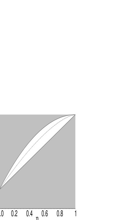
Figure 1:   The narrow constrained physical domain of the function $\rho=\rho_{BRG}^{int}\left(\eta;\!\rho\!_{*}\!,\!\rho_{C}\right)$, defined by its properties i) – vi).          

These general properties entail the representation:

$$\rho_{BRG}^{int}\left(\eta;\!\rho\!_{*}\!,\!\rho_{C}\right)\!=\!\rho_{C}\!+\!(\rho\!_{*}\!-\!\rho_{C})\eta\!+\!(\rho\!_{*}\!-\!\rho_{C})\eta(1\!-\!\eta)q(\eta;\!\rho\!_{*}\!,\!\rho_{C})$$

with some nonnegative function $q(\eta;\rho_{*},\rho_{C})\in[0,1]$, which is bounded and continuous in the 3D domain $\{\eta\in[0,1],\,\rho_{*}\geq\rho_{C}>0\}$.

Actually the function $q(\eta;\rho_{*},\rho_{C})$ is to be find from Eq. (VII.3) and depends on the HG solution of ETOV system with given EOS. As seen in Fig.1, this dependence is quite weak.

Replacing the luminosity variable $\rho$ in corresponding HG-expressions (IV.2) by the function (VII.4), in the interior of the star we obtain the stelar quantities in BRG:

$$m\!=\!m^{BRG}\left(\!{r\over{r_{*}}};\rho_{*},\rho_{C}\!\right)\!,\,m_{0}\!=\!m_{0}^{BRG}\left(\!{r\over{r_{*}}};\rho_{*},\rho_{C}\!\right),$$

$$p\,=\,p^{BRG}\left(\!{r\over{r_{*}}};\rho_{*},\rho_{C}\!\right),\,\,\,\varepsilon=\varepsilon^{BRG}\left(\!{r\over{r_{*}}};\rho_{*},\rho_{C}\!\right)\,,\,\,$$

$$\varphi=\varphi^{BRG}\left(\!{r\over{r_{*}}};\rho_{*},\rho_{C}\!\right);\,\,\,\hbox{-- for}\,\,\,r\in[0,r_{*}].\hskip 39.83368pt$$ (VII.5)

VII.2 The Matching of the BGR Inner and Exterior Solutions

The BRG-solution in the exterior vacuum domain can be obtained making use of Birkhoff theorem in corresponding BRG radial variable $r$. According to F03 it is:

$$\rho_{BRG}^{ext}(r)\!=\!{{2m_{*}}\over{1\!-\!\varrho_{*}^{2}e^{2r/m_{*}}}}\,\,\,\hbox{for}\,\,\,r\!\in\!\big{[}r_{*},m_{*}\ln({1/{\varrho_{*}}})\big{)}.\hskip 17.07182pt$$ (VII.6)

Now we have to match interior and exterior solutions using proper physical requirements on the luminosity variable $\rho$:

1) Because the luminosity of physical source of any kind of radiation is $L=const/4\pi\rho(r)^{2}$, we see that in absence of surface sources of the corresponding radiation the function $\rho(r)$ must be continuous. Otherwise we will destroy the local energy conservation at the place, where $\rho(r)$ has a jump.

2) The jumps of the derivative $\rho^{\prime}(r)$ will induce jumps of the radial derivative of the luminosity, $L^{\prime}(r)$. This means a jumps of the radial derivative of surface energy density. Such phenomenon is physically possible only in presence of some surface agent, like surface force (surface pressure) due to some surface tension. Hence, in this case the star will have some thin crust. Similar phenomenon is familiar, for example, from theory of neutron stars books ; ns , where the crust is introduced and studied from different point of view.

The presence of the crust will obviously yield an observable consequences. Indeed, in this case, according to Eq. (VII.2), the coefficient $\bar{\Gamma}_{r}$ in d’Alembert operator $g^{\mu\nu}\nabla_{\mu}\nabla_{\nu}=g^{\mu\nu}\left(\partial_{\mu}\partial_{\nu}-\bar{\Gamma}_{\mu}\partial_{\nu}\right)$ will be singular at the stelar surface:

$$\bar{\Gamma}_{r}=-\digamma\delta(r-r_{*}).$$ (VII.7)

Here $\delta(r)$ is 1D Dirac delta function. We refer to the quantity $\digamma$ as to ”crust parameter”. Its role in field propagation through the stelar surface will be considered in the next Subsection.

If we exclude the presence of stelar crust and corresponding jump of the radial derivative $L^{\prime}(r)$, the crust parameter will be zero: $\digamma=0$ and the derivative $\rho^{\prime}(r)$ of the luminosity variable will be continuous function

It is obvious that the justification of the matching conditions is impossible without right physical interpretation of the luminosity variable $\rho$.

The above physical considerations entails the following mathematical consequences:

1. The continuity condition $\rho_{BRG}(r_{*}\!-\!0)\!=\!\rho_{BRG}(r_{*}\!+\!0)$ gives the basic relation

$$r_{*}=m_{*}\ln\left({1\over\varrho_{*}}\sqrt{1-{{2m_{*}}\over{\rho_{*}}}}\right)<r_{\infty}.$$ (VII.8)

The finite value $r_{\infty}:=m_{*}\ln(1/\varrho_{*}))$ corresponds to the physical space-infinity in BGR, i.e., to the geometric place of points in 3D space, where the luminosity variable $\rho(r)\to\infty$ for $r\to r_{\infty}-0$ and the 4D spacetime is asymptotically flat.

Hence, as in the case of point particle source of gravity F03 , in BRG we have to consider the finite interval $r\in[0,r_{\infty})$ as a real physical domain of the radial variable $r$. In comparison with the point particle problem, the difference is that in stelar models we have different forms – (VII.4) and (VII.6) of the gauge function $\rho_{BGR}(r)$ in the interior domain of the star and in the exterior vacuum domain.

2. One can easily find that for the exterior solution (VII.6) the value of the constant in Eq. (VII.2) is $const=1/m_{*}^{2}$.

Taking into account that:

a) The quantities $\rho$, $g_{\rho\rho}$ and $g_{tt}$ are continuous functions of the radial variable at the point $r=r_{*}$; and

b) The derivative $\rho_{BRG}^{\prime}(r)>0$ is positive everywhere in the physical domain of the BGR-radial variable $r$;

we can describe the jump of this derivative by the formula

$$\rho_{BRG}^{\prime}(r_{*}\!+\!0)=e^{-\digamma}\rho_{BRG}^{\prime}(r_{*}\!-\!0),\,\,\,\digamma\in(-\infty,\infty).\hskip 17.07182pt$$ (VII.9)

Obviously, for $\digamma\neq 0$ this formula describes a refraction of the lines $\rho=\rho(r)$ at the point $r_{*}$. It yields the relation

$$e^{\digamma}={{m_{*}}^{2}\over{r_{*}}}\int_{\rho_{C}}^{\rho_{*}}{{d\rho}\over{\rho^{2}}}\sqrt{{-g_{\rho\rho}}\over{g_{tt}}}.$$ (VII.10)

Now, making use of the already found HG functions $m_{*}(\rho_{*},\rho_{C})$ and $m_{0}(\rho_{*},\rho_{C})$, and matching conditions (VII.8) and (VII.10), we can solve the algebraic system of four equations

$$m_{*}(\rho_{*},\rho_{C})-m_{*}=0,$$

$$m_{0}(\rho_{*},\rho_{C})-m_{0*}=0,$$

$$\left({{m_{*}}\over{m_{0*}}}\right)^{2}\!\exp\!\left(2{r_{*}}\over{m_{*}}\right)\!+\!{{2m_{*}}\over{\rho_{*}}}-1=0,$$

$${m_{*}}^{2}\int_{\rho_{C}}^{\rho_{*}}{{d\rho}\over{\rho^{2}}}\sqrt{{-g_{\rho\rho}}\over{g_{tt}}}-r_{*}e^{\digamma}=0\,\,\,$$ (VII.11)

for six unknowns $m_{*},m_{0*},\rho_{C},\rho_{*},r_{*},\digamma$ with respect to the first four of them. Thus we arrive at a new form of our solutions for relativistic stelar models with given EOS:

$$m_{*}=m_{*}^{\,BRG}(r_{*},\digamma),\,\,m_{0*}=m_{0*}^{\,BRG}(r_{*},\digamma),$$

$$\rho_{*}=\,\rho_{*}^{\,BRG}(r_{*},\digamma)\,,\,\,\,\,\rho_{C}\,=\,\rho_{C}^{\,BRG}(r_{*},\digamma).\,\,$$ (VII.12)

This representation sheds a new light on the physical meaning of the two-parameter family of relativistic stars, obtained in present article: The constant parameter $\digamma$ defines the properties of stelar crust. For different values of this parameter we obtain relativistic stars with different crusts.

After all, if we fix the value of the parameter $\digamma$, we will obtain one parameter family of relativistic stars, precisely as in Newton theory of stars and in the standard relativistic approach to stelar physics books , but without extra condition $\rho_{C}=0$.

For example, postulating continuity of the derivative $\rho_{BRG}^{\prime}(r)$ at the stelar edge $r=r_{*}$, we obtain $\digamma=0$.

The existence of one parameter family of relativistic stars with arbitrary fixed value of the parameter $\digamma$ becomes possible just for the sake of matching conditions (VII.8) and (VII.10). The condition (VII.10) replaces the HG extra condition $\rho_{C}=0$ and produces a new type of stiff relations in stelar physics.

It is obvious that one can impose only one of these alternative extra conditions. A novel problem in stelar astrophysics is to verify which one of them, if any, takes place in Nature.

VII.3 Spreading of Waves and Static Fields Trough the Stelar Crust

The physical agent, which brings into being the stelar crust, changes the space-time geometry in accord to condition (VII.9). Therefore the presence of the crust will influence the spreading of all possible physical wave fields: scalar, electromagnetic, gravitational, spinor, e.t.c.

In this subsection we will present a preliminary investigation of the spreading of waves and static fields through the stelar crust. Our aim is to reach qualitative understanding of possible role of the stelar crust for field’s dynamics and statics. Therefore we consider in proper approximation only the simplest case of scalar spherically symmetric field $\Phi(t,r)$. To distinguish the effects, caused by the stelar crust, here we neglect the interaction of the wave fields with the stelar matter. The exact treatment of this issue is a complicated problem. Its consideration requires first to have a complete solution for some specific background stelar model.

As a result of Eq. (VII.7) one obtains for field $\Phi(t,r)$ in BRG the following wave equation:

$$g^{\mu\nu}\!\nabla_{\mu}\!\nabla_{\nu}\!\Phi\!=\!g^{tt}\Phi_{tt}\!+\!g^{rr}\Phi_{rr}\!+\!\digamma\delta(r-r_{*})\Phi_{r}\!=\!0.\,\,\,$$ (VII.13)

Owing to the continuity of functions $g^{tt}(r)$ and $g^{rr}(r)$ at point $r_{*}$, we can replace them in a small enough vicinity of the crust with their constant values $g^{tt}(r_{*})$ and $g^{rr}(r_{*})$. Then, changing the corresponding scales of time and radial variables : $t\rightarrow\sqrt{g_{tt}(r_{*})}\,t$ and $r\rightarrow\sqrt{g_{rr}(r_{*})}\,r$, and using the properties of Dirac $\delta$-function, we arrive at the differential equation:

$$\Phi_{tt}\!-\!\Phi_{rr}\!+\!\digamma\delta(r-r_{*})\Phi_{r*}=0,$$ (VII.14)

where $\Phi_{r*}=\Phi_{r}(t,r_{*})$ is the value of the first derivative $\Phi_{r}(t,r)$ at the stelar edge.

The general solution of this equation can be represented in the form of Fourier integral:

$$\Phi(t,r)=\int_{-\infty}^{\infty}d\omega e^{i\omega t}R(r;r_{*},\omega).$$ (VII.15)

The amplitudes $R(r;r_{*},\omega)$ are described by the general solution

$$R(r;r_{*},\omega)=R(r_{*},\omega)\cos\big{(}\omega(r-r_{*})\big{)}+\hskip 45.52458pt$$

$$R_{r}(r_{*},\omega)\Big{(}1+\digamma\Delta\Theta\big{(}\omega(r-r_{*})\big{)}\Big{)}{{\sin\big{(}\omega(r-r_{*})\big{)}}\over\omega}\hskip 28.45274pt$$ (VII.16)

of the second order ordinary differential equation:

$$R_{rr}\!+\omega^{2}R\!=\!\digamma\delta(r-r_{*})R_{r}(r_{*},\omega).$$ (VII.17)

Here the arbitrary functions $R(r_{*},\omega)=R(r_{*};r_{*},\omega)$ and $R_{r}(r_{*},\omega)=R_{r}(r_{*};r_{*},\omega)$ appear as integration constants of Eq. (VII.17) and for corresponding values of $\omega$ present the values of the function $R(r;r_{*},\omega)$ and its first derivative $R_{r}(r;r_{*},\omega)$ at the edge of the star; $\Theta(x)$ is the Heaviside step function. For our purposes we have to regularize this generalized function Gelfand , i.e., we have to prescribe some definite value $\Theta(0)$ to this function at the point $x=0$. Then $\Delta\Theta(x):=\Theta(x)-\Theta(0)$.

Now it becomes clear that:

1. The physical role of the stelar crust is to produce a jump in the $\sin$-mode of the stationary waves (VII.16). At the same time the $\cos$-mode remains unchanged, crossing the crust.

2. If $\digamma=0$, i.e., in absence of stelar crust, both modes spread trough the edge of the star as a completely free waves.

3. Choosing $R(r_{*},\omega)=0$ and proper special values of $\Theta(0)$, one can obtain solutions, which describe stationary waves only inside the star:

$$R^{ins}(r;r_{*},\omega)\!=-\digamma R_{r}(r_{*},\omega)\Theta\big{(}-\omega(r\!-\!r_{*})\big{)}{{\sin\big{(}\omega(r\!-\!r_{*})\big{)}}\over\omega},$$

– for $\Theta(0)=1+1/\digamma$, or only outside the star:

$$R^{outs}(r;r_{*},\omega)\!=\!\digamma R_{r}(r_{*},\omega)\Theta\big{(}\omega(r\!-\!r_{*})\big{)}{{\sin\big{(}\omega(r\!-\!r_{*})\big{)}}\over\omega}$$

– for $\Theta(0)=1/\digamma$.

Thus we see that the parameter $\Theta(0)$ plays the role of reflection coefficient for the $\sin$-mode. For proper values of this coefficient we have a total inner, or total outer reflection of the $\sin$-mode by the stelar crust.

4. In the static limit $\omega\to 0$ one obtains from Eq. (VII.16):

$$\Phi(r)\!=\!\Phi(r_{*})\!+\!\Phi_{r}(r_{*})\big{(}1\!+\!\digamma\Delta\Theta(r\!-\!r_{*})\big{)}(r\!-\!r_{*}).\hskip 14.22636pt$$ (VII.18)

The last formula shows that crossing the stelar crust with $\digamma\neq 0$, the static field $\Phi(r)$ is a subject of refraction.

The existence of the stelar crust with the above properties is a new specific prediction of our models of relativistic stars. It may have important consequences not only for the stelar physics and needs further careful study.

VIII The Solution of the ETOV System in Physical Regular Gauge

The regular change of the rho-gauge, defined by the fractional linear mapping of the interval $r\in[0,r_{\infty})$ onto the whole interval $r\in[0,\infty)$:

$$r\to m_{*}\ln(1/\varrho_{*}){{r}\over{r+m_{*}/\ln(1/\varrho_{*})}}$$ (VIII.1)

brings us to the physical regular gauge (PRG) F03 . There the radial variable $r$ varies in the standard semi-infinite interval $[0,r_{\infty})$. (Note that we are using the same notations $r,\,r_{*},...$ for radial variables in different $\rho$-gauges.) Then in PRG we have

$$\rho_{PRG}(r)=\begin{cases}\rho_{BRG}^{int}\left(\eta;\rho_{*},\rho_{C}\right)\,\,\,\,,&\text{if $r\in[0,r_{*}]$};\\ 2m_{*}\left(1-e^{2\varphi_{G}}\right)^{-1},&\text{if $r\in[r_{*},\infty),$}\end{cases}\hskip 17.07182pt$$ (VIII.2)

where now

$$\eta={{r(r_{*}+m_{*}/\ln(1/\varrho_{*}))}\over{r_{*}(r+m_{*}/\ln(1/\varrho_{*}))}}\in[0,1]\,\,\,\hbox{for}\,\,\,r\in[0,r_{*}],\hskip 17.07182pt$$ (VIII.3)

$$r_{*}\!=\!m_{*}\left(\!{1/{\ln\left({1}\over{\sqrt{1\!-\!{{2m_{*}}\over{\rho_{*}}}}}\right)}}\!-\!1/\ln\left({1\over\varrho_{*}}\right)\!\right)\geq 0.\hskip 17.07182pt$$ (VIII.4)

In Eq. (VIII.2) we are using the modified Newton gravitational potential F03 :

$$\varphi_{\!{}_{G}}(r;m_{*},m_{0*}):=-{{m_{*}}\over{r+m_{*}}/\ln({m_{0*}\over m_{*}})}.$$ (VIII.5)

From Eq. (VIII.2) one easily obtains the important inequality for the stelar parameters, written in the following two useful forms:

$$f_{*}:=\varrho_{*}^{2}+{{2m_{*}}\over{\rho_{*}}}\leq 1\,\,\,\Leftrightarrow\,\,\,\rho_{*}\geq{{2m_{*}}\over{1-\varrho_{*}^{2}}}.$$ (VIII.6)

This is a more strong restriction on the domain $\mathbb{D}^{(2)}_{\rho_{*},\rho_{C}}$ than the inequality (V.9b). Actually the inequality (VIII.6) is a direct consequence of matching condition $\rho(r_{*}-0)=\rho(r_{*}+0)$, written in the following BRG-form:

$$1=\varrho_{*}^{2}e^{2{r_{*}}\over{m_{*}}}+{{2m_{*}}\over{\rho_{*}}}\Rightarrow 1\geq\varrho_{*}^{2}+{{2m_{*}}\over{\rho_{*}}}\,\,\,\hbox{for}\,\,\,r_{*}\geq 0.$$

IX Some Concluding Remarks

It is clear that the new approach to stelar structure, developed in the present article, calls for revision of many of widely accepted features of the GR theory of stars. The changes are not based on the critics of the very GR, but on more deep understanding of its applications, and on solution of some open problems in this theory, like the physical justification of the choice of GR gauges.

In particular, it is obvious that we must apply the Birkhoff theorem in PRG only in the interval $\rho\in[\rho_{*},\infty)\rightleftarrows r\in[r_{*},\infty)$, i.e. in the exterior vacuum domain outside the star. As a result, in this domain all local GR effects like gravitational redshift, perihelion shift, deflection of light rays, time-delay of signals, etc., are gauge invariant and will have their standard exact values. The PRG metric for this domain can be found in F03 . The differences between predictions of our general models of stars and the standard ones, based on the assumption $\rho_{C}=0$, can not be observed in the local gauge invariant gravitational phenomena, which take place in the outer vacuum domain, surrounding the stars.

Hence, our most general geometrical models have an essential impact only on the theory of the interior of relativistic stars, and on theory of spreading of different physical fields in stars, and around the stars.

The obtained new results seems to deserve further study and can lead to serious changes of our understanding of physics of stars in Nature. Specific models of the described novel type for relativistic stars with different EOS, as well as other developments and applications to problems of real stelar physics, will be published in subsequent articles of this series.

Acknowledgments

The author is grateful to the High Energy Physics Division, ICTP, Trieste, for the hospitality and for the nice working conditions during his visit in the autumn of 2003. There an essential basic ideas of present article were developed.

The author is vary grateful, too, to the JINR, Dubna, for the financial support of the present article and for the hospitality and good working conditions during his two three-months visits in 2003 and in 2004, when the most of the work has been done.

The author is deeply indebted to Prof. T. L. Boyadjiev for friendly support and many useful discussions on mathematical problems, related to the stelar boundary problem, to Prof. S. Bonazzola, for discussions, and especially, for encouraging general information about the existence of results in direction of overcoming of the standard relativistic restriction on the stelar masses. Similar results can be found in the articles Bell , too. The author wishes to thank Prof. Ll. Bell for attracting his attention to these articles.

The author is tankful, too, to Prof. V. Nesterenko and to unknown referee of the first of the articles F03 , who raised the problem of point particle limit of bodies of finite dimension in GR, thus stimulating the development of general geometrical models of relativistic stars.

References

- (1) L. D. Landau, E. M. Lifshitz, The Classical Theory of Fields, 2d ed.; Reading, Mass: Addison-Wesley, 1962; V. A. Fock, The Theory of Space, Time and Gravitation, Pergamon, Oxford, 1964. B. K. Harrison, K. S. Thorne, M. Wakano, J. A. Wheeler, Gravitational Theory and Gravitational Collapse, University of Chikago Press, 1965. R. C. Tolman, Reativity, Thermodynamics and Cosmology, Claderon Press, Oxford, 1969. S. Weinberg, Gravitation and Cosmology, Wiley, N.Y., 1972; C. Misner, K. S. Thorne, J. A. Wheeler, Gravity, W. H. Freemand & Co., 1973. R. Adler, M. Bazin, M. Schiffer, Introduction to General Relativity, McGraw-Hill Book Comp., 1965. D. Kramer, H. Stephani, M. Maccallum, E. Herlt, Ed. E. Schmutzer, Exact Solutions of the Einstein Equations, Deutscher Verlag der Wissenschaften, Berlin, 1980. S. L. Shapiro, S. A. Teukolsky, Black Holes, White Dwarfs and Neutron Stars, Jhon Wiley & Sons, 1985. H. Stephani, General Relativity. An introduction to the theory of the gravitational field, 2nd edition, Cambridge University Press, 1990. G. S. Saakjan, The Physics of Neutron Stars, 2nd eddition, Ereven University Press, 1988. H. Stephani, D. Kramer, M. Maccallum, E. Herlt, Exact Solutions of Einstein’s Field Equations, 2nd eddition, Cambridge University Press, 2003.
- (2) S. Chandrasekhar, Ap. J. 74, 81 (1931); MNRAS, 95, 207 (1935). L. Landau, Physik Zeits. Sowiet Union 1, 285 (1932).
- (3) S. Chandrasekhar, MNRAS 93, 390 (1933). T. Hamada, E. E. Salpeter, ApJ 134, 683 (1961). M. A. Wood, in Proc. 9th European Workshop on White Dwarfs, ed. D. Koester, K. Werner, Springer, 41, 1990.
- (4) Schwarzschild K., Sitz. Preuss. Acad. Wiss., 424 (1916).
- (5) R. Tolmen, Phys. Rev. 55, 364 (1939). Openheimer J. R., Volkoff G. M., Phys. Rev. 55, 374 (1939).
- (6) H. Bondi,Proc, Roy. Soc. (London), A 281, 39 (1964). H. Bondi, Mon. Not. Roy. Astr. Soc. 107, 410 (1947). H. A. Buchdahl, Phys. Rev. 116, 1027 (1959). J. B. Hartle, Phys. Rep. 46, 202 (1978). G. F. R. Ellis, R. Maartens, S. D. Neil, M. N. R. A. S.184, 439 (1978). C. B. Collins, J. Math. Phys. 26, 2268 (1985).
- (7) A. Broderick, M. Prakash, J. M. Lattimer, The Equation of State of Neutron-Star Matter in Strong magnetic Fields, astro-ph/0001537. J. M. Lattimer, M. Prakash, Nuclear Matter and its Role in Supernovae, Neutron Stars and Compact Objects Binary Mergers, astro-ph/0002203; Neutron Star Structure and the Equation of State, astro-ph/0002232. H. Heiselberg, Neutron Star Masses, Radii and Equation of State, astro-ph/0201465. P. Haensel, Equation of State of Dense Matter and Maximum Mass of Neutron Stars, astro-ph/0301073. I. A. Morrison, T. W. Baumgarte, S. L. Shapiro, Effect of Differential Rotation on the Maximum Mass of Neutron Stars: Relativistic Nuclear Equations of State, astro-ph/0401581. E. Weber, Strange Quark Matter and Compact Stars, astro-ph/0407155.
- (8) W. Becker, G. Pavlov, Pulsars and Isolated Neutron Stars, astro-ph/0208356. J. M. Lattimer, M. Prakash, The Physics of Neutron Stars, astro-ph/0405263.
- (9) L. S. Finn, Observational Constraints on the Neutron Star Mass Distribution, astro-ph/9409053. B. Link, R. I. Epstein, Pulsar Constrains on Neutron Star Structure and Equation of State, astro-ph/9909146; Probing Neutron Star Interior with Glitches, astro-ph/0001245. J. A. Pons, F. M. Walter, J. M. Lattimer, M. Prakash, R. Neuhäuser, P. An, Tawards a Mass and Radius Determination of the Nearby Isolated neutron Star RX J185635-3754, astro-ph/0107404. F. Walter, J. Lattier, A Revised Parallax and its Implications for J185635-3754, astro-ph/0204199. D. Gondek-Rosiśka, W. Kluźniak, N. Stergioulas, An Unusual Low Mass for Some ”Neutron” Stars ?, astro-ph/0206470. T. M. Braje, R. W. Romani, RX J185635-3754: Evidence for a Stiff EOS, astro-ph/0208069. M. Prakash, J. M. Lattimer, Observability of Neutron Stars with Quarks, astro-ph/0209122; A Tile of Two Mergers: Searching for Strangeness in Compact Stars, astro-ph/0305306. D. J. Nice, E. M. Splaver, Heavy Neutron Stars? A Status Report on Acrecibo Timming of Four Pulsar-White Dwarf Systems, astro-ph/0311296. J. E. Trümper, V. Burwitz, F. Haberl, V. E. Zavlin, The Puzzles of RX J185635-3754, astro-ph/0312600.
- (10) J. L. Grenstein, J. B. Oke, H. L. Shipman, ApJ, 169, 563 (1971). H. L. Shipman, ApJ, 177, 723 (1972). H. L. Shipman, ApJ, 213, 138 (1977). H. L. Shipman, ApJ, 228, 240 (1979). H. L. Shipman, C. A. Saas, ApJ., 235, 177 (1980). S. Vennes, J. R. Thorstensen, P. Thejll, H. L. Shipman, ApJ, 372, L37 (1991). J. L. Provencal, H. L. Shipman, E. Hg, P. Thejll, ApJ, 494, 759 (1998). J. A. Panel, L. G. Althaus, O. G. Benvenuto, Astron. Astrophys., 353, 970 (2000). J. Madej, M. Naleźyty, L. G. Althaus, Mass Distribution of DA White Dwarfs in the First Data Release of Sloan Digital Sku Survey, astro-ph/0404344.
- (11) A. Celotti, J. C. Miller, D. W. Sciama, Astrophysical Evidence for Existence of Black Holes, astro-ph/9912186. V. P. Frolov, I. D. Novikov, Black Hole Physics, Kluwer Acad. Publ., 1998. M. A. Abramowicz, W. Kluźniak, J-P. Lasota, Astron. Astrophys., 396, L31 (2002); astro-ph/0207270. R. Narayan, Evedences for the Black Hole Event Horison, astro-ph/0310692. S. L. Robertson, D. J. Leiter, On the Origin of the Universal Radio-X-Ray Luminosity Correlation in Black Hole Candidates, astro-ph/0405445. R. Fender et all, Nature, 427, p.222 (2004).
- (12) P. Fiziev, Gravitational Field of Massive Point Particle in General Relativity, gr-qc/0306088, ICTP preprint IC/2003/122. P.P. Fiziev, T.L. Bojadjiev, D.A. Georgieva, Novel Properties of Bound States of Klein-Gordon Equation in Gravitational Field of Massive Point, gr-qc/0406036. P. Fiziev, S. Dimitrov, Point Electric Charge in General Relativity, hep-th/0406077. P. Fiziev, On the Solutions of Einstein Equations with Massive Point Source, gr-qc/0407088.
- (13) A. S. Eddington, The mathematical theory of relativity, 2nd ed. Cambridge, University Press, 1930 (repr.1963).
- (14) K. Schwarzschild, Sitzungsber. Preus. Acad. Wiss. Phys. Math. Kl., 189 (1916).
- (15) M. Brillouin, Le Journal de physique et Le Radium 23, 43 (1923).
- (16) P. A. M.Dirac, Proc. Roy Soc. (London), A270, 354 (1962); Conference in Warszawa and Jablonna, L. Infeld ed., Gauthier-Villars, Paris (1964), pp. 163-175.
-
(17)
http://www.rundetaarn.dk/engelsk/observatorium/ hrd1.html
;
http://images.gsfc.nasa.gov/docs/teachers/lifecycles/ Image31.gif . - (18) J. N. Bahcall, M. H. Pinsonneault, Rev. Mod. Phys. 67, 781 (1995); J. N. Bahcall, Nucl. Phys. B (Proc. Suppl.) 77, 64 (1999); J. N. Bahcall, M. H. Pinsonneault, Sabrani Basu, Astrophys. J. bf 555, 990 (2001); J. N. Bahcall, C. Pea-Garay, New J. Phys. 6, 63 (2004).
- (19) R. F. Tooper, ApJ, 140, 434 (1964). S. A. Bludman, ApJ, 183, 637 (1973). S. C. Pandey, M. C. Dugapal, A. K. Pande, Astrophys. and Space Sci., 180, 75 (1991).
- (20) L. Schwartz, Théorie des distributions I, II, Paris, 1950-51; I. M. Gel’fand, G. E. Shilov, Generalized Finctions, N.Y., Academic Press, 1964; H. Bremermann, Distrinutions, Complex Variables and Fourier Transform, Addison-Wesley Publ. Co. Reading, Massachusetts, 1965.
- (21) J. M. Aguirregabiria, Ll. Bel, J. Martin, A. Molina, E. Ruiz gr-qc/0104019, Gen. Rel. and Grav. 33 1809 (2001); J. M. Aguirregabiria, Ll. Bel, gr-qc/0105043, Gen. Rel. and Grav. 33, 2049 (2001) ; Ll. Bel, gr-qc/0210057.